
Simulating an Autonomously Operating Low-Cost Static Terrestrial LiDAR for Multitemporal Maize Crop Height Measurements


Abstract
:
1. Introduction
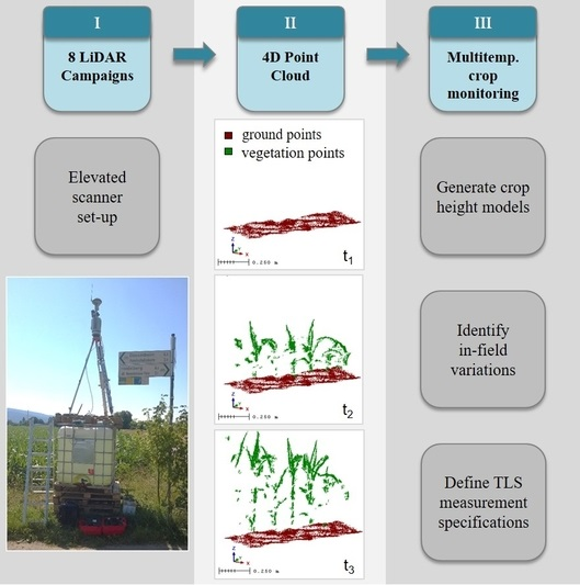
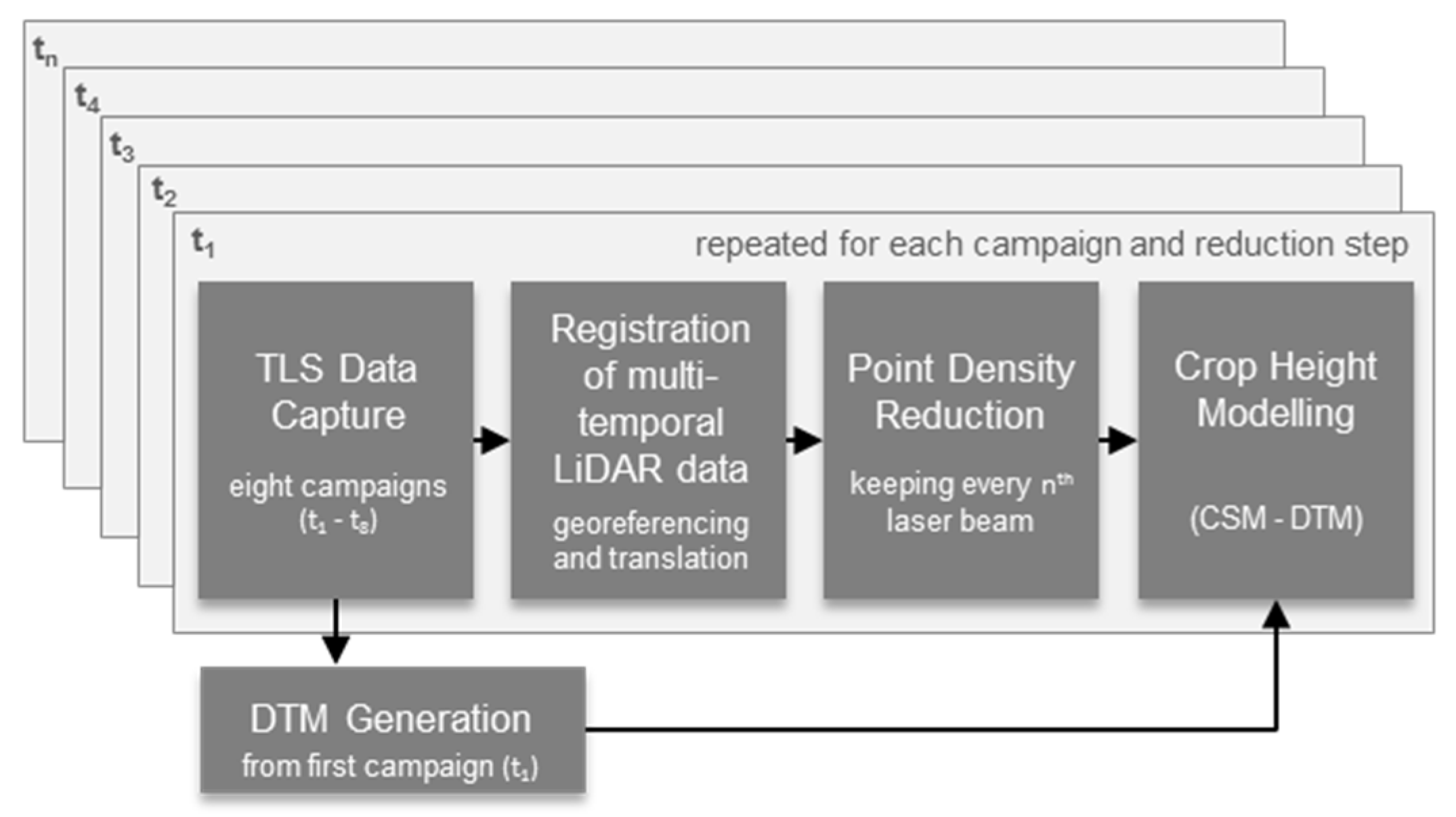
2. Materials and Methods
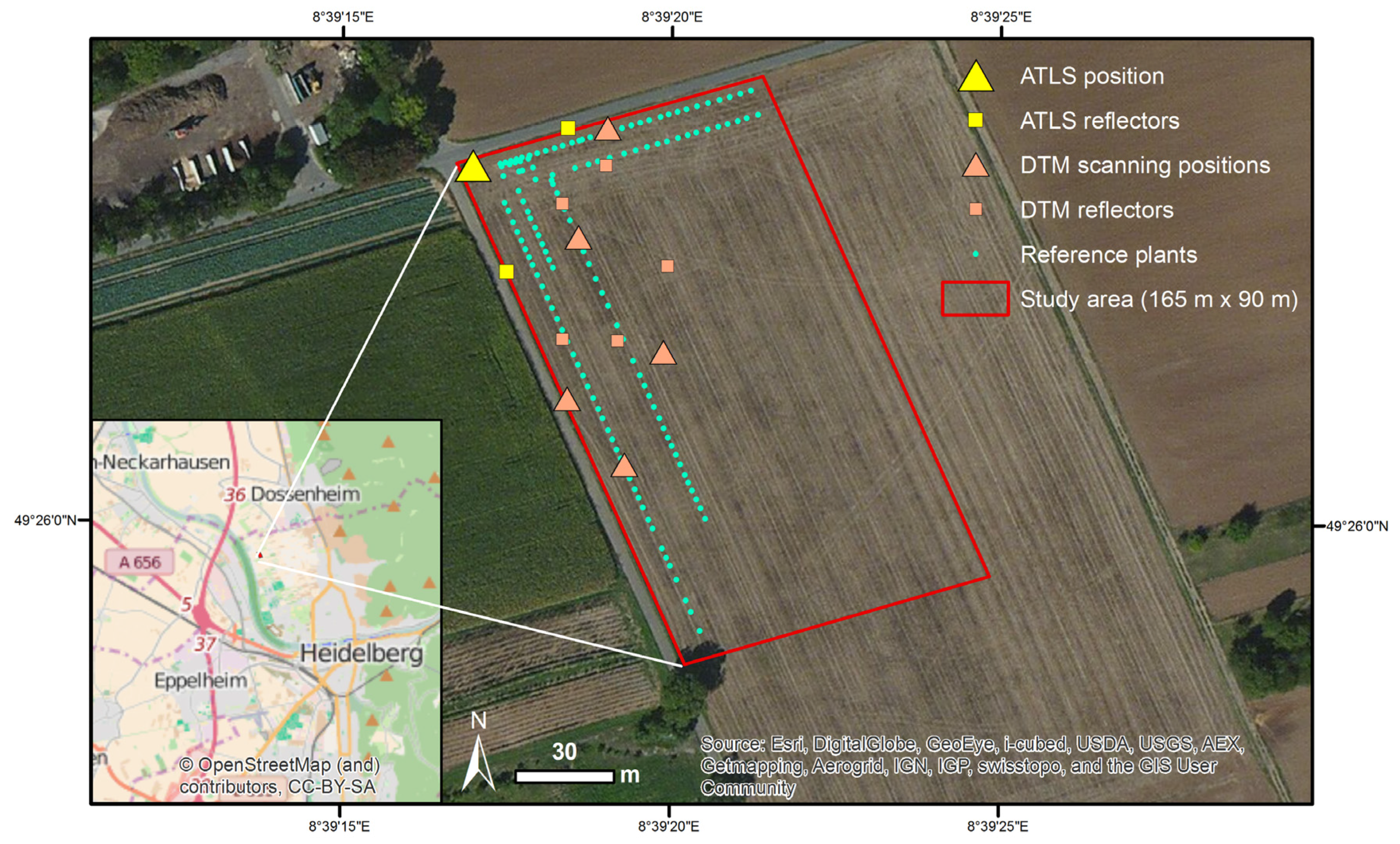
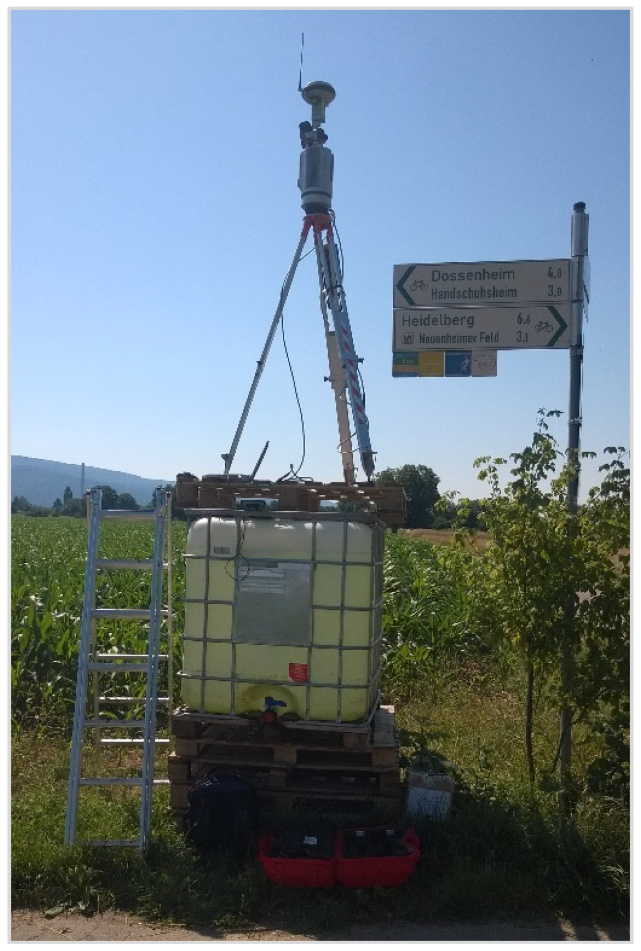
2.1. Study Area and Measurement Set-Up
2.2. Generation of Crop Height Models
2.2.1. DTM Generation
2.2.2. Registering Multitemporal TLS Data
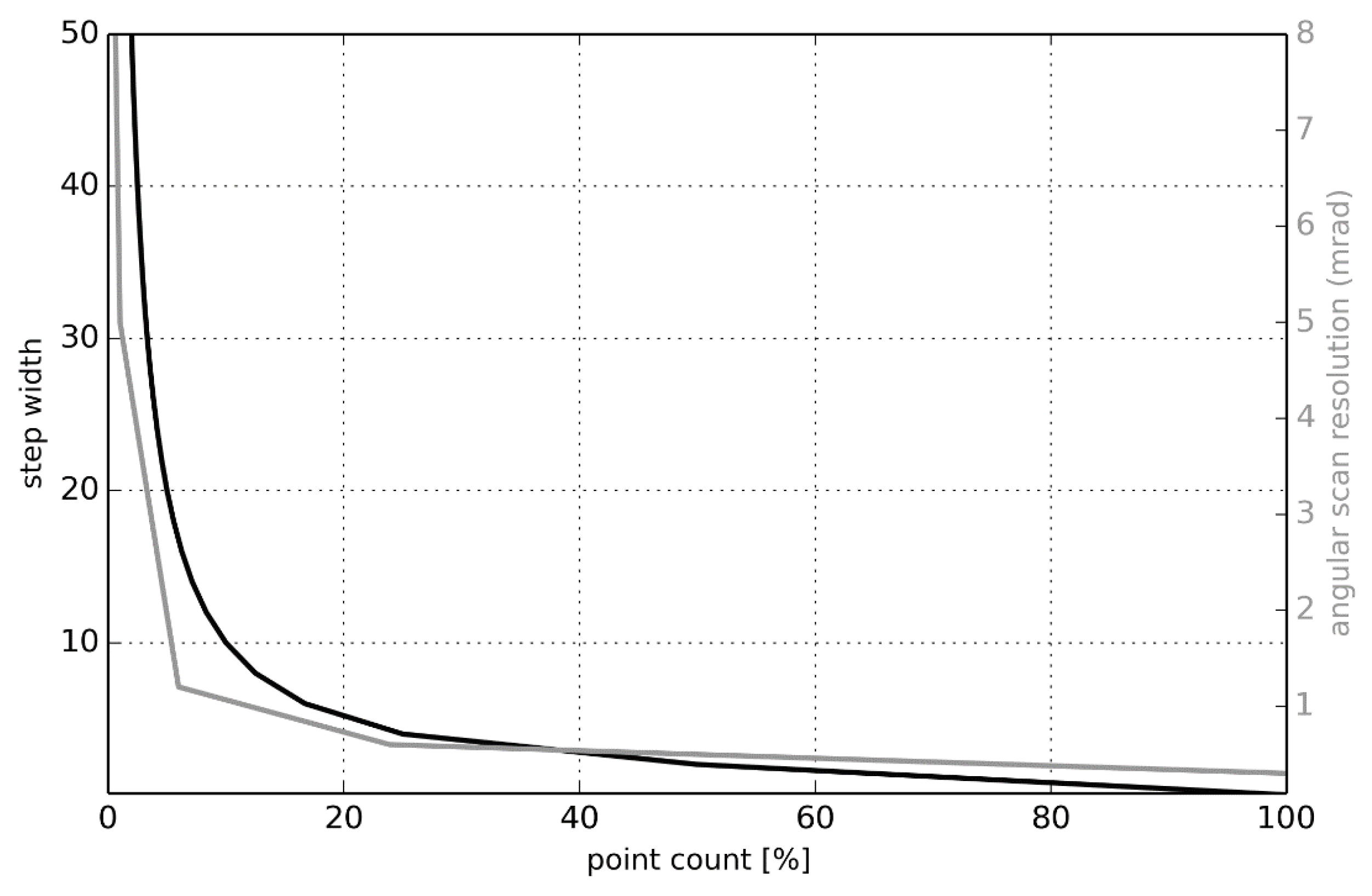
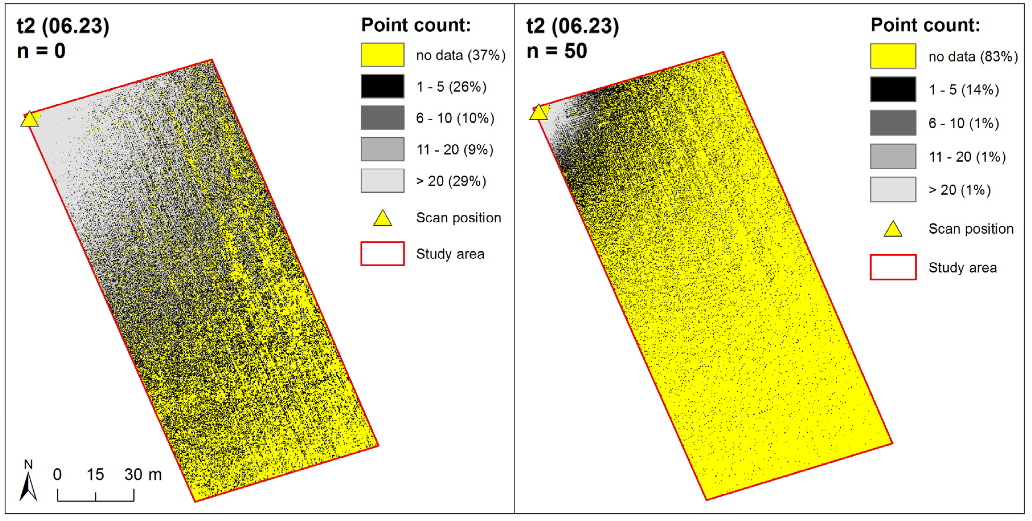
2.2.3. Point Density Reduction
2.2.4. Crop Height Modeling
2.3. Accuracy Assessment of Crop Height Models
2.3.1. Point Density Effects
2.3.2. Distance to Scanner Effects
3. Results
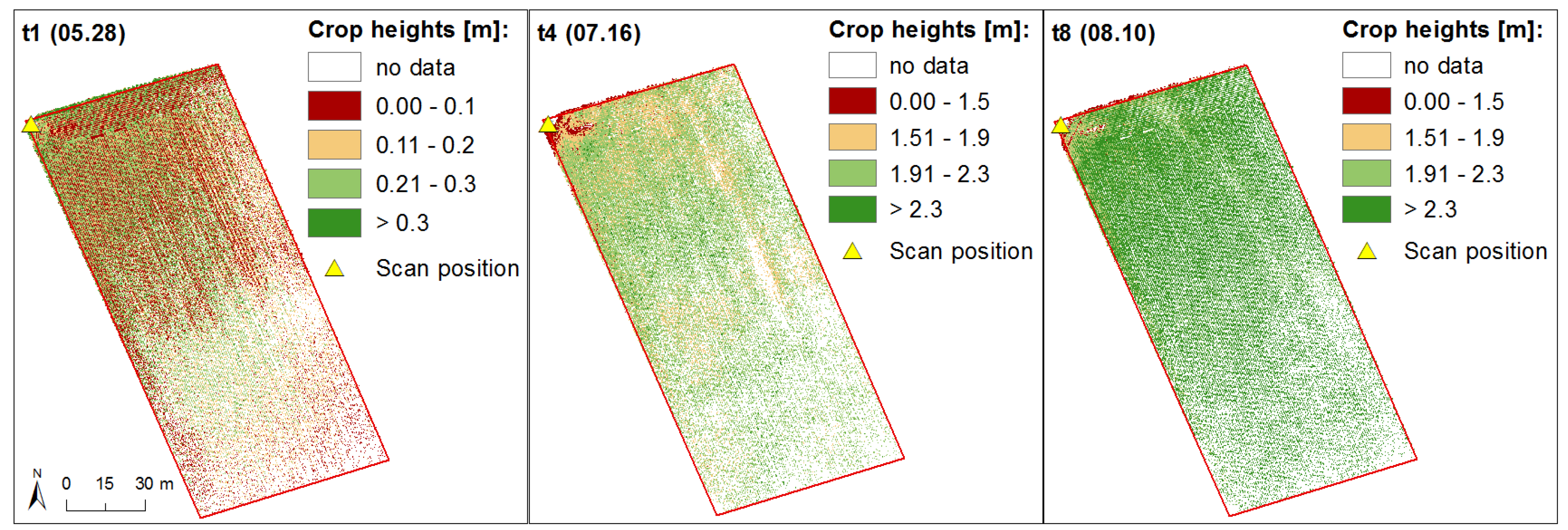
3.1. Generation of Crop Height Models
3.2. Accuracy Assessment of Crop Height Models
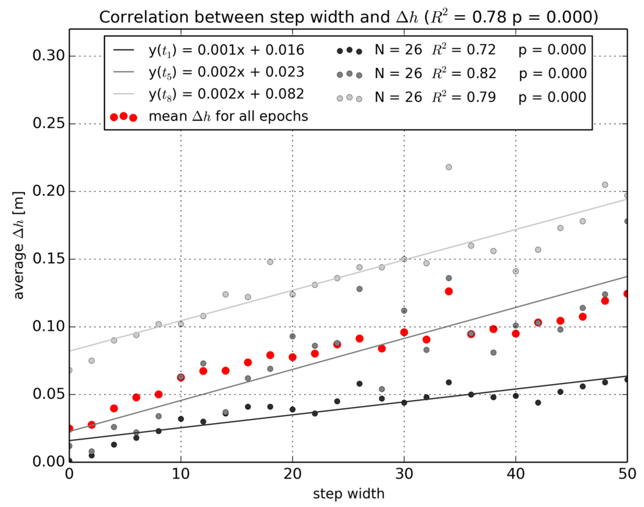
3.2.1. Point Density Effects
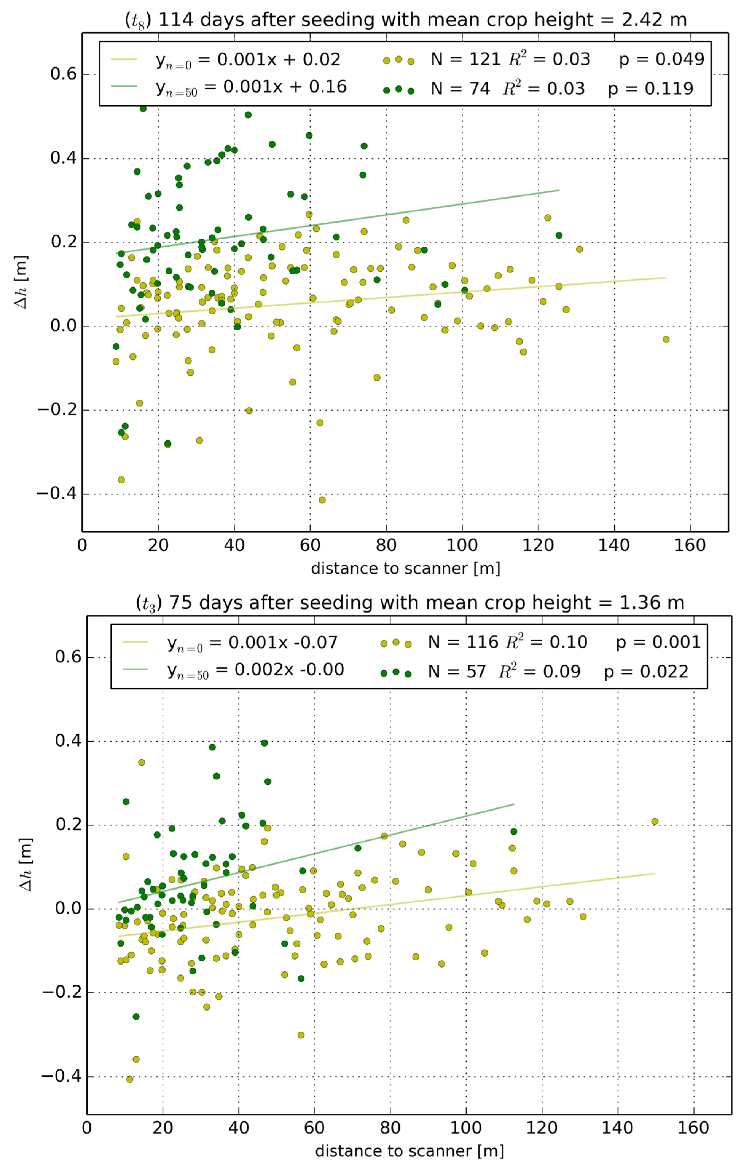
3.2.2. Distance to Scanner Effects
4. Discussion
4.1. Study Area and Measurement Set-Up
4.2. Generation of Crop Height Models
4.3. Accuracy Assessment of Crop Height Models
5. Conclusions and Outlook
Acknowledgments
Author Contributions
Conflicts of Interest
Appendix

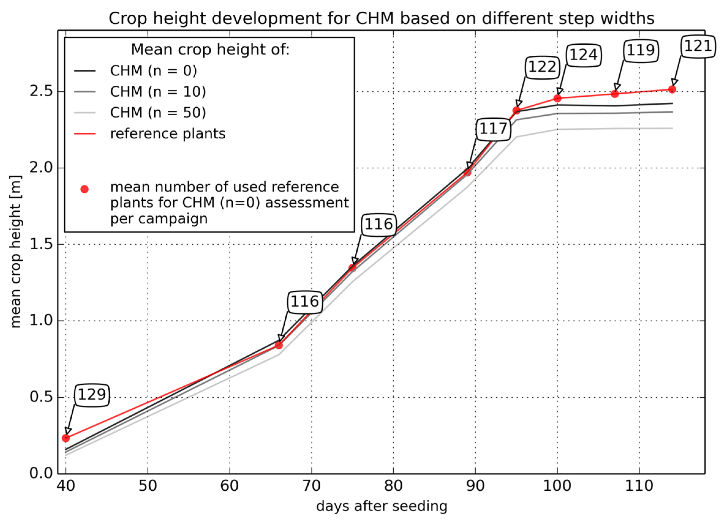
| Campaign (t) | Step Width (n) | Reference Plants Used (N) | Mean Δh (m) | Median Δh (m) | RMSE of Δh (m) |
|---|---|---|---|---|---|
| 1 | 0 | 129 | 0.006 | 0.001 | 0.052 |
| 10 | 102 | 0.035 | 0.032 | 0.065 | |
| 50 | 69 | 0.07 | 0.061 | 0.092 | |
| 2 | 0 | 116 | −0.03 | −0.027 | 0.084 |
| 10 | 99 | 0.006 | 0.007 | 0.103 | |
| 50 | 62 | 0.07 | 0.044 | 0.146 | |
| 3 | 0 | 116 | −0.02 | −0.013 | 0.112 |
| 10 | 98 | 0.025 | 0.026 | 0.118 | |
| 50 | 57 | 0.063 | 0.043 | 0.144 | |
| 4 | 0 | 117 | −0.023 | 0.019 | 0.227 |
| 10 | 91 | 0.005 | 0.038 | 0.218 | |
| 50 | 68 | 0.080 | 0.094 | 0.238 | |
| 5 | 0 | 122 | −0.010 | 0.012 | 0.292 |
| 10 | 91 | 0.027 | 0.063 | 0.289 | |
| 50 | 63 | 0.136 | 0.178 | 0.347 | |
| 6 | 0 | 124 | 0.024 | 0.067 | 0.195 |
| 10 | 99 | 0.068 | 0.12 | 0.216 | |
| 50 | 65 | 0.126 | 0.172 | 0.269 | |
| 7 | 0 | 119 | 0.040 | 0.072 | 0.16 |
| 10 | 103 | 0.098 | 0.113 | 0.204 | |
| 50 | 71 | 0.177 | 0.207 | 0.277 | |
| 8 | 0 | 121 | 0.053 | 0.068 | 0.132 |
| 10 | 100 | 0.097 | 0.102 | 0.163 | |
| 50 | 74 | 0.211 | 0.197 | 0.271 |
References
- Lee, W.S.; Alchanatis, V.; Yang, C.; Hirafuji, M.; Moshou, D.; Li, C. Sensing technologies for precision specialty crop production. Comput. Electron. Agric. 2010, 74, 2–33. [Google Scholar] [CrossRef]
- Rosell, J.R.; Llorens, J.; Sanz, R.; Arnó, J.; Ribes-Dasi, M.; Masip, J.; Escolà, A.; Camp, F.; Solanelles, F.; Gràcia, F.; et al. Obtaining the three-dimensional structure of tree orchards from remote 2D terrestrial LiDAR scanning. Agric. For. Meteorol. 2009, 149, 1505–1515. [Google Scholar] [CrossRef]
- Zhang, N.; Wang, M.; Wang, N. Precision agriculture—A worldwide overview. Comput. Electron. Agric. 2002, 36, 113–132. [Google Scholar] [CrossRef]
- Hämmerle, M.; Höfle, B. Effects of reduced terrestrial lidar point density on high-resolution grain crop surface models in precision agriculture. Sensors 2014, 14, 24212–24230. [Google Scholar] [CrossRef] [PubMed]
- Schellberg, J.; Hill, M.J.; Gerhards, R.; Rothmund, M.; Braun, M. Precision agriculture on grassland: Applications, perspectives and constraints. Eur. J. Agron. 2008, 29, 59–71. [Google Scholar] [CrossRef]
- McCarthy, C.L.; Hancock, N.H.; Raine, S.R. Applied machine vision of plants: A review with implications for field deployment in automated farming operations. Intell. Serv. Robot. 2010, 3, 209–217. [Google Scholar] [CrossRef] [Green Version]
- Giles, D.; Delwiche, M.; Dodd, R. Electronic measurement of tree canopy volume. Trans. ASAE 1988, 31, 264–272. [Google Scholar]
- Zaman, Q.; Salyani, M. Effects of foliage density and ground speed on ultrasonic measurement of citrus tree volume. Appl. Eng. Agric. 2004, 20, 173–178. [Google Scholar] [CrossRef]
- Schumann, A.W. Performance of an ultrasonic tree volume measurement system in commercial citrus groves. Precis. Agric. 2005, 6, 467–480. [Google Scholar]
- Solanelles, F.; Escolà, A.; Planas, S.; Rosell, J.; Camp, F.; Gràcia, F. An electronic control system for pesticide application proportional to the canopy width of tree crops. Biosyst. Eng. 2006, 95, 473–481. [Google Scholar] [CrossRef]
- Llorens, J.; Gil, E.; Llop, J. Ultrasonic and LiDAR sensors for electronic canopy characterization in vineyards: Advances to improve pesticide application methods. Sensors 2011, 11, 2177–2194. [Google Scholar] [CrossRef] [PubMed]
- Phattaralerphong, J.; Sinoquet, H. A method for 3D reconstruction of tree crown volume from photographs: Assessment with 3D-digitized plants. Tree Physiol. 2005, 25, 1229–1242. [Google Scholar] [CrossRef] [PubMed]
- Leblanc, S.G.; Chen, J.M.; Fernandes, R.; Deering, D.W.; Conley, A. Methodology comparison for canopy structure parameters extraction from digital hemispherical photography in boreal forests. Agric. For. Meteorol. 2005, 129, 187–207. [Google Scholar] [CrossRef]
- Bendig, J.; Bolten, A.; Bennertz, S.; Broscheit, J.; Eichfuss, S.; Bareth, G. Estimating biomass of barley using crop surface models (CSMs) derived from UAV-based rgb imaging. Remote Sens. 2014, 6, 10395–10412. [Google Scholar] [CrossRef]
- Andersen, H.J.; Reng, L.; Kirk, K. Geometric plant properties by relaxed stereo vision using simulated annealing. Comput. Electron. Agric. 2005, 49, 219–232. [Google Scholar] [CrossRef]
- Kise, M.; Zhang, Q. Development of a stereovision sensing system for 3D crop row structure mapping and tractor guidance. Biosyst. Eng. 2008, 101, 191–198. [Google Scholar] [CrossRef]
- Rovira-Más, F.; Zhang, Q.; Reid, J. Creation of three-dimensional crop maps based on aerial stereoimages. Biosyst. Eng. 2005, 90, 251–259. [Google Scholar] [CrossRef]
- Bendig, J.; Bolten, A.; Bareth, G. Uav-based imaging for multi-temporal, very high resolution crop surface models to monitor crop growth variability. Photogramm. Fernerkund. Geoinfor. 2013, 2013, 551–562. [Google Scholar] [CrossRef]
- Giuliani, R.; Magnanini, E.; Fragassa, C.; Nerozzi, F. Ground monitoring the light-shadow windows of a tree canopy to yield canopy light interception and morphological traits. Plant Cell Environ. 2000, 23, 783–796. [Google Scholar] [CrossRef]
- Bongers, F. Methods to assess tropical rain forest canopy structure: An overview. Plant Ecol. 2001, 153, 263–277. [Google Scholar] [CrossRef]
- Mulla, D.J. Twenty five years of remote sensing in precision agriculture: Key advances and remaining knowledge gaps. Biosyst. Eng. 2013, 114, 358–371. [Google Scholar] [CrossRef]
- Stuppy, W.H.; Maisano, J.A.; Colbert, M.W.; Rudall, P.J.; Rowe, T.B. Three-dimensional analysis of plant structure using high-resolution X-ray computed tomography. Trends Plant Sci. 2003, 8, 2–6. [Google Scholar] [CrossRef]
- Van der Zande, D.; Hoet, W.; Jonckheere, I.; van Aardt, J.; Coppin, P. Influence of measurement set-up of ground-based LiDAR for derivation of tree structure. Agric. For. Meteorol. 2006, 141, 147–160. [Google Scholar] [CrossRef]
- Paulus, S.; Dupuis, J.; Riedel, S.; Kuhlmann, H. Automated analysis of barley organs using 3D laser scanning: An approach for high throughput phenotyping. Sensors 2014, 14, 12670–12686. [Google Scholar] [CrossRef] [PubMed]
- Van der Heijden, G.; Song, Y.; Horgan, G.; Polder, G.; Dieleman, A.; Bink, M.; Palloix, A.; van Eeuwijk, F.; Glasbey, C. Spicy: Towards automated phenotyping of large pepper plants in the greenhouse. Funct. Plant Biol. 2012, 39, 870–877. [Google Scholar] [CrossRef]
- König, K.; Höfle, B.; Hämmerle, M.; Jarmer, T.; Siegmann, B.; Lilienthal, H. Comparative classification analysis of post-harvest growth detection from terrestrial LiDAR point clouds in precision agriculture. ISPRS J. Photogramm. Remote Sens. 2015, 104, 112–125. [Google Scholar] [CrossRef]
- Watt, P.J.; Donoghue, D.N.M. Measuring forest structure with terrestrial laser scanning. Int. J. Remote Sens. 2005, 26, 1437–1446. [Google Scholar] [CrossRef]
- Höfle, B. Radiometric correction of terrestrial LiDAR point cloud data for individual maize plant detection. IEEE Geosci. Remote Sens. Lett. 2014, 11, 94–98. [Google Scholar] [CrossRef]
- Andujar, D.; Rueda-Ayala, V.; Moreno, H.; Rosell-Polo, J.R.; Escola, A.; Valero, C.; Gerhards, R.; Fernandez-Quintanilla, C.; Dorado, J.; Griepentrog, H.W. Discriminating crop, weeds and soil surface with a terrestrial LiDAR sensor. Sensors 2013, 13, 14662–14675. [Google Scholar] [CrossRef] [PubMed]
- Paulus, S.; Schumann, H.; Kuhlmann, H.; Léon, J. High-precision laser scanning system for capturing 3D plant architecture and analysing growth of cereal plants. Biosyst. Eng. 2014, 121, 1–11. [Google Scholar] [CrossRef]
- Hosoi, F.; Nakabayashi, K.; Omasa, K. 3-D modeling of tomato canopies using a high-resolution portable scanning LiDAR for extracting structural information. Sensors 2011, 11, 2166–2174. [Google Scholar] [CrossRef] [PubMed]
- Sanz-Cortiella, R.; Llorens-Calveras, J.; Escola, A.; Arno-Satorra, J.; Ribes-Dasi, M.; Masip-Vilalta, J.; Camp, F.; Gracia-Aguila, F.; Solanelles-Batlle, F.; Planas-DeMarti, S.; et al. Innovative lidar 3D dynamic measurement system to estimate fruit-tree leaf area. Sensors 2011, 11, 5769–5791. [Google Scholar] [CrossRef] [PubMed]
- Keightley, K.E.; Bawden, G.W. 3D volumetric modeling of grapevine biomass using tripod LiDAR. Comput. Electron. Agric. 2010, 74, 305–312. [Google Scholar] [CrossRef]
- Zhang, L.; Grift, T.E. A LiDAR-based crop height measurement system for miscanthus giganteus. Comput. Electron. Agric. 2012, 85, 70–76. [Google Scholar] [CrossRef]
- Ehlert, D.; Heisig, M.; Adamek, R. Suitability of a laser rangefinder to characterize winter wheat. Precis. Agric. 2010, 11, 650–663. [Google Scholar] [CrossRef]
- Omasa, K.; Hosoi, F.; Konishi, A. 3D LiDAR imaging for detecting and understanding plant responses and canopy structure. J. Exp. Bot. 2007, 58, 881–898. [Google Scholar] [CrossRef] [PubMed]
- Zub, H.W.; Arnoult, S.; Brancourt-Hulmel, M. Key traits for biomass production identified in different miscanthus species at two harvest dates. Biomass Bioenergy 2011, 35, 637–651. [Google Scholar] [CrossRef]
- Tilly, N.; Hoffmeister, D.; Cao, Q.; Lenz-Wiedemann, V.; Miao, Y.; Bareth, G. Transferability of models for estimating paddy rice biomass from spatial plant height data. Agriculture 2015, 5, 538–560. [Google Scholar] [CrossRef]
- Tilly, N.; Hoffmeister, D.; Schiedung, H.; Hütt, C.; Brands, J.; Bareth, G. Terrestrial laser scanning for plant height measurement and biomass estimation of maize. ISPRS Int. Arch. Photogramm. Remote Sens. Spat. Inf. Sci. 2014, 1, 181–187. [Google Scholar] [CrossRef]
- Eitel, J.U.H.; Vierling, L.A.; Magney, T.S. A lightweight, low cost autonomously operating terrestrial laser scanner for quantifying and monitoring ecosystem structural dynamics. Agric. For. Meteorol. 2013, 180, 86–96. [Google Scholar] [CrossRef]
- Culvenor, D.S.; Newnham, G.J.; Mellor, A.; Sims, N.C.; Haywood, A. Automated in-situ laser scanner for monitoring forest leaf area index. Sensors 2014, 14, 14994–15008. [Google Scholar] [CrossRef] [PubMed]
- Hoffmeister, D.; Bolten, A.; Curdt, C.; Waldhoff, G.; Bareth, G. High-resolution crop surface models (CSM) and crop volume models (CVM) on field level by terrestrial laser scanning. In Proceedings of the Sixth International Symposium on Digital Earth, Bejing, China, 9–12 September 2009; p. 78400E.
- Riegl vz-400 Data Sheet. Available online: http://www.riegl.com/uploads/tx_pxpriegldownloads/10_DataSheet_VZ-400_2014-09-19.pdf (accessed on 20 May 2015).
- Riscan Pro for Riegl 3D Laser Scanners. Available online: http://www.riegl.com/uploads/tx_pxpriegldownloads/11_DataSheet_RiSCAN-PRO_2016-01-13_02.pdf (accessed on 24 January 2016).
- Pfeifer, N.; Mandlburger, G.; Otepka, J.; Karel, W. Opals—A framework for airborne laser scanning data analysis. Comput., Environ. Urban Syst. 2014, 45, 125–136. [Google Scholar] [CrossRef]
- Opals—Orientation and Processing of Airborne Laser Scanning Data. Available online: http://geo.tuwien.ac.at/opals/html/index.html (accessed on 19 August 2015).
- Siart, C.; Forbriger, M.; Nowaczinski, E.; Hecht, S.; Höfle, B. Fusion of multi-resolution surface (terrestrial laser scanning) and subsurface geodata (ERT, SRT) for karst landform investigation and geomorphometric quantification. Earth Surf. Process. Landf. 2013, 38, 1135–1147. [Google Scholar] [CrossRef]
- Besl, P.J.; McKay, N.D. Method for registration of 3-D shapes. In Robotics-DL Tentative; International Society for Optics and Photonics: Boston, MA, USA, 1992; pp. 586–606. [Google Scholar]
- Tilly, N.; Hoffmeister, D.; Cao, Q.; Huang, S.; Lenz-Wiedemann, V.; Miao, Y.; Bareth, G. Multitemporal crop surface models: Accurate plant height measurement and biomass estimation with terrestrial laser scanning in paddy rice. J. Appl. Remote Sens. 2014, 8, 083671. [Google Scholar] [CrossRef]
- Tilly, N.; Aasen, H.; Bareth, G. Fusion of plant height and vegetation indices for the estimation of barley biomass. Remote Sens. 2015, 7, 11449–11480. [Google Scholar] [CrossRef]
- Edwards, J. Maize Growth and Development. Available online: http://dpi.nsw.gov.au/__data/assets/pdf_file/0007/516184/Procrop-maize-growth-and-development.pdf (assessed on 26 February 2016).
- Eltner, A.; Baumgart, P. Accuracy constraints of terrestrial LiDAR data for soil erosion measurement: Application to a mediterranean field plot. Geomorphology 2015, 245, 243–254. [Google Scholar] [CrossRef]
- Kaasalainen, S.; Jaakkola, A.; Kaasalainen, M.; Krooks, A.; Kukko, A. Analysis of incidence angle and distance effects on terrestrial laser scanner intensity: Search for correction methods. Remote Sens. 2011, 3, 2207–2221. [Google Scholar] [CrossRef]
- Kaasalainen, S.; Krooks, A.; Kukko, A.; Kaartinen, H. Radiometric calibration of terrestrial laser scanners with external reference targets. Remote Sens. 2009, 1, 144–158. [Google Scholar] [CrossRef]
- McGrew, J.C.; Monroe, C.B. An Introduction to Statistical Problem Solving in Geography; Waveland Press: New York, NY, USA, 2009. [Google Scholar]
- Hager, A., Jr.; Sprague, C. Corn Stage Is Critical for Postemergence Herbicide Applications. Available online: http://bulletin.ipm.illinois.edu/pastpest/articles/200210d.html (accessed on 26 May 2015).


© 2016 by the authors; licensee MDPI, Basel, Switzerland. This article is an open access article distributed under the terms and conditions of the Creative Commons by Attribution (CC-BY) license (http://creativecommons.org/licenses/by/4.0/).
Share and Cite
Crommelinck, S.; Höfle, B. Simulating an Autonomously Operating Low-Cost Static Terrestrial LiDAR for Multitemporal Maize Crop Height Measurements. Remote Sens. 2016, 8, 205. https://doi.org/10.3390/rs8030205
Crommelinck S, Höfle B. Simulating an Autonomously Operating Low-Cost Static Terrestrial LiDAR for Multitemporal Maize Crop Height Measurements. Remote Sensing. 2016; 8(3):205. https://doi.org/10.3390/rs8030205
Chicago/Turabian StyleCrommelinck, Sophie, and Bernhard Höfle. 2016. "Simulating an Autonomously Operating Low-Cost Static Terrestrial LiDAR for Multitemporal Maize Crop Height Measurements" Remote Sensing 8, no. 3: 205. https://doi.org/10.3390/rs8030205
APA StyleCrommelinck, S., & Höfle, B. (2016). Simulating an Autonomously Operating Low-Cost Static Terrestrial LiDAR for Multitemporal Maize Crop Height Measurements. Remote Sensing, 8(3), 205. https://doi.org/10.3390/rs8030205