
Using Remotely Sensed Imagery to Document How Land Use Drives Turbidity of Playa Waters in Texas

Abstract
:
1. Introduction
1.1. Background and Rationale
1.2. Objectives
2. Materials and Methods
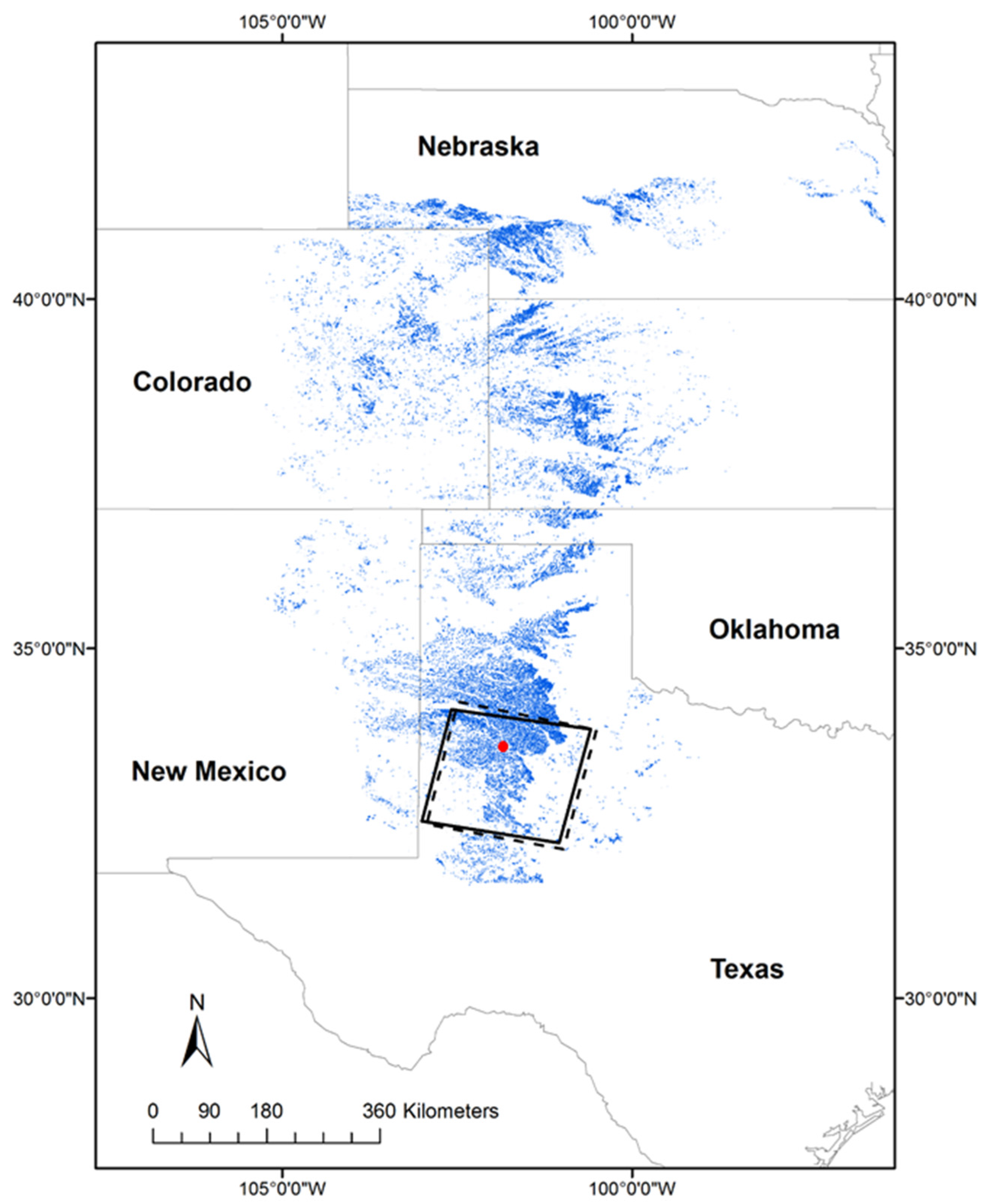
2.1. Study Area
2.2. Approach
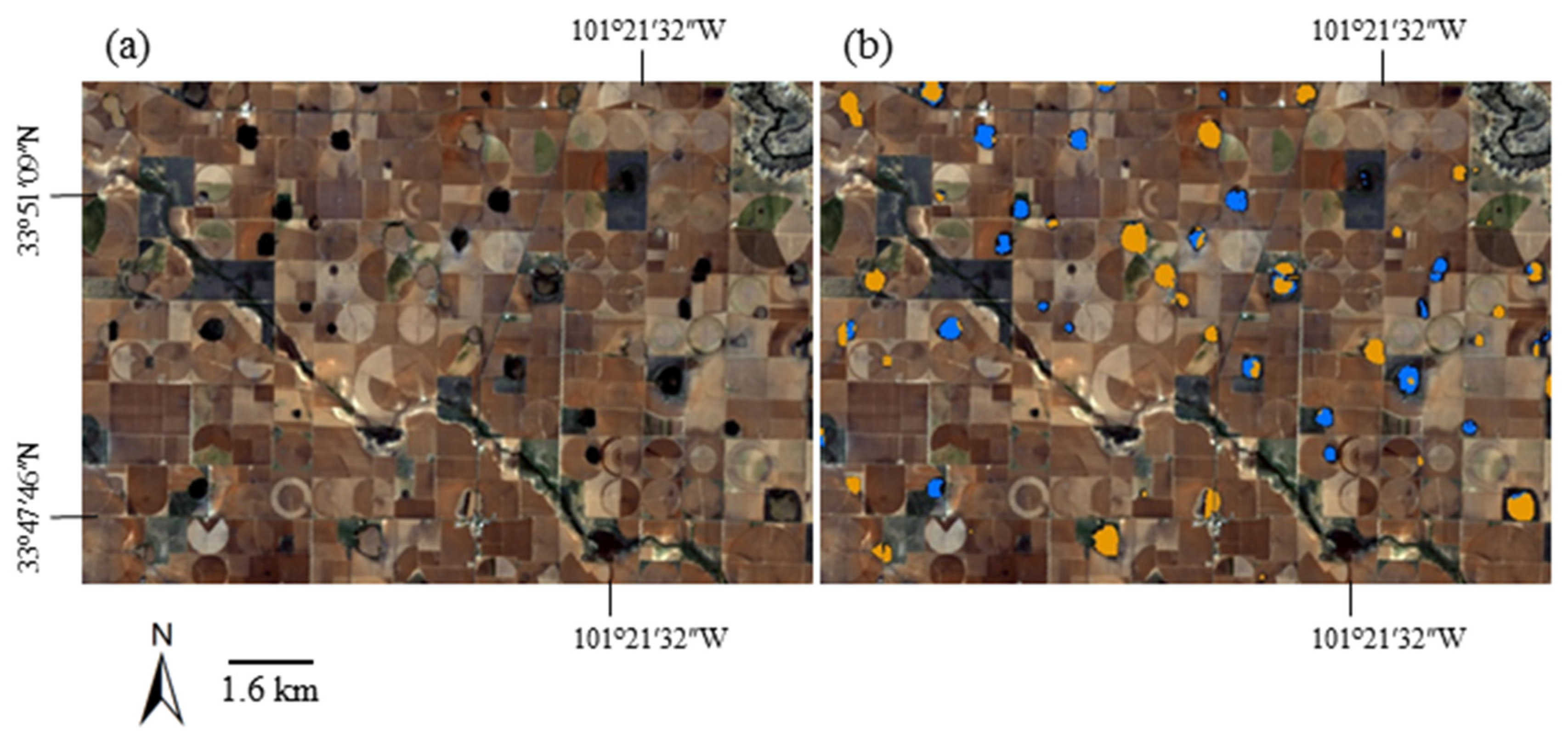
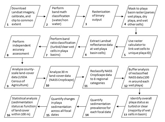
2.3. Methods
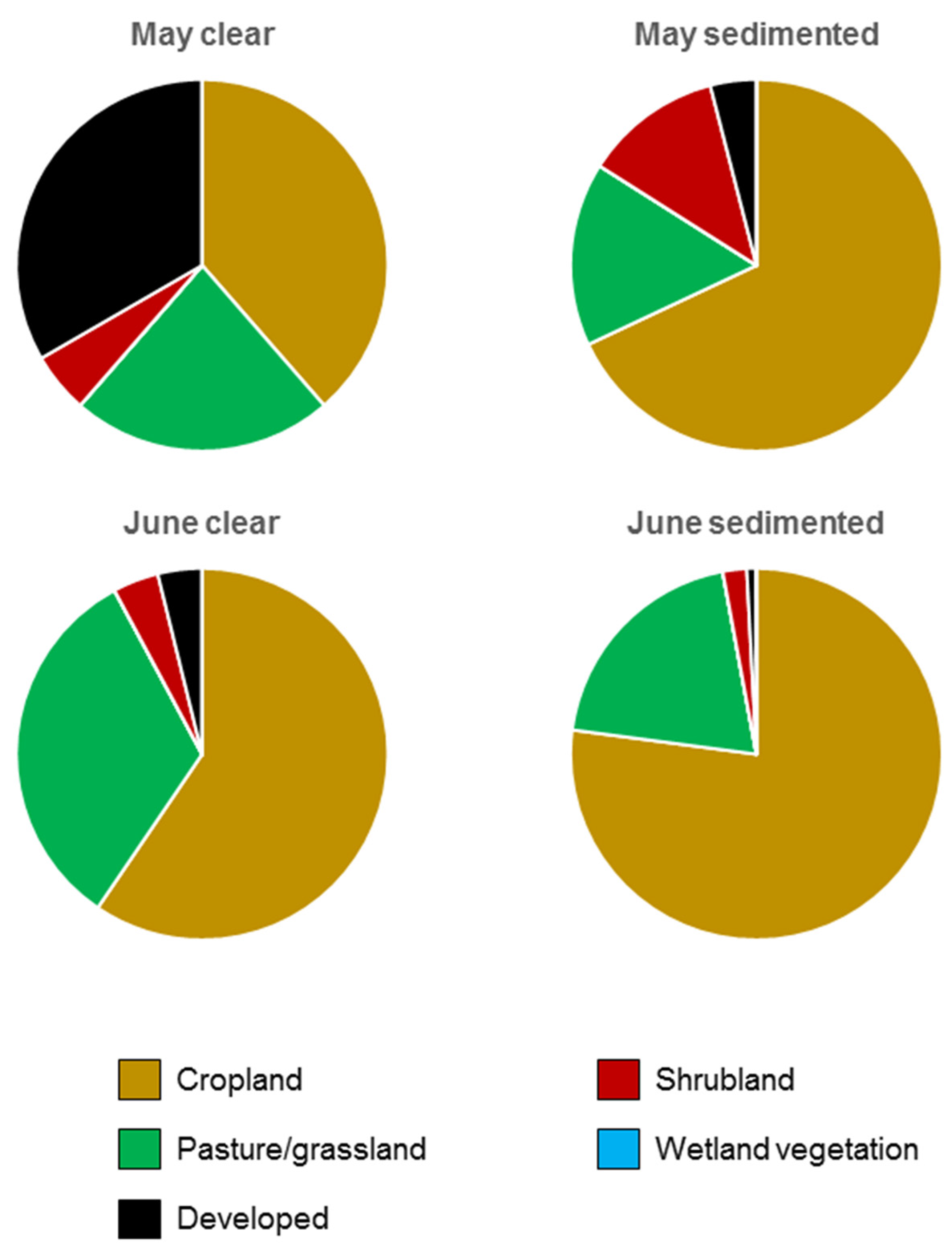
3. Results
4. Discussion
Uncertainties, Errors, and Accuracies
5. Conclusions
Acknowledgments
Author Contributions
Conflicts of Interest
References
- Ritchie, J.C. Sediment, fish, and fish habitat. J. Soil Water Conserv. 1972, 27, 124–125. [Google Scholar]
- Richter, B.D.; Braun, D.P.; Mendelson, M.A.; Master, L.L. Threats to imperiled freshwater fauna. Conserv. Biol. 1997, 11, 1081–1093. [Google Scholar] [CrossRef]
- Martin, D.B.; Hartman, W.A. The effect of cultivation on sediment composition and deposition in prairie pothole wetlands. Water Air Soil Pollut. 1987, 34, 45–53. [Google Scholar] [CrossRef]
- Daniel, D.W.; Smith, L.M.; Haukos, D.A.; Johnson, L.A.; McMurry, S.T. Land use and Conservation Reserve Program effects on the persistence of playa wetlands in the High Plains. Environ. Sci. Technol. 2014, 48, 4282–4288. [Google Scholar] [CrossRef] [PubMed]
- Bolen, E.G.; Smith, L.M.; Schramm, H.L., Jr. Playa lakes: Prairie wetlands of the Southern High Plains. BioScience 1989, 39, 615–623. [Google Scholar] [CrossRef]
- Haukos, D.A.; Smith, L.M. The importance of playa wetlands to biodiversity of the Southern High Plains. Landsc. Urban Plan. 1994, 28, 83–98. [Google Scholar] [CrossRef]
- Smith, L.M. Playas of the Great Plains; University of Texas Press: Austin, TX, USA, 2003. [Google Scholar]
- Yechieli, Y.; Wood, W.W. Hydrogeologic processes in saline systems: Playas, sabkhas, and saline lakes. Earth Sci. Rev. 2002, 58, 343–365. [Google Scholar] [CrossRef]
- Fraser, L.H.; Keddy, P.A. (Eds.) The World’s Largest Wetlands: Ecology and Conservation; Cambridge University Press: New York, NY, USA, 2005.
- Batzer, D.P.; Baldwin, A.H. (Eds.) Wetland Habitats of North America: Ecology and Conservation Concerns; University of California Press: Berkeley, CA, USA, 2012.
- Wright, C.K.; Wimberly, M.C. Recent land use change in the Western Corn Belt threatens grasslands and wetlands. Proc. Natl. Acad. Sci. USA 2013, 110, 4134–4139. [Google Scholar] [CrossRef] [PubMed]
- Bassi, N.; Kumar, M.D.; Sharma, A.; Pardha-Saradhi, P. Status of wetlands in India: A review of extent, ecosystem benefits, threats and management strategies. J. Hydrol. Reg. Stud. 2014, 2, 1–19. [Google Scholar] [CrossRef]
- Haukos, D.A.; Smith, L.M. Ecology of Playa Lakes. In Fish and Wildlife Leaflet 13.3.7, Waterfowl Management Handbook; U.S. Fish and Wildlife Service: Washington, DC, USA, 1992; pp. 1–7. [Google Scholar]
- United States Department of Agriculture, Natural Resources Conservation Service. Field Indicators of Hydric Soils in the United States; Version 7.0; Vasilas, L.M., Hurt, G.W., Noble, C.V., Eds.; United States Department of Agriculture, Natural Resources Conservation Service: Washington, DC, USA, 2010. [Google Scholar]
- Mason, R. The cotton kingdom and the city of Lubbock: South Plains agriculture in the postwar era. In Lubbock: From Town to City; Graves, L.L., Ed.; West Texas Museum Association: Lubbock, TX, USA, 1986; pp. 1–55. [Google Scholar]
- Luo, H.-R. Effects of Land Use on Sediment Deposition in Playas. Master’s Thesis, Texas Tech University, Lubbock, TX, USA, 1994. [Google Scholar]
- Collins, S.D.; Heintzman, L.J.; Starr, S.M.; Wright, C.K.; Henebry, G.M.; McIntyre, N.E. Hydrological dynamics of temporary wetlands in the southern Great Plains as a function of surrounding land use. J. Arid Environ. 2014, 109, 6–14. [Google Scholar] [CrossRef]
- USDA Census of Agriculture. Available online: http://www.agcensus.usda.gov (accessed on 22 October 2015).
- Haukos, D.A.; Smith, L.M. Past and future impacts of wetland regulations on playas. Wetlands 2003, 23, 577–589. [Google Scholar] [CrossRef]
- Musick, J.T.; Pringle, F.B.; Harman, W.L.; Stewart, B.A. Long-term irrigation trends—Texas High Plains. Appl. Eng. Agric. 1990, 6, 717–724. [Google Scholar] [CrossRef]
- Tsai, J.-S.; Venne, L.S.; McMurry, S.T.; Smith, L.M. Influences of land use and wetland characteristics on water loss rates and hydroperiods of playas in the Southern High Plains, USA. Wetlands 2007, 27, 683–692. [Google Scholar] [CrossRef]
- O’Connell, J.L.; Johnson, L.A.; Daniel, D.W.; McMurry, S.T.; Smith, L.M.; Haukos, D.A. Effects of agricultural tillage and sediment accumulation on emergent plant communities in playa wetlands of the U.S. High Plains. J. Environ. Manag. 2013, 120, 10–17. [Google Scholar] [CrossRef] [PubMed]
- Tang, Z.; Gu, Y.; Drahota, J.; LaGrange, T.; Bishop, A.; Kuzila, M.S. Using fly ash as a marker to quantify culturally-accelerated sediment accumulation in playa wetlands. J. Am. Water Resour. Assoc. 2015. [Google Scholar] [CrossRef]
- Luo, H.-R.; Smith, L.M.; Haukos, D.A.; Allen, B.L. Sources of recently deposited sediments in playa wetlands. Wetlands 1999, 19, 176–181. [Google Scholar] [CrossRef]
- Luo, H.-R.; Smith, L.M.; Allen, B.L.; Haukos, D.A. Effects of sedimentation on playa wetland volume. Ecol. Appl. 1997, 7, 247–252. [Google Scholar] [CrossRef]
- Tsai, J.-S.; Venne, L.S.; McMurry, S.T.; Smith, L.M. Vegetation and land use impact on water loss rate in playas of the Southern High Plains. Wetlands 2010, 30, 1107–1116. [Google Scholar] [CrossRef]
- Daniel, D.W.; Smith, L.M.; McMurry, S.T. Land use effects on sedimentation and water storage volume in playas of the rainwater basin of Nebraska. Land Use Policy 2015, 42, 426–431. [Google Scholar] [CrossRef]
- Johnson, L.A.; Haukos, D.A.; Smith, L.M.; McMurry, S.T. Physical loss and modification of Southern Great Plains playas. J. Environ. Manag. 2012, 112, 275–283. [Google Scholar] [CrossRef] [PubMed]
- Johnson, L.A.; Haukos, D.A.; Smith, L.M.; McMurry, S.T. Loss of playa wetlands caused by reclassification and remapping of hydric soils on the Southern High Plains. Wetlands 2011, 31, 483–492. [Google Scholar] [CrossRef]
- Smith, L.M.; Haukos, D.A.; McMurry, S.T.; LaGrange, T.; Willis, D. Ecosystems services provided by playas in the High Plains: Potential influences of USDA conservation programs. Ecol. Appl. 2011, 21. [Google Scholar] [CrossRef]
- Burris, L.; Skagen, S.K. Modeling sediment accumulation in North American playa wetlands in response to climate change, 1940–2100. Clim. Chang. 2013, 117, 69–83. [Google Scholar] [CrossRef]
- Gitz, D.; Zartman, R.E.; Villarreal, C.J.; Rainwater, K.; Smith, L.M.; Ritchie, G. Sediment accumulation in semi-arid wetlands of the Texas Southern High Plains. Tex. J. Agric. Nat. Resour. 2015, 28, 70–81. [Google Scholar]
- Hall, D.L.; Sites, R.W.; Fish, E.B.; Mollhagen, T.R.; Moorhead, D.L.; Willig, M.R. Playas of the Southern High Plains: The macroinvertebrate fauna. In Invertebrates in Freshwater Wetlands of North America: Ecology and Management; Batzer, D.P., Rader, R.B., Wissinger, S.A., Eds.; John Wiley and Sons: New York, NY, USA, 1999; pp. 635–665. [Google Scholar]
- Kloiber, S.M.; Brezonik, P.L.; Bauer, M.E. Application of Landsat imagery to regional-scale assessments of lake clarity. Water Res. 2002, 36, 4330–4340. [Google Scholar] [CrossRef]
- Kloiber, S.M.; Brezonik, P.L.; Olmanson, L.G.; Bauer, M.E. A procedure for regional lake water clarity assessment using Landsat multispectral data. Remote Sens. Environ. 2002, 82, 38–47. [Google Scholar] [CrossRef]
- Brezonik, P.; Menken, K.D.; Bauer, M. Landsat-based remote sensing of lake water quality characteristics, including chlorophyll and colored dissolved organic matter (CDOM). Lake Reserv. Manag. 2005, 21, 373–382. [Google Scholar] [CrossRef]
- Olmanson, L.G.; Bauer, M.E.; Brezonik, P.L. A 20-year Landsat water clarity census of Minnesota’s 10,000 lakes. Remote Sens. Environ. 2008, 112, 4086–4097. [Google Scholar] [CrossRef]
- O’Dell, J.W. (Ed.) Method 180.1: Determination of Turbidity by Nephelometry; United States Environmental Protection Agency: Cincinnati, OH, USA, 1993.
- Henley, W.F.; Patterson, M.A.; Neves, R.J.; Lemly, A.D. Effects of sedimentation and turbidity on lotic food webs: A concise review for natural resource managers. Rev. Fish. Sci. 2000, 8, 125–139. [Google Scholar] [CrossRef]
- Jurik, T.W.; Wang, S.-C.; van der Valk, A.G. Effects of sediment load on seedling emergence from wetland seed banks. Wetlands 1994, 14, 159–165. [Google Scholar] [CrossRef]
- Gleason, R.A.; Euliss, N.H., Jr.; Hubbard, D.E.; Duffy, W.G. Effects of sediment load on emergence of aquatic invertebrates and plants from wetland soil egg and seed banks. Wetlands 2003, 23, 26–34. [Google Scholar] [CrossRef]
- Anderson, J.T.; Smith, L.M. Persistence and colonization strategies of playa wetland invertebrates. Hydrobiologia 2004, 513, 77–86. [Google Scholar] [CrossRef]
- Sublette, J.E.; Sublette, M.S. The limnology of playa lakes on the Llano Estacado, New Mexico and Texas. Southwest. Nat. 1967, 12, 369–406. [Google Scholar] [CrossRef]
- Scheffer, M. Multiplicity of stable states in freshwater systems. Hydrobiologia 1990, 200, 475–486. [Google Scholar] [CrossRef]
- Tsai, J.-S. Local and Landscape Factor Influences on Avian Community Composition in Playas of the Southern High Plains. Ph.D. Thesis, Texas Tech University, Lubbock, TX, USA, 2007. [Google Scholar]
- Gray, M.J.; Smith, L.M.; Leyva, R.I. Influence of agricultural landscape structure on a Southern High Plains amphibian assemblage. Landsc. Ecol. 2004, 19, 719–729. [Google Scholar] [CrossRef]
- Madej, M.A.; Wilzbach, M.; Cummins, K.; Ellis, C.; Hadden, S. The significance of suspended organic sediments to turbidity, sediment flux, and fish-feeding behavior. In Proceedings of the Redwood Region Forest Science Symposium: What Does The Future Hold? Albany, CA, USA, 2007; pp. 383–388.
- Lavery, P.; Pattiaratchi, C.; Wyllie, A.; Hick, P. Water quality monitoring in estuarine waters using the Landsat Thematic Mapper. Remote Sens. Environ. 1993, 467, 268–280. [Google Scholar] [CrossRef]
- Cox, R.M.; Forsythe, R.D.; Vaughan, G.E.; Olmsted, L.L. Assessing water quality in the Catawba River reservoirs using Landsat Thematic Matter satellite data. Lake Reserv. Manag. 1998, 14, 405–416. [Google Scholar] [CrossRef]
- Bustamante, J.; Pacios, F.; Díaz-Delgado, R.; Aragonés, D. Predictive models of turbidity and water depth in the Doñana marshes using Landsat TM and ETM+ images. J. Environ. Manag. 2009, 90, 2219–2225. [Google Scholar] [CrossRef] [PubMed]
- Odermatt, D.; Gitelson, A.; Brando, V.E.; Schaepman, M. Review of constituent retrieval in optically deep and complex waters from satellite imagery. Remote Sens. Environ. 2012, 118, 116–126. [Google Scholar] [CrossRef] [Green Version]
- National Weather Service. Available online: http://www.srh.noaa.gov/lub/?n=climate-klbb-pcpn (accessed on 22 October 2015).
- US Drought Monitor. Available online: http://droughtmonitor.unl.edu/ (accessed on 22 October 2015).
- Playa Lakes Joint Venture Playas Data Layer. Available online: http://pljv.org/PPv4_MapBook/probable_playas_v4_shapefiles.zip (accessed on 5 November 2015).
- USGS Global Visualization Viewer. Available online: http://glovis.usgs.gov (accessed on 25 October 2015).
- Ozesmi, S.L.; Bauer, M.E. Satellite remote sensing of wetlands. Wetl. Ecol. Manag. 2002, 10, 381–402. [Google Scholar] [CrossRef]
- Cariveau, A.B.; Pavlacky, D.C., Jr.; Bishop, A.A.; LaGrange, T.G. Effects of surrounding land use on playa inundation following intense rainfall. Wetlands 2011, 31, 65–73. [Google Scholar] [CrossRef]
- Playas and Wetlands Database. Available online: http://gis.ttu.edu/pwd (accessed on 25 October 2015).
- Mulligan, K.R.; Barbato, L.S.; Seshadri, S. Playas and Wetlands Database. Available online: http://gis.ttu.edu/pwd/PlayasDocument.pdf (accessed on 25 October 2015).
- Fish, E.B.; Atkinson, E.L.; Mollhagen, T.R.; Shanks, C.H.; Brenton, C.M. Playa Lakes Digital Database for the Texas Portion of the Playa Lakes Joint Venture Region; Texas Tech University: Lubbock, TX, USA, 1998. [Google Scholar]
- Sawaya, K.E.; Olmanson, L.G.; Heinert, N.J.; Brezonik, P.L.; Bauer, M.E. Extending satellite remote sensing to local scales: Land and water resource monitoring using high-resolution imagery. Remote Sens. Environ. 2003, 88, 144–156. [Google Scholar] [CrossRef]
- Alsdorf, D.; Lettenmaier, D.; Vörösmarty, C. The need for global, satellite-based observations of terrestrial surface waters. Eos Trans. Am. Geophys. Union 2003, 84, 275–276. [Google Scholar] [CrossRef]
- USDA National Agricultural Statistics Service CropScape. Available online: http://nassgeodata.gmu.edu/CropScape/ (accessed on 2 February 2015).
- Bartuszevige, A.M.; Pavlacky, D.C.; Burris, L.; Herbener, K. Inundation of playa wetlands in the western Great Plains relative to landcover context. Wetlands 2012, 32, 1103–1113. [Google Scholar] [CrossRef]
- Ruiz, L.J.; Parikh, N.N.; Heintzman, L.J.; Collins, S.D.; Starr, S.M.; Wright, C.K.; Henebry, G.M.; van Gestel, N.; McIntyre, N.E. Dynamic connectivity of temporary wetlands in the southern Great Plains. Landsc. Ecol. 2014, 29, 507–516. [Google Scholar] [CrossRef]
- Van der Kamp, G.; Hayashi, M.; Gallén, D. Comparing the hydrology of grassed and cultivated catchments in the semi-arid Canadian prairies. Hydrol. Process. 2003, 17, 559–575. [Google Scholar] [CrossRef]
- Van der Kamp, G.; Stolte, W.J.; Clark, R.G. Drying out of small prairie wetlands after conversion of the catchments to permanent brome grass. Hydrol. Sci. J. 1999, 44, 387–397. [Google Scholar] [CrossRef]
- Voldseth, R.A.; Johnson, W.C.; Gilmanov, T.; Guntenspergen, G.R.; Millett, B.V. Model estimates of land-use effects on water levels of northern prairie wetlands. Ecol. Appl. 2007, 17, 527–540. [Google Scholar] [CrossRef] [PubMed]
- Voldseth, R.A.; Johnson, W.C.; Guntenspergen, G.R.; Gilmanov, T.; Millett, B.V. Adaptation of farming practices could buffer effects of climate change on northern prairie wetlands. Wetlands 2009, 29, 635–647. [Google Scholar] [CrossRef]
- Skagen, S.K.; Melcher, C.P.; Haukos, D.A. Reducing sedimentation of depressional wetlands in agricultural landscapes. Wetlands 2008, 28, 594–604. [Google Scholar] [CrossRef]
- Johnston, C.A. Sediment and nutrient retention by freshwater wetlands: Effects on surface water quality. Crit. Rev. Environ. Control 1991, 21, 491–565. [Google Scholar] [CrossRef]
- Dosskey, M.G. Toward quantifying water pollution abatement in response to installing buffers on crop land. Environ. Manag. 2001, 28, 577–598. [Google Scholar] [CrossRef] [PubMed]


| Date | 25 July 1986 | 3 May 2014 | 4 June 2014 | 25 July 2015 |
|---|---|---|---|---|
| Satellite | Landsat 5 TM | Landsat 8 OLI | Landsat 8 OLI | Landsat 8 OLI |
| No. of playa basins present | 7921 | 8372 | 8372 | 8372 |
| No. of wet playas | 2128 | 82 | 2730 | 3015 |
| No. of turbid wet playas | 1270 | 25 | 1925 | 1553 |
| County | County Area (ha) | 1987 | 2012 | ||||||
|---|---|---|---|---|---|---|---|---|---|
| Total Cropland Area (ha) (%) | Irrigated Area (ha) (%) | Total Cropland Area (ha) (%) | Irrigated Area (ha) (%) | ||||||
| Borden | 234,653 | 25,575.32 | 10.90 | - | - | 25,519.90 | 10.88 | 2007.29 | 0.86 |
| Crosby | 233,617 | 121,676.02 | 52.08 | 33,981.78 | 14.55 | 121,241.00 | 51.90 | 45,231.98 | 19.36 |
| Dawson | 233,617 | 182,220.23 | 78.00 | 7621.46 | 3.26 | 194,738.00 | 83.36 | 24,758.70 | 10.60 |
| Gaines | 389,275 | 212,975.53 | 54.71 | 64,632.39 | 16.60 | 230,894.00 | 59.31 | 91,899.59 | 23.61 |
| Garza | 232,063 | 38,671.36 | 16.66 | 665.18 | 0.29 | 33,221.10 | 14.32 | 3284.41 | 1.42 |
| Hockley | 235,430 | 154,889.79 | 65.79 | 30,370.85 | 12.90 | 161,923.00 | 68.78 | 43,285.42 | 18.39 |
| Lamb | 263,661 | 162,683.22 | 61.70 | 72,161.11 | 27.37 | 189,924.64 | 72.03 | 72,653.62 | 27.55 |
| Lubbock | 233,358 | 166,144.10 | 71.20 | 50,090.69 | 21.47 | 171,518.00 | 73.50 | 62,940.08 | 26.97 |
| Lynn | 231,286 | 137,096.16 | 59.28 | 12,468.02 | 5.39 | 164,567.00 | 71.15 | 28,987.45 | 12.53 |
| Terry | 230,768 | 156,360.42 | 67.76 | 32,946.96 | 14.28 | 152,557.00 | 66.11 | 397,763.92 | 17.24 |
| County | 2012–1987 Total Cropland Area (ha) (%) | 2012–1987 Irrigated Area (ha) (%) | ||
|---|---|---|---|---|
| Borden | −55.44 | −0.02 | - | - |
| Crosby | −434.63 | −0.19 | 11,250.20 | 4.82 |
| Dawson | 12,517.33 | 5.36 | 17,137.24 | 7.34 |
| Gaines | 17,918.67 | 4.60 | 27,267.20 | 7.0 |
| Garza | −5450.31 | −2.35 | 2619.03 | 1.13 |
| Hockley | 7033.03 | 2.99 | 12,914.57 | 5.49 |
| Lamb | 27,241.38 | 10.33 | 492.51 | 0.18 |
| Lubbock | 5373.82 | 2.30 | 12,849.39 | 5.51 |
| Lynn | 27,471.28 | 11.88 | 16,519.43 | 7.14 |
| Terry | −3803.64 | −1.65 | 6829.96 | 2.96 |
© 2016 by the authors; licensee MDPI, Basel, Switzerland. This article is an open access article distributed under the terms and conditions of the Creative Commons by Attribution (CC-BY) license (http://creativecommons.org/licenses/by/4.0/).
Share and Cite
Starr, S.M.; Heintzman, L.J.; Mulligan, K.R.; Barbato, L.S.; McIntyre, N.E. Using Remotely Sensed Imagery to Document How Land Use Drives Turbidity of Playa Waters in Texas. Remote Sens. 2016, 8, 192. https://doi.org/10.3390/rs8030192
Starr SM, Heintzman LJ, Mulligan KR, Barbato LS, McIntyre NE. Using Remotely Sensed Imagery to Document How Land Use Drives Turbidity of Playa Waters in Texas. Remote Sensing. 2016; 8(3):192. https://doi.org/10.3390/rs8030192
Chicago/Turabian StyleStarr, Scott M., Lucas J. Heintzman, Kevin R. Mulligan, Lucia S. Barbato, and Nancy E. McIntyre. 2016. "Using Remotely Sensed Imagery to Document How Land Use Drives Turbidity of Playa Waters in Texas" Remote Sensing 8, no. 3: 192. https://doi.org/10.3390/rs8030192