1. Introduction
Unmanned aerial vehicle remote sensing (UAVRS) platforms are usually equipped with a charge-coupled device (CCD) digital camera for image acquisition, a global positioning system (GPS), and an inertial measurement unit (IMU) for observation of the platform position and attitude. Compared with traditional manned airborne remote sensing, the advantages of UAVRS are that it can work in high-risk situations and inaccessible areas without endangering human lives, and it can also capture higher-resolution images at a lower altitude. UAVRS is also suitable for cloudy weather conditions due to its ability to fly below the clouds [
1]. In the past decades, UAVRS has found various applications in many fields, such as three-dimensional (3D) mapping, forest and vegetation change monitoring, emergency management, and so on [
2,
3,
4].
However, UAVRS platforms are not as stable as large fixed-wing manned aircraft, and tend to move erratically during flight. This, coupled with the disorientation caused by long-term viewing of the system, makes the analysis of the image data problematic [
5]. The GPS and IMU equipped on a UAVRS system usually provide low-quality measurements, resulting in low-accuracy direct geolocation [
6], so indirect georeferencing using ground control points (GCPs) is often performed [
7]. With known ground coordinates of easily-identifiable image features, the EO parameters of UAVRS images can be solved through aerotriangulation bundle adjustment [
8]. However, GCP collection from field survey is often a costly procedure, and it may be difficult or even impossible for hazardous areas, such as scenes of earthquake and accidents.
Light detection and ranging (LiDAR) can directly generate a digital elevation model (DEM) and digital surface model (DSM) by using an interpolation method, and features more accurate measurement of points [
9,
10,
11,
12]. Since the positioning accuracy of LiDAR is much higher than that of UAVRS, a possible solution is to improve the UAVRS geo-positioning accuracy based on the integration of these two kinds of datasets. James (2006) and Liu (2007) presented methods of utilizing LiDAR data and its intensity images to provide GCPs for digital photogrammetry and orthorectification processes [
13,
14]. Barrand (2009) optimized photogrammetric DEMs using LiDAR-derived GCPs for glacier volume change assessment [
15]. LiDAR and photogrammetry are also complementary to each other, and thus the integration of both technologies is important in a number of remote sensing applications such as building extraction [
16], image classification [
17,
18,
19], 3D city modeling [
20,
21], and so on. The integration of LiDAR and photogrammetry is expected to produce more accurate and higher-quality products [
11].
An important issue for the integration of LiDAR data and UAVRS optical images is the registration of these two different types of datasets. In general, the existing registration methods can be classified into three types, as follows [
22].
(1) Registration based on a LiDAR intensity image. This turns the registration of 3D LiDAR data and 2D optical imagery into 2D image registration. However, LiDAR intensity images differ a lot from optical imagery in their gray-level properties and object description due to their very different processes of intensity recording, which makes it difficult to perform a direct similarity comparison between an optical image and a LiDAR intensity image. The property they share is the statistical similarity of the gray levels, and, hence, mutual information is employed to exploit the statistical dependencies between a LiDAR-derived intensity image and an optical imagery [
23,
24].
(2) Registration based on point clouds (
i.e., point sets). By dense matching and forward intersection, a mass of 3D points can be generated from optical images, thus transforming the problem into registration of two point sets [
25]. However, points acquired from optical images are mostly image features like breakpoints of texture or gray level, providing rich information along object space discontinuities and poor information along homogeneous surfaces with uniform texture, while LiDAR provides a discrete set of irregularly distributed points with rich information along homogeneous physical surfaces and poor information along object space discontinuities. The iterative closest point (ICP) algorithm is, therefore, required in the procedure of registration [
25,
26]. This procedure needs precise initial values for the iteration to avoid a local optimum. What is more, errors of image matching and forward intersection may be involved.
(3) Registration based on features. Feature-based registration utilizes corner points, lines, and planes as matching primitives [
27,
28,
29,
30,
31]. There are many algorithms for feature detection from optical imagery, such as Moravec, Förstner, SUSAN, Harris, and SIFT for corner detection [
32,
33,
34,
35,
36], and Canny, Sobel, and LOG for edge detection [
37,
38,
39]. However, considering the discreteness and irregularity, it is more complex to extract features from LiDAR point clouds, and the algorithms developed for LiDAR processing are not as mature as those for optical image processing [
27].
With respect to the aforementioned registration methods, the LiDAR intensity image based methods rely heavily on the quality and correctness of the intensity image, and a big difference between the LiDAR intensity image and the optical image can increase the registration difficulty and lead to registration failure. The 3D point cloud based methods may result in a local optimum if the initialization of the ICP algorithm is not precise enough. What is more, the quality of the 3D points generated from the optical images is always poor in the areas where sudden elevation changes occur, which may reduce the ultimate registration accuracy. The feature-based methods are relatively well suited for the registration of UAVRS optical images and airborne LiDAR data as they both contain enough distinctive and easily-detectable objects for the registration. There has been a considerable amount of research into feature-based registration [
6,
12,
13,
14,
15,
16,
20,
21,
22,
27,
28,
29,
30,
31], among which the point features are the most commonly used features, which can be attributed to their uniqueness and simplicity.
Compared with point features, linear features have advantages including [
40,
41]: (1) image space linear features are easier to extract with sub-pixel accuracy across the direction of the edge as they are discontinuous in one direction while point features are discontinuous in all directions; (2) linear features possess higher semantic information and geometric constraint are more likely to exist among linear features than points to reduce the matching ambiguity; and (3) linear features increase the redundancy and improve the robustness and geometric strength of photogrammetric adjustment. Therefore, Habib
et al. proposed a photogrammetric and LiDAR data registration method using linear features [
27,
28], where two alternative approaches were introduced. One directly incorporates the LiDAR lines as control in the photogrammetric bundle adjustment, the other is a two-step procedure starting with photogrammetric 3D model generation and followed by a similarity transformation using the photogrammetric and LiDAR common lines as control for absolute orientation. The two-step strategy is able to deal with multiple 3D datasets regardless of their origin, but the disadvantage is that the orientation parameters of the images still remain uncorrected in the photogrammetric datum which does not coincide with the LiDAR datum. In the one-step strategy, the image space lines are represented by a sequence of intermediate points along the feature to cope with image distortion. It has advantages when handling long linear features where image distortion may lead to deviations from straightness of the lines. For short linear features, the deviations caused by image distortion would be very small and may probably be overwhelmed by the extraction error of the intermediate points, especially if they are extracted manually. Therefore, in our study, only two points are used to represent a linear feature in image space which is interactively extracted using line detection algorithms. Also, semi-automation is achieved with the extraction of the object space linear features from LiDAR points. Moreover, Differing from the scenarios in most of the existing studies where only a few optical images were used for the registration with LiDAR data, and each image had adequate independent control features for the registration, in our study, the registration of 109 UAVRS images and airborne LiDAR data using 16 linear control features was investigated, which is expected to enrich the methodology for the registration of UAVRS optical images and airborne LiDAR data..
2. Methodology
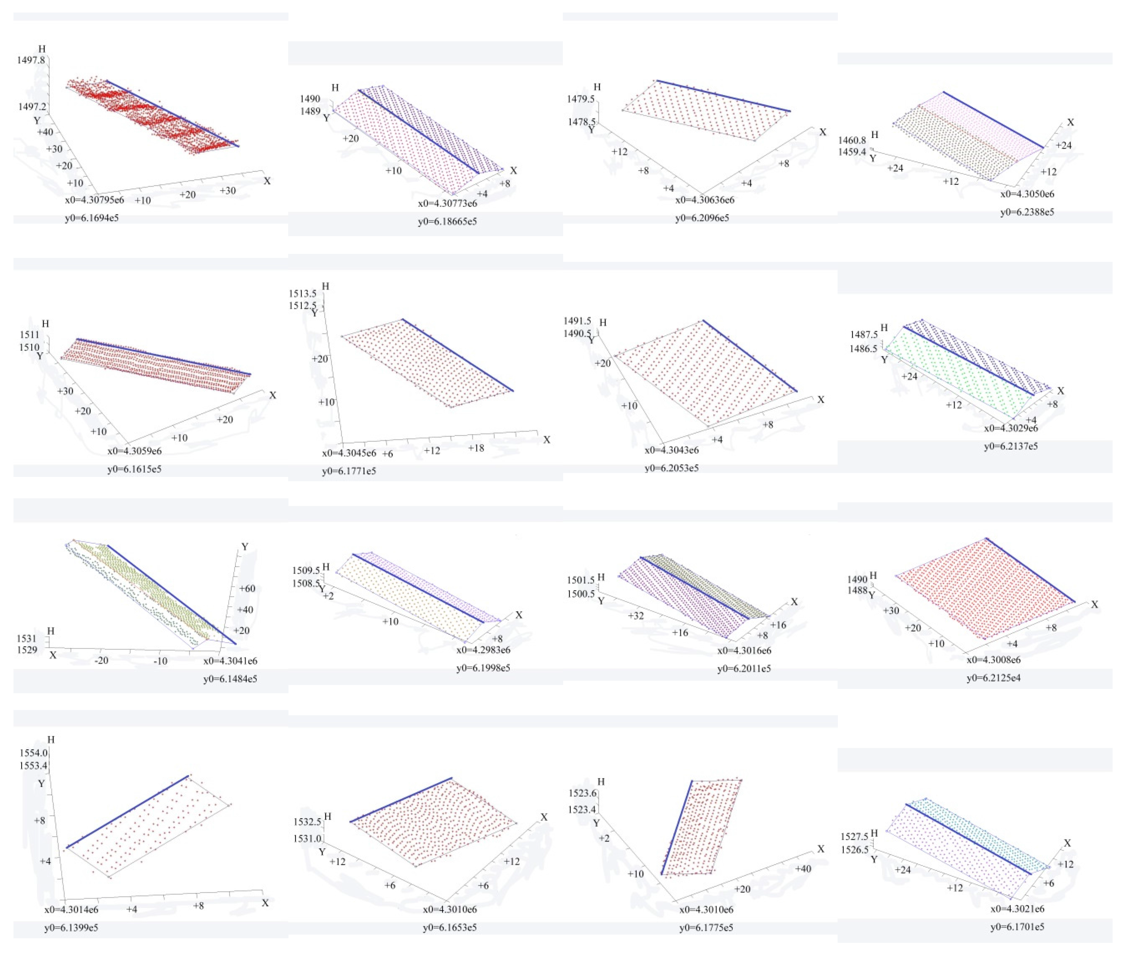
LiDAR data points are created as measurements in a 3D coordinate system. It is, therefore, convenient to take the coordinate system of the LiDAR data as the common framework, and the UAVRS images are then registered to the LiDAR data coordinate system. The registration involves the calculation of the EO parameters of the UAVRS images, which include the position of the exposure center (X0, Y0, Z0) and camera pose (ω, φ, κ). Planar roofs can be extracted from the LiDAR data with a high accuracy because a large amount of points can be applied to derive their parameters. Linear features subsequently derived from building roof edges and the intersection of adjacent planar roofs are used as control features. After block bundle adjustment using the coplanarity conditions derived from the linear control features and collinear conditions derived from a large number of tie points, the two datasets are registered in a common coordinate system.
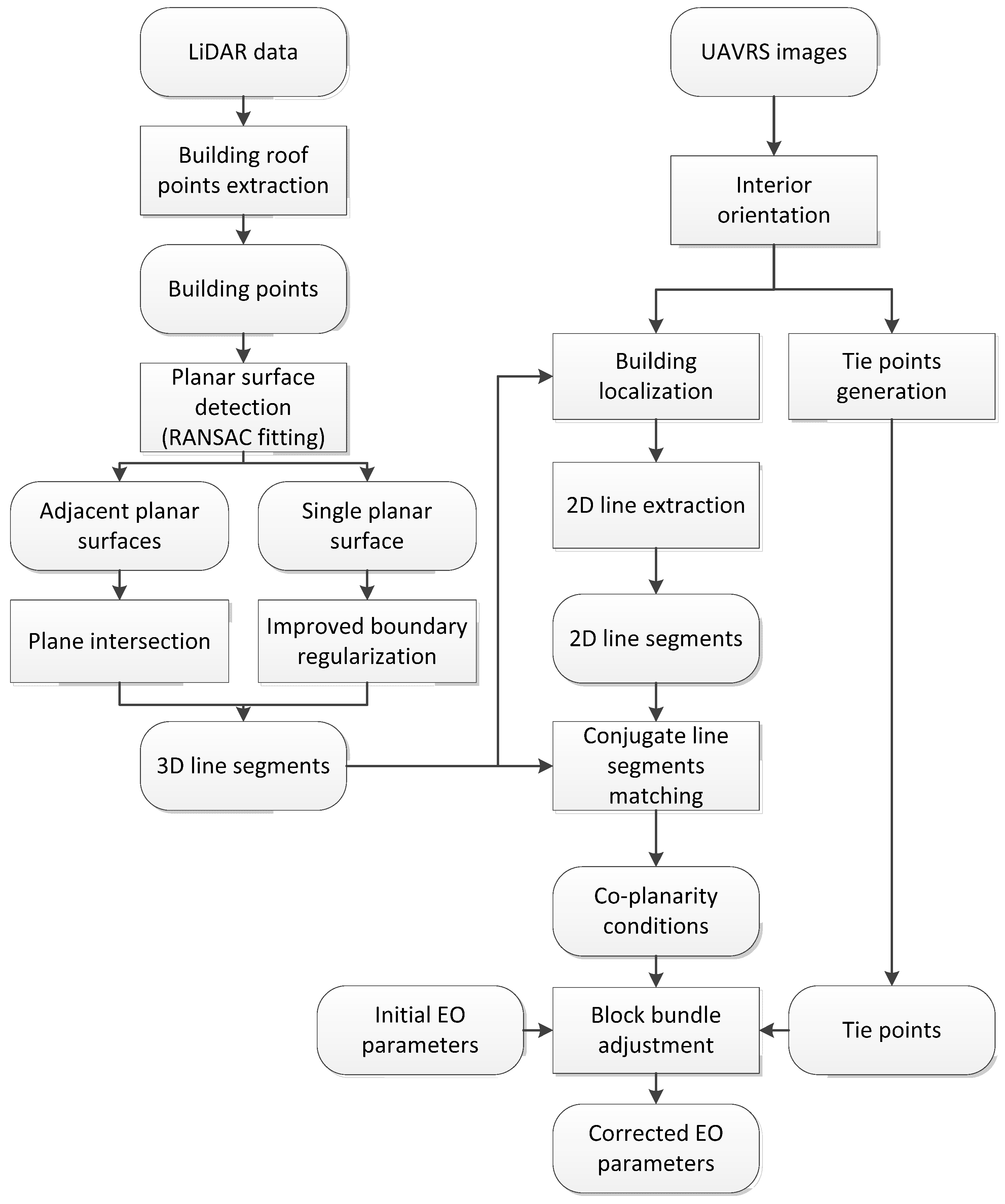
Figure 1 shows the overall workflow of the proposed method for the registration of UAVRS images and airborne LiDAR data. The approach consists of four main parts. (1) Buildings are separated from the LiDAR point cloud by the integrated use of height and size filtering and RANSAC plane fitting, and 3D line segments of the building ridges and boundaries are interactively extracted through plane intersection and boundary regularization; (2) the 3D line segments in the object space are projected to the image space using the initial EO parameters to obtain the approximate locations, and all the corresponding 2D line segments are semi-automatically extracted from the UAVRS images; (3) tie points for the UAVRS images are generated using a Förstner operator and least-squares image matching; and (4) based on the equations derived from the coplanarity constraints of the linear control features and the colinear constraints of the tie points, block bundle adjustment is carried out to update the EO parameters of the UAVRS images in the coordinate framework of the LiDAR data, achieving the co-registration of the two datasets.
Figure 1.
Overall workflow for the registration of UAVRS images and LiDAR data.
Figure 1.
Overall workflow for the registration of UAVRS images and LiDAR data.
2.1. Extraction of 3D Line Segments from LiDAR Data
2.1.1. Extraction of Building Roof Points
The airborne LiDAR data is processed in sequence. Firstly, pre-processing is performed to remove outliers. The remaining points are then divided into ground points and non-ground points. Building points are then extracted from the non-ground points, based on which the linear features are detected and extracted.
Outlier points include three types [
42]: isolated points, air points, and low points. With respect to the isolated points, the number of neighboring points according to a given 3D search radius is less than a predefined threshold. For air point detection, the mean value and standard deviation of the points′ elevations are first computed, and the points whose absolute elevation difference with the mean value is more than three times the standard deviation are considered to be air points. Low points are determined if their elevation is lower than all the neighboring points by a given threshold value (such as 1 m in our experiments).
After the outlier points are removed, the remaining points are further classified into ground and non-ground points using an adaptive triangulated irregular network (TIN) model [
43,
44]. The procedure is as follows: (1) seed point selection is undertaken in a user-defined grid with a size bigger than the largest building, and a coarse TIN is constructed; (2) new points are added in if they meet the criteria based on the calculated threshold parameters, and the TIN model is iteratively reconstructed; and (3) the procedure stops after all the points are checked and classified as ground or object. After the object points are separated from the ground points, building points are further extracted from the object points using height and size filtering [
12]. The thresholds used in our study for the experiment were 2.5 m for height and 3 m × 3 m for size.
2.1.2. Extraction of 3D Line Segments from Building Roof Points
In general, most buildings have regular shapes with perpendicular or parallel boundaries, and building roofs consist of one or more planes. There are three main methods for the detection of 3D building roof planes—region growing [
45], the Hough transform [
46], and RANSAC plane fitting [
47]—among which RANSAC is the most efficient while the region growing algorithms are sometimes not very transparent and not homogenous, and the Hough transform is very sensitive to the segmentation parameter values [
47]. Therefore, RANSAC plane fitting is adopted in our study for the roof plane detection and plane parameter estimation.
There are two types of line features that can be extracted from building roof points: roof ridge lines and roof edge lines. Roof ridge lines can be obtained by the intersection of adjacent roof planes for gable-roof buildings. However, boundary extraction from the irregular point set of a building roof is more complex. In this paper, a TIN-based algorithm is introduced to construct the boundary from the building roof points. The operational procedure of the algorithm includes three steps, as follows. (1) The building roof points are projected onto the X-Y 2D plane, and the TIN network is then constructed; (2) a threshold for edge length is determined based on the average point spacing (usually 2–3 times of the average spacing) and the edges longer than the threshold are removed; and (3) the edges that belong to only one triangle are selected to comprise the original building roof boundary.
The extracted original boundary is irregular, and further regularization is required to adjust the boundary to have a rectangular shape based on an orthogonal condition. Firstly, the main direction of the building is calculated, for which a method based on minimum direction difference is introduced. The direction difference is defined as the difference between each segment and the main direction. The optimal main direction is determined while the sum of all the direction differences is a minimum. The process of main direction detection is as follows. (1) Define the range of the main direction (0° ≤ < 90°), where αl changes from 0° to 90° with a given step of ε (ε = 90°/N, N is a given number to divide the range into N pieces); (2) in the ith iteration (i = 1, 2, …, N), calculate the direction difference for each edge segment. is defined as , in which is the azimuth of the jth edge segment, and all the s sum to ; and (3) complete the iterations, and the main direction is found when is the least.
After the main direction is determined, further regularization is performed to simplify the boundary to have a rectangular shape. (1) Segments are classified into two classes according to the difference between the azimuth of each line segment and the main direction. The result of this step is two groups of line segments, and they are supposed to be parallel or perpendicular to the main direction; (2) the connected segments of the same class are merged into a new edge line, and its weighted average of the center point and line azimuth are calculated. The weight used for each line segment is its length; and (3) the azimuth and location of each edge line are corrected by the use of an orthogonality constraint, and adjacent line segments of the regularized building boundaries will then be perpendicular to each other.
2.2. Extraction of Conjugate 2D Line Segments and Tie Points from UAVRS Images
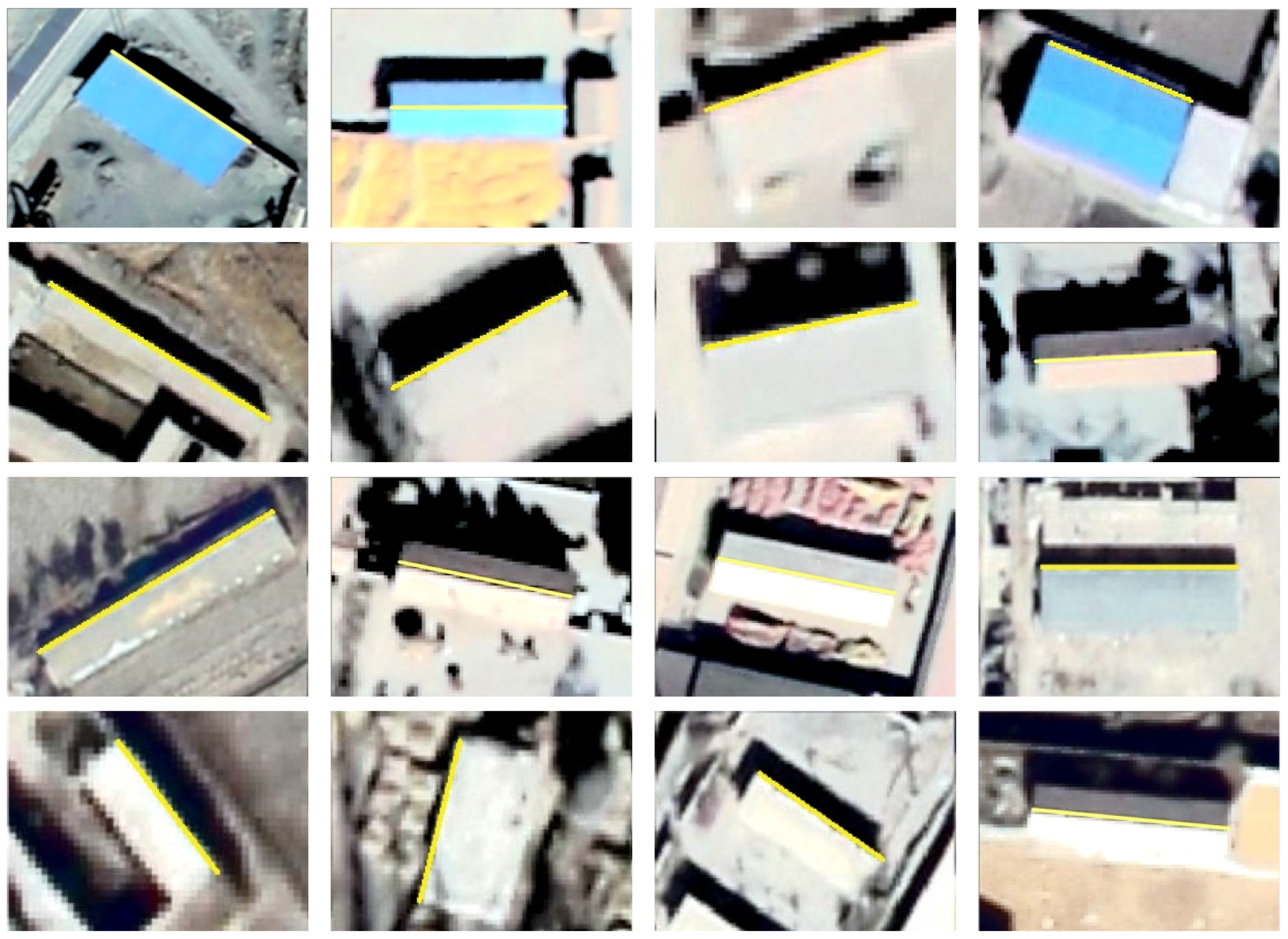
After the 3D line segments are extracted from the LiDAR points, the conjugate 2D line segments are interpreted from the UAVRS images in a semi-automatic way. Firstly, the extracted 3D ground line segments are projected to the image space using the interior orientation (IO) parameters and the initial EO parameters to determine the coarse location of the buildings to which the corresponding 2D line segments belong. The linear segments of the buildings are then automatically extracted using the Hough-transform algorithm [
48,
49], and the conjugate 2D line segments are then manually selected. There will be multiple (not less than two) conjugate 2D line segments in the image space for a 3D line segment in the ground space, and all the available 2D line segments are extracted. These conjugate 2D line segments also serve as tie features in bundle adjustment to reduce the geometric inconsistent between adjacent images.
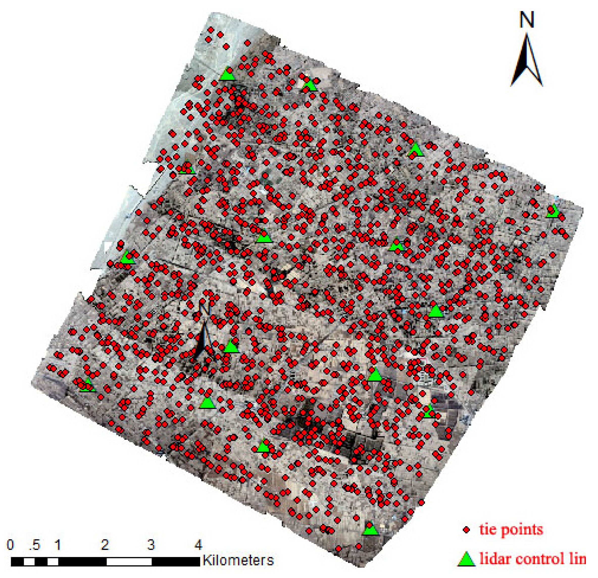
In addition to the 2D line segments used as a control, a large number of tie points is required for block bundle adjustment to reduce the geometric inconsistence between images and solve the EO parameters of all the UAVRS images. The tie points are automatically generated by use of the Förstner operator [
33] for feature point detection and least-squares image matching [
50] to establish the correspondence between conjugate points, for which geometric constraints such as epipolar constraint and parallax continuity constraint are applied to narrow the searching range and remove outliers.
2.3. Coplanarity Constraint of the Linear Control Features
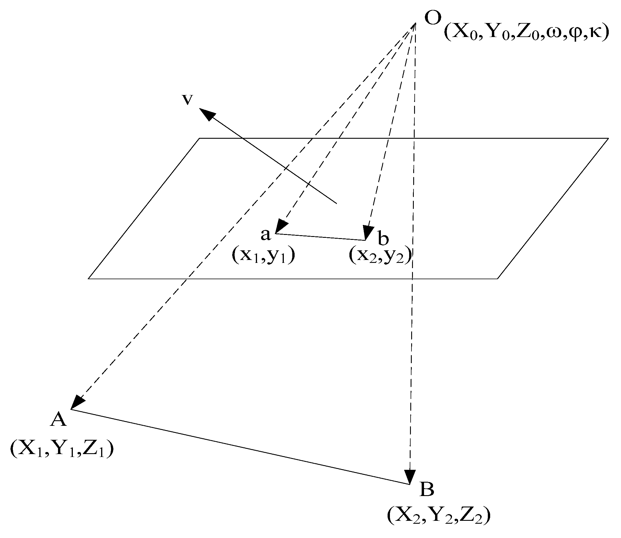
After the corresponding 2D and 3D line segments are extracted, registration can be carried out using the coplanarity condition [
12,
27]. As shown in
Figure 2, the 3D ground line segment A-B and its 2D conjugate line segment a-b in the image space are on the same plane, O-A-B, determined by the ground line A-B and the perspective center O. The advantage of using coplanarity is that no constraints are put on end points,
i.e., the end points of the corresponding line segments are not necessarily conjugate points.
Figure 2.
Coplanarity of corresponding 2D and 3D line segments.
Figure 2.
Coplanarity of corresponding 2D and 3D line segments.
In
Figure 2, the coplanarity condition of the five points, O, a, b, A, and B, is equivalent to the condition that both vectors
and
are perpendicular to the normal vector
of the plane determined by vectors
and
, which can be expressed as:
Each linear control feature provides two equations. For a single image, at least three linear control features (even distribution in image space preferable and should avoid being coplanar) are needed to solve the six unknown EO parameters. For a block of multiple overlapping images, tie points should be used to overcome the geometric inconsistency between adjacent images. Meanwhile, with the help of the tie points, the required minimum number of linear control features for the whole block of images is no more than that for a single image. However, for better accuracy, more than three well-distributed (evenly-distributed in plane and in elevation within the whole block area) linear control features are needed for redundancy checks and accuracy enhancement.
2.4. Block Bundle Adjustment
Each pair of corresponding line segments provides two independent equations, as indicated in Equation (1). For a block of n images, if we have m (m ≥ 3) pairs of linear control features evenly distributed in the entire block area, then we will have 2m equations provided by the coplanarity constraints and 6n unknown EO parameters. Meanwhile, if we have k tie points and each appears in four adjacent images (forward overlap and side overlap), they will provide 8k collinear equations and bring in 3k unknown ground coordinates.
Given the conditions above, we have 2m + 8k equations to solve the 6n + 3k unknowns, so (2m + 8k) should be no less than (6n + 3k), resulting in 2m + 5k ≥ 6n. The least-squares method is used for bundle adjustment to minimize the discrepancies among the conditions.
Initial values for the unknown parameters are required in bundle adjustment. The positions and attitudes measured by the onboard positioning and orientation system (POS) system are used as the initial values for the EO parameters of the images, and the initial ground coordinates for the tie points are calculated through space intersection using the initial EO parameter values. Both the EO parameter values of the images and the ground coordinates of the tie points are updated iteratively until the statistical error is less than the predefined threshold.
3. Study Area and Data Used
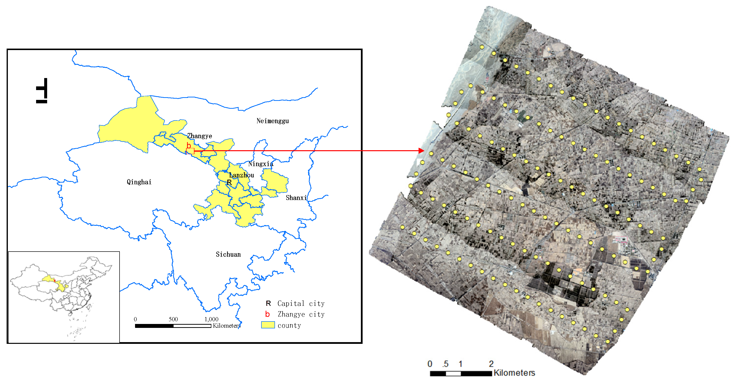
As shown in
Figure 3, the study area is located in Zhangye City, Gansu province, in the northwest of China, with an area of about 45 km
2. The topography in the study area is nearly flat, with an average elevation of 1550 m. The major land-cover types include farmland, trees, roads, and buildings, which are rich in linear features.
The UAVRS images used in the study were acquired in November 2011 and the UAV system used for image acquisition was ISAR-II, a fixed wing UAV equipped with a POS system including GPS and IMU for navigation and providing initial EO parameters for the acquired images, the detailed information could refer to [
51]. The accuracy of the attitude data from the IMU is rated as ±2° for roll and pitch and ±5° for heading. The technical specifications of the UAV are listed in
Table 1. The camera equipped on the UAV for image acquisition was a digital single lens reflex (DSLR) camera Canon EOS 5D Mark II, with single length of about 35.6 mm, recording images at a size of 5616 × 3744 pixels and pixel size is 6.41 μm. As the UAVRS mission was to provide geo-referenced image for the layout design of
in situ, sensors for the HiWATER (Heihe Watershed Allied Telemetry Experimental Research) project [
52], the required resolution was half meter. Therefore, considering the resolution requirement and the field condition (open country far away from flying restriction areas), in order to save the time for image acquisition and processing as much as possible, a flying height of 2500 m was designed for the image acquisition at an average resolution of 0.45 m, with overlapping of 65% along flight and 35% across flight respectively, and a total of 109 valid images were collected.
Figure 3.
The study area and the UAV flight path.
Figure 3.
The study area and the UAV flight path.
Table 1.
Technical specifications of the UAV platform used in the experiment [
51].
Table 1.
Technical specifications of the UAV platform used in the experiment [51].
| Item | Value |
|---|
| Length (m) | 1.8 |
| Wingspan (m) | 2.6 |
| Payload (kg) | 4 |
| Take-off-weight (kg) | 14 |
| Endurance (h) | 1.8 |
| Flying height (m) | 300–6000 |
| Flying speed (km/h) | 80–120 |
| Power | Fuel |
| Flight mode | Manual, semi-autonomous, and autonomous |
| Launch | Catapult, runway |
| Landing | Sliding, parachute |
The airborne LiDAR data for the same area were obtained by the use of a Leica ALS70 system onboard on an Y12 plane with flying height of about 1200 m in July 2012 [
53]. The average point density was four points per square meter and the vertical accuracy is 5–30 cm [
52]. In addition, 18 ground points, including road intersections and building corners, were surveyed using GPS-RTK with an accuracy better than 0.1 m, and served as checkpoints in the experiments.
5. Conclusions
Unmanned aerial vehicle remote sensing (UAVRS) has found applications in various fields, which can be attributed to its high flexibility in data acquisition and interpretable visual texture with the optical images. However, the platform instability and low accuracy of the position and attitude measurements result in big errors in direct georeferencing. As a complementary data source, LiDAR can provide accurate 3D information though is limited in object texture expression. Therefore, the integration of these two types of data is relevant and is expected to produce more accurate and higher-quality products, for which registration of the two different types of datasets is the first problem that needs to be solved. This paper has introduced a semi-automatic approach for the linear feature based registration of the UAVRS images and the airborne LiDAR data. Two aspects of the accuracy were assessed, one was the discrepancy between the two datasets after registration, which could be regarded as relative accuracy, and the other was absolute accuracy, which was assessed by comparing with the external GPS-surveyed points. From the experiments and result analysis, several conclusions can be drawn as follows.
(1) Compared with the traditional point based registration using the LiDAR intensity image, the linear feature based method directly using the LiDAR 3D data as control can provide a higher registration accuracy to the sub-pixel level, resulting in higher absolute accuracy in object space positioning. This could be attributed to the higher accuracy and geometric strength of the extracted linear control features from the LiDAR data than that of the control points from the LiDAR intensity image.
(2) The object space positioning error of the UAVRS images in the vertical is almost three times higher of that in the horizontal after registration with the LiDAR data in the experiment, which may be attributed to two aspects. One is the limited image overlapping of 65% along flight and 35% across flight, the other is that all the control features came from the line segments of the building roofs, while the check points included both the building roof points and the ground points. It could be expected that the vertical accuracy may be further improved if ground control features such linear features from roads were available in additional to the building control features.
(3) As the linear features mainly come from the manmade objects such as buildings and roads, the linear feature based registration strategy has advantages in urban areas, and is also applicable for the case with a reasonable coverage of algorithmically extractable linear features, but has limitations in a full natural environment, for which more investigation is needed for an effective solution.
(4) In spite of the advantages of the linear feature based registration strategy, automaticity in registration still remains an open problem and needs further study to improve the efficiency in practical applications, especially effort should focus on the automation with the extraction of common features from photogrammetric and LiDAR data, as well as the matching of the conjugate primitives.


 ,
, 


