Article

Quantifying the Daytime and Night-Time Urban Heat Island in Birmingham, UK: A Comparison of Satellite Derived Land Surface Temperature and High Resolution Air Temperature Observations

by
Juliana Antunes Azevedo
,
Lee Chapman
* and
Catherine L. Muller
School of Geography, Earth and Environmental Sciences, University of Birmingham, Birmingham B15 2TT, UK
*
Author to whom correspondence should be addressed.
Remote Sens. 2016, 8(2), 153; https://doi.org/10.3390/rs8020153
Submission received: 13 October 2015 / Revised: 27 January 2016 / Accepted: 1 February 2016 / Published: 17 February 2016

Abstract

:
The Urban Heat Island (UHI) is one of the most well documented phenomena in urban climatology. Although a range of measurements and modelling techniques can be used to assess the UHI, the paucity of traditional meteorological observations in urban areas has been an ongoing limitation for studies. The availability of remote sensing data has therefore helped fill a scientific need by providing high resolution temperature data of our cities. However, satellite-mounted sensors measure land surface temperatures (LST) and not canopy air temperatures with the latter being the key parameter in UHI investigations. Fortunately, such data is becoming increasingly available via urban meteorological networks, which now provide an opportunity to quantify and compare surface and canopy UHI on an unprecedented scale. For the first time, this study uses high resolution air temperature data from the Birmingham Urban Climate Laboratory urban meteorological network and MODIS LST to quantify and identify the spatial pattern of the daytime and night-time UHI in Birmingham, UK (a city with an approximate population of 1 million). This analysis is performed under a range of atmospheric stability classes and investigates the relationship between surface and canopy UHI in the city. A significant finding of this work is that it demonstrates, using observations, that the distribution of the surface UHI appears to be clearly linked to landuse, whereas for canopy UHI, advective processes appear to play an increasingly important role. Strong relationships were found between air temperatures and LST during both the day and night at a neighbourhood scale, but even with the use of higher resolution urban meteorological datasets, relationships at the city scale are still limited.

Graphical Abstract

1. Introduction

1.1. Background

The Urban Heat Island (UHI) continues to be a widely researched phenomenon concerning the difference in temperature between an urban area and the rural surroundings of a conurbation. A range of factors contribute to the occurrence of the UHI; increased emissions of anthropogenic heat flux, changes to urban geometry and the replacement of vegetation cover by construction material (e.g., asphalt and concrete)—all of which directly change surface albedo, emissivity and evapotranspiration [1]. The result is that it is common to find urban–rural temperature differences in excess of 5–10 °C under “ideal” conditions (e.g., clear skies and light winds). In many cases, the UHI is strongest at night; for example, a study a Paris showed that the magnitude of the night-time UHI was up to 7 °C more than the daytime UHI [2]. However, the daytime UHI is still a significant phenomenon, but is far more complicated to characterise. For example, it was found that urban temperatures tend to be slightly warmer than rural ones during the daytime in London with morning urban and rural temperatures being similar, but scenarios also exist where urban temperatures can be cooler than surrounding rural areas [3]. Systematic reviews of the UHI literature are available in [4,5] and both document a range of studies that have investigated both nocturnal and daytime temperature differences.
The UHI can impact many aspects of everyday life, such as critical infrastructure [6], health [7] and energy consumption [8], with impacts becoming exacerbated under heatwave events. For example, a study of the 2003 heat wave in Paris indicates that, at night-time, a surface temperature increase of ~0.5 °C could double the risk of elderly mortality [9]. Such events provide an indication of the increased impacts of the UHI in the increasingly warming climate projected to be experienced over the next few decades. Furthermore, the ever-increasing number of people in urban areas will not only further contribute to the exacerbation of the UHI effect, but will also increase the number of people exposed to its potential risks [10].
Studies into the UHI can be largely subdivided into three different types: the surface UHI (UHIsurface), the canopy UHI (UHIcanopy) and the boundary layer UHI (UHIboundary) [4,11]. The urban canopy is the thin layer of the atmosphere between ground level and roof top height and is strongly influenced by urban geometry and microscale energy exchange. The layer is just beneath the urban boundary layer [11] located above roof level and whose characteristics are affected by both mesoscale processes (i.e., prevailing wind) and the microscale processes below [1]. Air temperature (Tair) is the key parameter to measure for UHIcanopy and UHIboundary whereas land surface temperature (LST: often derived from satellites) is the parameter reported for UHIsurface. LST modulates the air temperature of lower layers, impacting on energy exchanges between the surface and air and therefore influences thermal comfort in the canopy layer as well as the internal climate of buildings [12].

1.2. Measuring the Urban Heat Island

Traditional ways in which UHIcanopy are measured include station pairs (e.g., [13]) or the use of transects (e.g., [10]). Given the paucity of traditional Tair observations, and their limited spatial resolution [10,14], there has been an ongoing challenge to quantify the intensity and spatial extent of the UHIcanopy. A compromise is nearly always needed, whether it be temporal (i.e., the transect approach) or spatial (i.e., the station pair approach). Techniques for measuring the UHIboundary are even more limited and rely on the use of tethered balloons, radiosondes or ground based remote sensing techniques [15].
It is for these reasons that numerical modelling techniques have proven to be so popular in urban climatology [16]. A range of models can be applied to estimate temperature variations in an urban area, such as the Weather Research and Forecasting model (WRF) [17], Joint UK Land Environment Simulator (JULES) [18], and the Met Office Reading Urban Surface Exchange Scheme (MORUSES) [3]. WRF is a mesoscale numerical weather prediction model, with incorporated urban schemes and used operationally for forecasting and research. JULES and MORUSES are land surface models that effectively provides information of land conditions (e.g., surface energy balance), which is subsequently passed on to atmospheric models, such as the Met Office Unified Model. Although modelling has brought tremendous advances in our understanding of urban atmospheric processes, models need observation data for initialisation and verification meaning that a wider number of urban measurements, other than data from one or two weather stations, would help to evaluate models’ output.
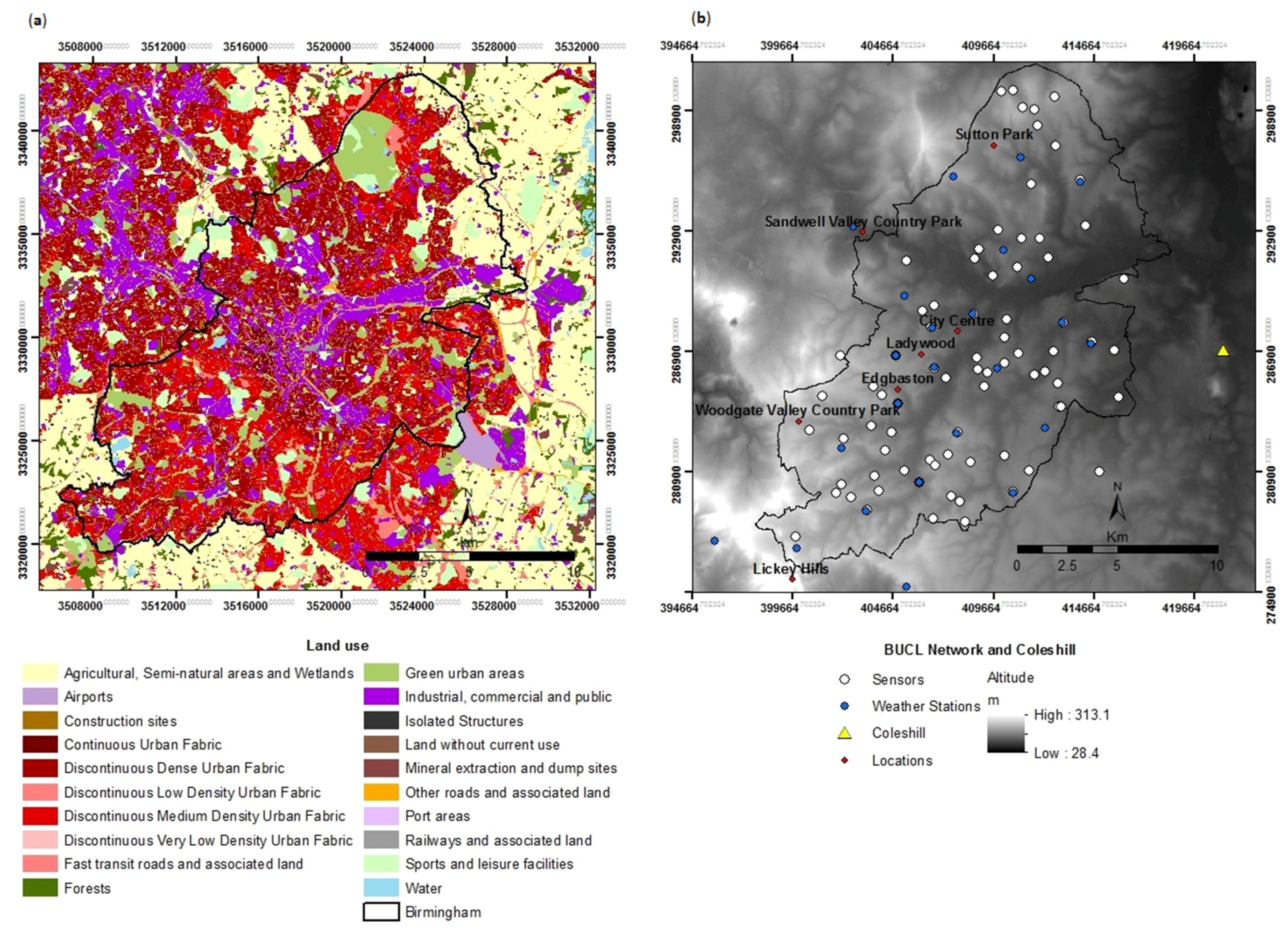
To this end, there has been a recent increase in interest in the deployment of high resolution Urban Meteorological Networks (UMNs) [19], driven by advances in technology, communications and the ever-increasing miniaturisation of low cost electronics [14]. Such networks enable atmospheric processes to be observed at both high temporal and spatial resolutions, which is especially important when considering the heterogeneous nature of urban areas [20]. Variables monitored by UMNs can include wind speed and direction, humidity, Tair and others. These data can be incorporated into microclimate models that can be further integrated into planning tools and other industrial applications to inform policy and decision-making. However, despite the advantages, the logistics of operating high resolution networks means that the number of fully working UMNs across the world is limited [14]. However, new approaches (e.g., crowdsourcing [21]) may help to improve this over time.
There are numerous studies in the literature that have quantified the UHIsurface using remote sensing techniques [9,10,22,23,24,25,26,27,28,29]. The key advantages being that regardless of the scale of study, remote sensing provides a consistent, repeatable and relatively cheap methodology for the end-user [7]. Although the initial cost of remote sensing platforms remains high, the data availability and temporal and spatial coverage available of LST measurements and other co-located variables (e.g., cloud, vegetation, surface emissivity) are important for UHIsurface measurements and spatial risk mapping [7,9,29].
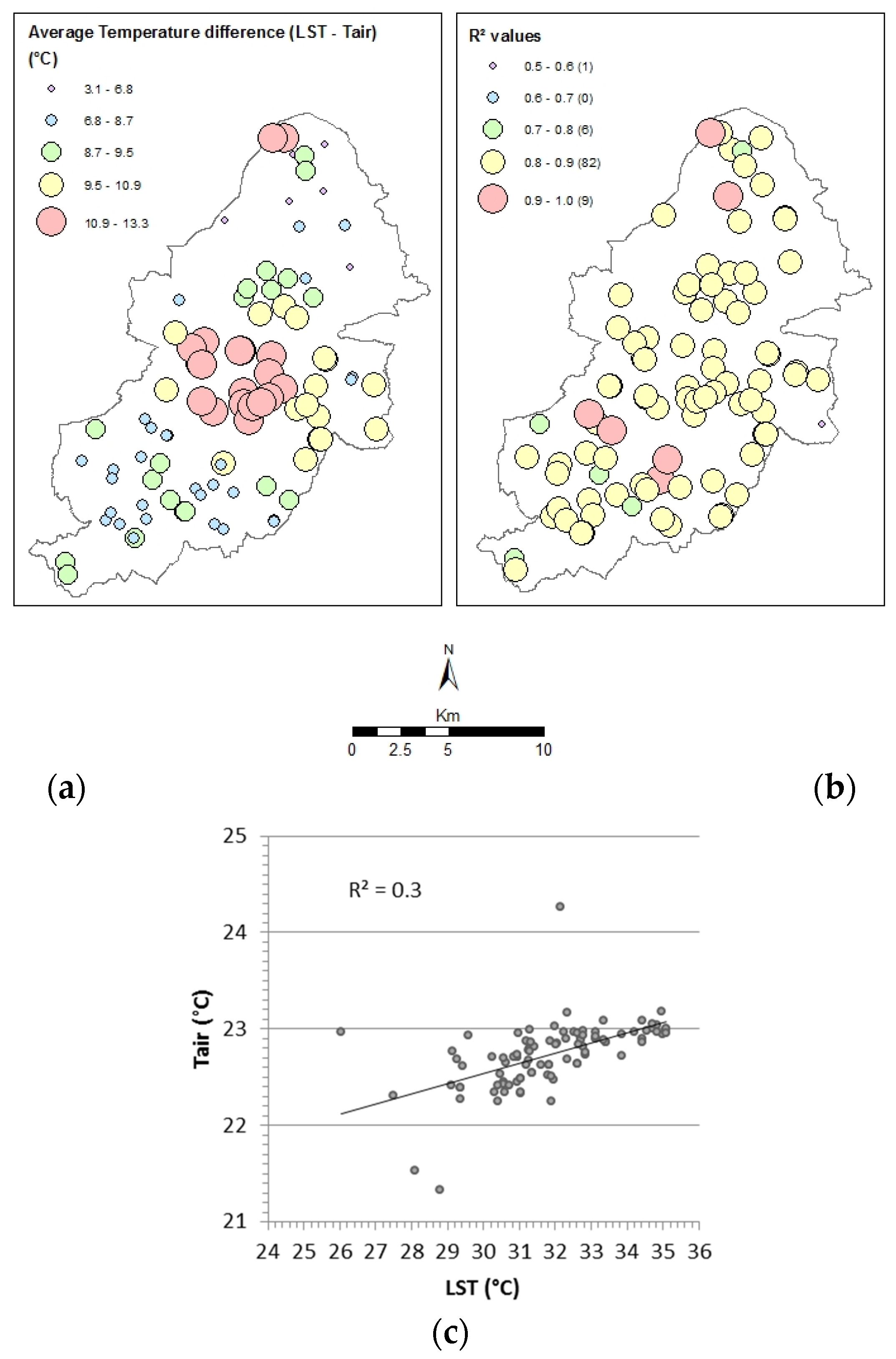
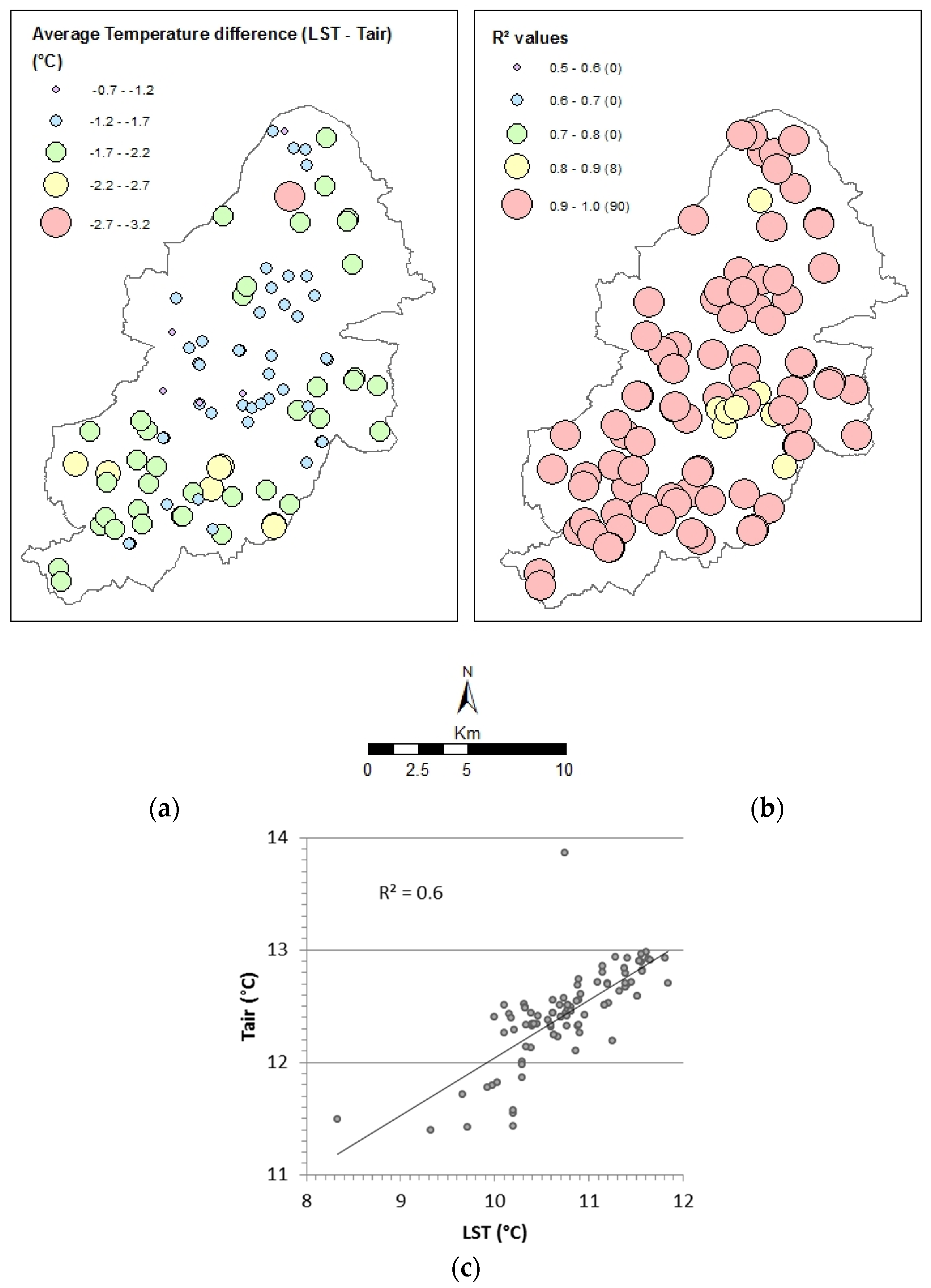
Despite the advantages, there are complexities in the retrieval of urban LST including satellite viewing geometry, atmospheric attenuation of IR radiation, urban surface emissivity and sub-pixel variations of land cover and heat balance. As a result, thermal remote sensing studies in urban areas had been slow on developing results beyond qualitative descriptions of thermal patterns and simple correlations between LST and Tair [12]. However, over the last decade, satellite derived LST were progressively integrated into climate models [30,31] and used to retrieve Tair [32]. To this end, the increasing availability of UMNs, of unprecedented resolution, have an important role to play. High resolution Tair datasets are not only providing new information on UHIcanopy but also provide an opportunity to further evaluate the relationship between Tair and LST using datasets of comparable spatial resolution. Furthermore, given the paucity of UMNs, this relationship is potentially useful allowing LST to be used in a wider range of applications that presently depend on Tair measurements (e.g., seasonal estimation of energy use [33] and electricity transformer ageing [34]). To begin to meet this need, this study uses a high resolution UMN (the Birmingham Urban Climate Laboratory: BUCL), to quantify and compare the spatial pattern of the daytime and night-time UHI in Birmingham-UK, under a range of stability classes, for both UHIsurface and UHIcanopy.

2. Study Area

Birmingham is the second largest city in the UK with an estimated population of over 1 million people [35]. It is a post-industrial city with a distinct range of landuse (e.g., the central business district, eastern industrial areas with the majority of residential areas straddling this belt of commerce and industry to the north and south). Some large parks can be found closer to the higher income neighbourhoods (Figure 1a). Altitude varies less than 100 m across the urban area (Figure 1b). The Lickey Hills, in the southwest corner of the city, provides the local highpoint and is the only notable topographical feature (297 m), which could exert a noticeable climate influence with respect to surface temperature lapse rates [36].
A number of studies have previously investigated the Birmingham UHI. Using night-time MODIS imagery for the summer of 2003–2009, it was identified that in periods of high atmospheric stability, the intensity of UHIsurface in Birmingham can reach up to 5 °C [23]. The cooling effect of green areas in Birmingham was also evident in this study, with notable cold spots in Sutton Park, Woodgate Valley and the Lickey Hills (Figure 1b). A significant LST gradient was observed extending northwards from the city centre to Sutton Park (~distance of 10 km) where temperatures can be 7–8 °C cooler than the urban core under heatwave conditions [34]. A further study investigated both the UHIcanopy (via station pairs) and MODIS UHIsurface of Birmingham in relation to Lamb Weather Types and identified that the strongest mean and maximum UHIcanopy and UHIsurface were during “ideal” anticyclonic conditions, reaching 7 °C and 4 °C, respectively [38]. Modelling approaches have also been used in the city with JULES showing a UHIcanopy of 4 °C under stable conditions [18] whereas the higher resolution WRF model, complete with an urban canopy scheme, highlighted a maximum intensity of 5.6 °C [17].
Figure 1b also shows BUCL: a near real time, high-resolution urban meteorological network of automatic weather stations and low-cost non-standard Wi-Fi air temperature sensors with bespoke radiation shields (Aginova Sentinel Micro) [20]. Data availability peaked in summer 2013, when the network consisted of: 82 air temperature sensors located in schools and on lampposts, 3 meters from the ground (see [20,39] for more details); and 25 automatic weather stations (Vaisala WXT520) measuring temperature, precipitation, relative humidity, wind speed and direction, pressure, solar radiation. Both temperature sensors and weather stations provide minute data. The weather stations provide accuracies of: air temperature ±0.3 °C (20 °C) [40] whereas the low-cost sensors provide good accuracy in laboratory testing with mean errors of <±0.22 °C (between −25 and 30 °C), subsequent field tests presented an accuracy (in the bespoke shield) of root-mean square error of 0.13 °C over a range of meteorological conditions relative to a traceable operational UK Met Office platinum resistance thermometer [39]. To ensure and improve data quality, a metadata protocol for UMNs was proposed and followed during implementation, maintenance and data acquisition. Furthermore, strict calibration procedures were rigorously followed (for detailed information see [19,39]). The network ensures Birmingham is one of the most densely-instrumented urban areas for meteorological studies and offers high quality data at an unprecedented resolution for a city of its size.
Finally, Coleshill (~4.5 km east of the outer edge of Birmingham), is the station in the national network frequently used as the rural reference site for UHI studies in Birmingham [23,38] and is considered an “agricultural, semi-natural and wetland” area in landuse classifications [37] (Figure 1a).

3. Methodology and Datasets

3.1. Tair Data Acquisition and Processing

Tair data for the study period was obtained from both BUCL [41] and Coleshill weather station. Twice daily meteorological averages were calculated for each sensor and weather station for daytime (06:00–17:59) and night-time (18:00–05:59 following day). Then, using ArcGIS, the data was interpolated by the Kriging Gaussian method before being averaged and trimmed to the study area, resulting in a daytime (representative of data averaged from 06:00 to 17:59) and night-time (18:00–05:59 the following day) interpolation for each day of the study period. Average values were used due to the rapidly changing nature of the UK climate. Although skies were clear during the time of the satellite passes used in this study, the proceeding weather conditions will potentially have a large impact. The use of averaging helps to overcome this limitation.
Kriging is commonly applied technique to interpolate Tair [42], and as with any interpolation method, there is the possibility of error. However, the larger the sample, the smaller the possible error; therefore, BUCL provides an improvement on estimations carried by Kriging by having a wider sample of data. Although it is possible that some stations might give anomalous readings, data from the network is carefully quality controlled by the technician enabling a reliable dataset for subsequent analysis [20]. A total of 82 sensors and 25 weather stations were used, which were functioning and reliable during the study period (including the sites outside the Birmingham urban area). The UHIcanopy intensity (Turban—Trural: in this case the difference between the interpolated Tair for the urban area and Tair in Coleshill) was then calculated. Finally, the daytime and night-time datasets were averaged according to Pasquill-Gifford stability classes (Table 1).

3.2. Pasquill-Gifford Stability Classes

Coleshill is the closest station in the national network (Met Office MIDAS WH hourly [43]) to Birmingham City Centre in which cloud observations are frequently made, crucial to enabling subsequent datasets to be classified into Pasquill-Gifford stability classes [44]. Daytime classes are calculated based on wind speed and levels of insolation (determined by cloud cover and solar elevation—Table 2 whereas night-time classes are calculated based on wind speed and cloud cover (Table 3). Meteorological data used to assign stability classes is from the rural reference site at Coleshill and, whilst it is assumed to be representative of regional conditions, there is a need to acknowledge atmospheric stability in the urban area could be different to that calculated.

3.3. LST Data Acquisition and Processing

Brightness data was acquired from the moderate-resolution imaging spectroradiometer (MODIS) which is deployed on board both the Terra and Aqua satellites. Birmingham overpass times for Terra are ~10:30 and ~22:30 whereas Aqua is between ~13:30 and ~01:30. During the British summer, sunset is between 20:00 and 22:00, with the maximum UHI being present ~3–5 h after sunset [1], making Aqua the ideal choice for analysis. Likewise, with respect to daytime observations, the Aqua satellite overpass at 13:30 should also provide a good reference since solar irradiance at the time is high (although it is accepted that this is not the time of maximum LST [30]). MODIS was selected over other platforms for its temporal resolution. Landsat TM offers a higher spatial resolution (60 m re-sampled to 30 m) [45], but the 16 days temporal resolution is prohibitive.
The freely available data product MYD11A1 (V5)—MODIS/Aqua Land Surface Temperature and Emissivity Daily L3 1km Grid SIN [46] was used. This product uses split window algorithms to correct for atmospheric effects [47] and surface emissivity [23]. Such data have been used in previous studies in Birmingham [23,48]. However, care needs to be taken during interpretation due to the split window technique that works well over homogeneous surfaces, but is not applicable to spatially variable urban surfaces.
Data was obtained for June, July and August (JJA) 2013 and was reprojected using the MODIS Reprojection Tool (MRT) [49] to convert images to GeoTIFF format at UTM, and subsequently converted to British National Grid (BNG) in ArcGIS (MODIS products are released in Sinusoidal Projection). Quality control of the images was also achieved in ArcGIS selecting only images that were 100% cloud free (i.e., whenever the image had a pixel with no value, the image was rejected), before converting LST from Kelvin to degree Celsius and trimming the images to the study area. Cloudiness is a recurrent problem in the UK, which significantly reduces data availability, which can sometimes be overcome by masking cloud on partially clear images. However, due to the spatial resolution of MODIS (1 km) and following an inspection of the nature of rejected images, the scientific gain of this additional processing was considered to be of limited value in this study, given the small increase in data such a step would provide.
The UHIsurface intensity (Turban—Trural: i.e., the pixel containing the Coleshill rural reference site) was then calculated. From each daytime and night-time image, the pixel LST converted to degree Celsius was extracted at the location of the sensor sites and weather stations (Figure 1b) for later comparison analyses between pixel extracted LST and sensor/weather station Tair. Finally, the images were averaged resulting in one daytime (at ~13:30) and one night-time (at ~01:30) image for each Pasquill-Gifford stability class.

4. Results

4.1. Stability Classification

Table 4 summarises the total number of images for daytime and night-time with respect to atmospheric stability. The difficulties in obtaining cloud free imagery in the study area becomes apparent with only 11 images for daytime and 13 images for night-time available for analysis during the study period. The image availability tends to increase with atmospheric stability for the night pass, whereas for daytime conditions the majority of imagery was available for the moderately unstable classes.
The Tair data was also classified using the same approach. By using this more extensive dataset, it can be seen that despite the settled climate experienced by the UK during the summer of 2013 (characterized by a mild heatwave and warmest temperatures since 2006), the most frequent stability classes encountered during the study period for the daytime were slightly unstable and moderately unstable. However, as per the LST data, more stable conditions were present at night.

4.2. Daytime UHIsurface

The averaged LST images for each stability class with sufficient LST imagery available are shown in Figure 2, accompanied with an average image representing the overall averaged dataset for the period, independently of stability class. A clear UHIsurface is evident across all stability classes, with LST in the city centre being several degrees warmer than Coleshill. The maximum difference recorded during this study was 9 °C (class B) and is comparable in magnitude to the 10 °C recorded in a study in Manchester, a similar sized conurbation in the north of the UK [10]. The clear spatial pattern found in all stability classes has peak LST in the land use classes for industrial, commercial and continuous urban fabric.
Significant cold spots are evident in city parks. LSTs recorded in the large Sutton Park to the north of the city are 9 °C lower than the city centre (~distance of 10 km) in class B, and 7–8 °C lower than the city centre in classes C and D respectively. In class B, Sutton Park was 1 °C lower than Coleshill (~distance of 15 km), and similar in classes C and D. In the southwest and northeast corners of the city, lower temperatures were also found and correspond to semi-rural areas with agricultural, semi-natural and wetland landuse. These differences are particularly noticeable in the southwest border where the slightly increased altitude has a discernable effect especially in Class B. Indeed, it is under these moderately unstable conditions that the maximum daytime UHIsurface is present. This finding is not unique to this study, with a maximum daytime temperature difference of 8.9 °C also occurring during partially cloudy periods in London, UK [50].
Overall, the results show a strong daytime UHIsurface, with peak temperatures corresponding to high urban density and lower temperatures in green areas across all stability classes. This outcome is to be expected due to the fact that LST maximum occurs in hours of maximum solar irradiance. Differences in the spatial pattern across the stability classes are attributed to wind speed and cloud cover (as used for the stability class classification).

4.3. Daytime UHIcanopy

As with the UHIsurface during the day, the UHIcanopy is also more evident under unstable conditions (Figure 3). However, it is identified that with the exception of the city centre core in classes A (~0.3 °C) and D (~1.8 °C), Tair during the day is lower than the rural reference site (and up to ~−1.8 °C lower in green areas and southwest, north and northeast semi-rural areas). Furthermore, in contrast to the UHIsurface, the intensity of the UHIcanopy spatial pattern is much smaller (between 1.7 °C and −1.8 °C), a result in line with other studies (e.g., [22]).
The spatial distribution of Tair during the period shows some similarities with LST with the highest temperatures in the city centre and cooler temperatures in urban parks (Sutton Park and southwest corner). However, there is a marked difference with respect to the spatial distribution of urban heat on the Tair dataset with the thermal core extending to the east of the city. In contrast, the thermal core extends to the west for the LST dataset. Whilst this pattern could be explained by land use for LST (Figure 1a), as the Tair pattern extending to east becomes more evident as the atmosphere becomes more stable (A to D), it is hypothesised that advection may play a more significant role in the spatial pattern of UHIcanopy. In WRF model simulations for August 2003, temperature variations in Birmingham were attributed to the influence of a particular wind direction in which areas downwind became warmer (up to 2.5 °C) than those upwind [17]. Hence, this temperature pattern can be explained by the prevailing wind for the region which is south-westerly [51]. Similar results regarding advection have also been found for other cities. In London, the peak UHI intensity was found to be located northeast of the city centre, possibly explained by the prevailing south-westerly winds [52] and in Hungary, the spatial UHI pattern in both Szeged and Debrecen, was determined by the prevailing wind direction [53]. Rural weather stations in the Netherlands were also found to be approximately 1 °C warmer when the wind passed across nearby towns [54]. Overall, it appears advection plays an important role in investigating the pattern of UHIcanopy in the city, but this is beyond the scope of the present study.

4.4. Night-time UHIsurface

Previous work in Birmingham identifies an increase in the UHIsurface intensity with respect to atmospheric stability [23]. That study used a larger dataset (2003–2009) than that used in this paper (i.e., summer 2013), yet the spatial pattern remains broadly comparable. The range for class F is from −1 to 2.5 °C, and class G from −1.6 to 3.0 °C; whereas for this study the ranges for class F are −0.25 to 2.75 °C, and class G from −1 to 3 °C (Figure 4). During a heatwave event (class G) which occurred on 18 July 2006, the UHIsurface peaked >4.5 °C. Unfortunately, given the smaller time period of this study, insufficient data is available in this analysis to assess the decline in UHIsurface intensity for classes E and D.
Overall, the spatial pattern of the UHIsurface at night-time is very similar to daytime. LST in the city centre is higher (~3 °C) than Coleshill and in parks and southwest and northeast borders it is lower (up to −1 °C). As expected, UHI intensity during night-time is lower (−1 °C to 3 °C) than daytime during the times of maximum solar irradiance (−1 °C to 8.7 °C).

4.5. Night-Time UHIcanopy

As with night UHIsurface, UHIcanopy is most evident under stable conditions, with the greatest intensity and a particularly well developed urban core in class G [23]. The spatial distribution of Tair during night-time (Figure 5) is also very similar to that highlighted during the daytime, with the core of urban heat becoming less defined and spreading eastwards across the city, again highlighting the potential role of advection in the structure of the UHIcanopy. For example, an investigation of the London UHI using MORUSES examined the factors shaping the spatial and temporal structure of the London’s atmospheric boundary layer. It was found that whilst landuse is the dominant factor, even weak advection is sufficient to increase nocturnal temperatures downwind of built up areas [3].

5. Comparisons between Land Surface and Air Temperatures

Using the datasets presented in this paper, direct temperature differences (LST—Tair) and R2 (coefficient of determination) were calculated between LST and Tair for each sensor site and weather station (neighbourhood scale) and later combined to investigate the relationship at the city scale. Note that Tair and LST are intrinsically different measurements [9]. Tair represents the ambient temperature at 2 m above the surface and LST represents the surface radiant temperature averaged over a 1 km horizontal surface (including different levels within the canopy layer). The time lag between maximum LST and Tair depends mainly upon the physical characteristics of the surface and convection. Although a strong correlation between the datasets is not expected, general patterns are helpful to retrieve Tair from LST [30].

5.1. Daytime

Figure 6a shows large differences between LST and Tair data collected at the time of the satellite overpass. These differences vary with landuse (Table 5) and range from around 3 °C in suburban areas, to over 13 °C directly adjacent to the thermal core, further highlighting the significance of the different processes contributing to UHIsurface and UHIcanopy in these areas. For comparison, an intensive study of Los Angeles, using 44 meteorological stations and seven AVHRR images during three days in August 1984, indicates a 5.4 °C difference between radiant surface and air temperatures in the afternoon (standard deviation of 2.3 °C) [28].
The result is that up to 91% of the variation in Tair at sites across Birmingham can be explained by LST (Figure 6b). With a couple of outliers as exceptions (e.g., one sensor site with a R2 of 0.5), this relationship is consistent across the city at the neighbourhood scale. However, when the analysis is extended to cover all sites at the city scale, the results and relationship are not consistent, and highlights the challenges in producing a simple relationship between Tair and LST (Figure 6c).

5.2. Night-Time

Direct comparisons between Tair and LST at night, show that Tair is consistently higher than LST across the city, ranging from 0.7 to 3.2 °C (Figure 7a). Temperature differences again vary with landuse (Table 6) with the lowest temperatures differences between LST and Tair in the city centre, likely because of the increased thermal capacity of urbanised surfaces. In contrast, the largest differences are in areas with more vegetation (i.e., Sutton Park and Woodgate Valley Country Park).
Site specific R2 values are consistently high between the two datasets (R2 = 0.8–1) with less outliers than during the daytime (Figure 7b); 8 sensors ranged between 0.8 and 0.9, and 90 between 0.9 and 1. Furthermore, the relationship at the city scale is improved at night (Figure 7c) and is to be expected given the less complex radiation processes operating after sunset. These results are greatly improved from a previous pilot study in Birmingham that compared 13 MODIS night-time summer LST images with 28 low-cost, unshielded, iButton loggers. In this study, R2 values were not as consistently high (R2 = 0.5–0.9) and no clear spatial pattern in the results was found [48]. Similarly, they show improvement on transect studies in Szeged, Hungary which yielded correlations in the range of 0.6–0.7 depending on the size of the sample radius [55]. The improved results in this study in comparison to the previous one in Birmingham [48] and Szeged [55] are attributed to the improved quality controlled/assured Tair dataset derived from BUCL [20]. Therefore, it highlights the importance of metadata and specific protocols when deploying sensors. Furthermore, correlations in all of these studies could have been different if correction of vertical surfaces were included (see Figure 1a from [12] for further information). However, the aim was to observe direct correlations between the values.

6. Conclusions

This paper has compared the UHIsurface and UHIcanopy in Birmingham, UK using MODIS LST and a unique, high resolution, Tair dataset. The UHI is clearly present in both datasets, both day and night, and over a range of atmospheric stability classes. During the day, LSTs in the city can be up to several degrees warmer than the rural reference, with the greatest variations occurring in class B (moderately unstable) reinforcing the findings of other similar studies (e.g., [50]). During the night, UHI intensity increases in line with atmospheric stability and is greatest in class G. During both the day and night, the UHIsurface was greater than UHIcanopy.
A key finding of this work are the differences in the spatial patterns for UHIsurface and UHIcanopy. With respect to UHIcanopy, there is a tendency for a larger core of urban heat to spread to the east of the city, which is hypothesised to be a result of advective processes, in line with other published results [17]. In contrast, UHIsurface extends more to the west of the city, suggesting that the UHIsurface pattern is more clearly linked with landuse, and that advection does not play a significant role. This difference is particularly distinct at night, and underlines the need to use high resolution datasets to further investigate advective process in the urban canopy. To this end, the 25 BUCL weather stations equipped for measuring wind speed and direction provide data for future investigation of advection, including its pattern and intensity.
Although strong relationships were found between Tair and LST during both the day and night at a neighbourhood scale, it is clear that, even with higher resolution datasets such as BUCL, it is presently unlikely that a simple statistical model could be obtained between LST and Tair at the city scale. However, quality controlled higher spatial and temporal resolution Tair datasets remain an important way in evaluating and validating Tair physically derived from LST.
To conclude, it is clear that the use of high resolution data from UMNs greatly facilitates work of this nature, and given extended periods of study, then general relationships and physical process-based numerical models could become more realistic. Indeed, the greatest potential in this area perhaps comes from co-located IR surface temperature monitoring devices at BUCL sites. These will enable surface temperature to be measured in the same vertical profile as air temperature and will potentially enable unprecedented direct ground truthing of LST datasets. If used in sufficient numbers per pixel (i.e., 1 km), this approach will provide high quality data for comparison studies simplifying the complexities of the wider environment/variable Tair source areas contained within a pixel. Overall, as this study has shown, improvements in measuring Tair across the urban environment are beneficial to not only understanding UHIcanopy, but also UHIsurface.

Acknowledgments

The authors would like to thank the Brazilian agency CNPq (Brazilian National Council for Scientific and Technological Development—Research Grant: [236849/2012-3]) for their financial support of this research. The research would not have been possible without data from NASA, the U.S. Geological Survey, the UK Meteorological Office, the help of BUCL technician Elliott Warren, and Richard Bassett who contributed in the final stages of corrections with clarification and information regarding the models and advection processes. Finally, yet importantly, to the reviewers who have extensively engaged with this manuscript and helped to improve the work considerably.

Author Contributions

Juliana Antunes Azevedo analysed the data and wrote the manuscript. Lee Chapman contributed in discussing the results and the writing process. Catherine L. Muller contributed with suggestions and comments before submission process and was involved in setting up the BUCL network.

Conflicts of Interest

The authors declare no conflict of interest.

References

  1. Oke, T. Boundary Layer Climates, 2nd ed.; Methuen: London, UK, 1987; p. 289. [Google Scholar]
  2. Lac, C.; Donnelly, R.P.; Masson, V.; Pal, S.; Riette, S.; Donier, S.; Queguiner, S.; Tanguy, G.; Ammoura, L.; Xueref-Remy, I. CO2 dispersion modelling over paris region within the CO2-megaparis project. Atmos. Chem. Phys. 2013, 13, 4941–4961. [Google Scholar] [CrossRef]
  3. Bohnenstengel, S.I.; Evans, S.; Clark, P.A.; Belcher, S.E. Simulations of the london urban heat island. Q. J. R. Meteorol. Soc. 2011, 137, 1625–1640. [Google Scholar] [CrossRef]
  4. Arnfield, A.J. Two decades of urban climate research: A review of turbulence, exchanges of energy and water, and the urban heat island. Int. J. Climatol. 2003, 23, 1–26. [Google Scholar] [CrossRef]
  5. Stewart, I.D. A systematic review and scientific critique of methodology in modern urban heat island literature. Int. J. Climatol. 2011, 31, 200–217. [Google Scholar] [CrossRef]
  6. Chapman, L.; Azevedo, J.A.; Prieto-Lopez, T. Urban heat & critical infrastructure networks: A viewpoint. Urban Clim. 2013, 3, 7–12. [Google Scholar]
  7. Tomlinson, C.; Chapman, L.; Thornes, J.; Baker, C. Including the urban heat island in spatial heat health risk assessment strategies: A case study for Birmingham, UK. Int. J. Health Geogr. 2011, 10. [Google Scholar] [CrossRef] [PubMed] [Green Version]
  8. Santamouris, M.; Papanikolaou, N.; Livada, I.; Koronakis, I.; Georgakis, C.; Argiriou, A.; Assimakopoulos, D.N. On the impact of urban climate on the energy consumption of buildings. Sol. Energy 2001, 70, 201–216. [Google Scholar] [CrossRef]
  9. Dousset, B.; Gourmelon, F.; Laaidi, K.; Zeghnoun, A.; Giraudet, E.; Bretin, P.; Mauri, E.; Vandentorren, S. Satellite monitoring of summer heat waves in the paris metropolitan area. Int. J. Climatol. 2011, 31, 313–323. [Google Scholar] [CrossRef]
  10. Smith, C.; Webb, A.; Levermore, G.J.; Lindley, S.J.; Beswick, K. Fine-scale spatial temperature patterns across a UK conurbation. Clim. Chang. 2011, 109, 269–286. [Google Scholar] [CrossRef]
  11. Oke, T. The Heat Island of the Urban Boundary Layer: Characteristics, Causes and Effects; Springer Netherlands: Dordrecht, The Netherlands, 1995. [Google Scholar]
  12. Voogt, J.A.; Oke, T.R. Thermal remote sensing of urban climates. Remote Sens. Environ. 2003, 86, 370–384. [Google Scholar] [CrossRef]
  13. Wilby, R.L. Past and projected trends in london’s urban heat island. Weather 2003, 58, 251–260. [Google Scholar] [CrossRef]
  14. Muller, C.L.; Chapman, L.; Grimmond, C.S.B.; Young, D.T.; Cai, X. Sensors and the city: A review of urban meteorological networks. Int. J. Climatol. 2013, 33, 1585–1600. [Google Scholar] [CrossRef]
  15. Barlow, J.F. Progress in observing and modelling the urban boundary layer. Urban Clim. 2014, 10, 216–240. [Google Scholar] [CrossRef]
  16. Grimmond, C.S.B.; Blackett, M.; Best, M.J.; Barlow, J.; Baik, J.J.; Belcher, S.E.; Bohnenstengel, S.I.; Calmet, I.; Chen, F.; Dandou, A.; et al. The international urban energy balance models comparison project: First results from phase 1. J. Appl. Meteorol. Climatol. 2010, 49, 1268–1292. [Google Scholar] [CrossRef]
  17. Heaviside, C.; Cai, X.M.; Vardoulakis, S. The effects of horizontal advection on the urban heat island in Birmingham and the West Midlands, United Kingdom during a heatwave. Q. J. R. Meteorol. Soc. 2015, 141, 1429–1441. [Google Scholar] [CrossRef]
  18. Bassett, R.; Cai, X.; Thornes, J.E.; Rees, R.; Chapman, L. Urban climatic map studies in UK: Birmingham. In The Urban Climatic Map: A Methodology for Sustainable Urban Planning; Edward, N., Chao, R., Eds.; Routledge: London, UK, 2015. [Google Scholar]
  19. Muller, C.L.; Chapman, L.; Grimmond, C.S.B.; Young, D.T.; Cai, X.M. Toward a standardized metadata protocol for urban meteorological networks. Bull. Am. Meteorol. Soc. 2013, 94, 1161–1185. [Google Scholar] [CrossRef]
  20. Chapman, L.; Muller, C.L.; Young, D.T.; Warren, E.L.; Grimmond, C.S.B.; Cai, X.M.; Ferranti, E.J.S. The Birmingham urban climate laboratory: An open meteorological testbed and challenges of the smart city. Bull. Am. Meteorol. Soc. 2014, 96, 1545–1560. [Google Scholar] [CrossRef]
  21. Muller, C.L.; Chapman, L.; Johnston, S.; Kidd, C.; Illingworth, S.; Foody, G.; Overeem, A.; Leigh, R.R. Crowdsourcing for climate and atmospheric sciences: Current status and future potential. Int. J. Climatol. 2015, 35, 3185–3203. [Google Scholar] [CrossRef]
  22. Roth, M.; Oke, T.R.; Emery, W.J. Satellite-derived urban heat islands from three coastal cities and the utilization of such data in urban climatology. Int. J. Remote Sens. 1989, 10, 1699–1720. [Google Scholar] [CrossRef]
  23. Tomlinson, C.J.; Chapman, L.; Thornes, J.E.; Baker, C.J. Derivation of birmingham’s summer surface urban heat island from modis satellite images. Int. J. Climatol. 2012, 32, 214–224. [Google Scholar] [CrossRef]
  24. Yuan, F.; Bauer, M.E. Comparison of impervious surface area and normalized difference vegetation index as indicators of surface urban heat island effects in landsat imagery. Remote Sens. Environ. 2007, 106, 375–386. [Google Scholar] [CrossRef]
  25. Weng, Q.; Lu, D.; Schubring, J. Estimation of land surface temperature-vegetation abundance relationship for urban heat island studies. Remote Sens. Environ. 2004, 89, 467–483. [Google Scholar] [CrossRef]
  26. Schwarz, N.; Lautenbach, S.; Seppelt, R. Exploring indicators for quantifying surface urban heat islands of european cities with MODIS land surface temperatures. Remote Sens. Environ. 2011, 115, 3175–3186. [Google Scholar] [CrossRef]
  27. Keramitsoglou, I.; Kiranoudis, C.T.; Ceriola, G.; Weng, Q.; Rajasekar, U. Identification and analysis of urban surface temperature patterns in greater Athens, Greece, using MODIS imagery. Remote Sens. Environ. 2011, 115, 3080–3090. [Google Scholar] [CrossRef]
  28. Dousset, B. Avhrr-derived cloudiness and surface temperature patterns over the los angeles area and their relationship to land use. In Proceedings of the IEEE Geoscience and Remote Sensing Symposium (IGARSS-89), Vancouver, BC, Canada, 10–14 July1989; pp. 2132–2137.
  29. Dousset, B.; Laaidi, K.; Zeghnoun, A. Surface temperature variability and mortality impact in the paris region during the august 2003 heat wave. Urban Clim. News 2011, 32, 7–14. [Google Scholar]
  30. De Ridder, K.; Bertrand, C.; Casanova, G.; Lefebvre, W. Exploring a new method for the retrieval of urban thermophysical properties using thermal infrared remote sensing and deterministic modeling. J. Geophys. Res. Atmos. 2012, 117, 1–14. [Google Scholar] [CrossRef]
  31. Wouters, H.; De Ridder, K.; Demuzere, M.; Lauwaet, D.; van Lipzig, N.P.M. The diurnal evolution of the urban heat island of paris: A model-based case study during summer 2006. Atmos. Chem. Phys. 2013, 13, 8525–8541. [Google Scholar] [CrossRef]
  32. Keramitsoglou, I.; Daglis, I.A.; Amiridis, V.; Chrysoulakis, N.; Ceriola, G.; Manunta, P.; Maiheu, B.; De Ridder, K.; Lauwaet, D.; Paganini, M. Evaluation of satellite-derived products for the characterization of the urban thermal environment. J. Appl. Remote Sens. 2012, 6, 061704. [Google Scholar] [CrossRef]
  33. Azevedo, J.A.; Chapman, L.; Muller, C.L. Critique and suggested modifications of the degree days methodology to enable long-term electricity consumption assessments: A case study in Birmingham, UK. Meteorol. Appl. 2015, 22, 789–796. [Google Scholar] [CrossRef]
  34. Tomlinson, C.J.; Prieto-Lopez, T.; Bassett, R.; Chapman, L.; Cai, X.M.; Thornes, J.E.; Baker, C.J. Showcasing urban heat island work in Birmingham—Measuring, monitoring, modelling and more. Weather 2013, 68, 44–49. [Google Scholar] [CrossRef]
  35. Birmingham City Council (BCC). B.C.C. Population in Birmingham. Available online: http://www.birmingham.gov.uk/ (accessed on 19 November 2014).
  36. Minder, J.R.; Mote, P.W.; Lundquist, J.D. Surface temperature lapse rates over complex terrain: Lessons from the cascade mountains. J. Geophys. Res. Atmos. 2010, 115, D14122. [Google Scholar] [CrossRef]
  37. European Environment Agency (EEA). Urban Atlas. Available online: http://www.eea.europa.eu/data-and-maps/data/urban-atlas#tab-figures-produced (accessed on 3 November 2015).
  38. Zhang, F.; Cai, X.; Thornes, J.E. Birmingham’s air and surface urban heat islands associated with lamb weather types and cloudless anticyclonic conditions. Prog. Phys. Geogr. 2014, 38, 431–447. [Google Scholar] [CrossRef]
  39. Young, D.T.; Chapman, L.; Muller, C.L.; Cai, X.M.; Grimmond, C.S.B. A low-cost wireless temperature sensor: Evaluation for use in environmental monitoring applications. J. Atmos. Ocean. Technol. 2014, 31, 938–944. [Google Scholar] [CrossRef]
  40. Scientific, C. Instructions wxt520 Weather Transmitter. Available online: https://s.campbellsci.com/documents/us/manuals/wxt520.pdf (accessed on 8 January 2016).
  41. Warren, E. Hitemp: High Density Meterological and Temperature Measurements within the Urban Birmingham Conurbation for the Hitemp Project; NCAS British Atmospheric Data Centre: London, UK, 2015. [Google Scholar]
  42. Chapman, L.; Thornes, J.E. The use of geographical information systems in climatology and meteorology. Prog. Phys. Geogr. 2003, 27, 313–330. [Google Scholar] [CrossRef]
  43. UKMO. U.M.O. Met Office Integrated Data Archive System (MIDAS) Land and Marine Surface Stations Data (1853-Current). Available online: http://badc.nerc.ac.uk/view/badc.nerc.ac.uk__ATOM__dataent_ukmo-midas (accessed on 19 November 2014).
  44. Pasquill, F.; Smith, F. Atmospheric Diffusion, 3rd ed.; Ellis Horwood Limited: Chichester, UK, 1983. [Google Scholar]
  45. USGS. U.S.G.S. Band Designation Landsat Satellites. Available online: http://landsat.usgs.gov/band_designations_landsat_satellites.php (accessed on 7 July 2014).
  46. USGS. U.S.G.S. Myd11a1 (v5)—Modis/Aqua Land Surface Temperature and Emissivity Daily l3 1 km Grid Sin. Available online: http://glovis.usgs.gov/ (accessed on 7 July 2014).
  47. LPDAAC. L.P.D.A.A.C. Modis Products Table—Myd11a1. Available online: https://lpdaac.usgs.gov/dataset_discovery/modis/modis_products_table/myd11a1 (accessed on 07 July 2014).
  48. Tomlinson, C.J.; Chapman, L.; Thornes, J.E.; Baker, C.J.; Prieto-Lopez, T. Comparing night-time satellite land surface temperature from modis and ground measured air temperature across a conurbation. Remote Sens. Lett. 2012, 3, 657–666. [Google Scholar] [CrossRef]
  49. LPDAAC. L.P.D.A.A.C. Modis Reprojection Tool. Available online: https://lpdaac.usgs.gov/tools/modis_reprojection_tool (accessed on 7 July 2014).
  50. Kolokotroni, M.; Giridharan, R. Urban heat island intensity in london: An investigation of the impact of physical characteristics on changes in outdoor air temperature during summer. Solar Energy 2008, 82, 986–998. [Google Scholar] [CrossRef]
  51. UKMO. U.M.O. Midlands: Climate. Available online: http://www.metoffice.gov.uk/climate/uk/regional-climates/mi (accessed on 21 April 2015).
  52. Chandler, T. Climate of London; W. Heffer & Sons, Ltd.: Cambridge, UK, 1965. [Google Scholar]
  53. Unger, J.; Sümeghy, Z.; Szegedi, S.; Kiss, A.; Géczi, R. Comparison and generalisation of spatial patterns of the urban heat island based on normalized values. Phys. Chem. Earth A/B/C 2010, 35, 107–114. [Google Scholar] [CrossRef]
  54. Brandsma, T.; Können, G.P.; Wessels, H.R.A. Empirical estimation of the effect of urban heat advection on the temperature series of de bilt (The Netherlands). Int. J. Climatol. 2003, 23, 829–845. [Google Scholar] [CrossRef]
  55. Unger, J.; Gal, T.; Rakonczai, J.; Mucsi, L.; Szatmari, J.; Tobak, Z.; van Leeuwen, B.; Fiala, K. Modeling of the urban heat island pattern based on the relationship between surface and air temperatures. Idöjárás 2010, 114, 287–302. [Google Scholar]
Figure 1. Birmingham—UK (a) Land use classes in Birmingham [37]; (b) Variation of altitude and location of laces mentioned in the text.
Remotesensing 08 00153 g001
Figure 2. Daytime UHIsurface intensity, for Pasquill-Gifford Stability Classes (B); (C) and (D); and Average for June, July, August 2013 and prevailing wind direction for the period. Based on MODIS Aqua LST product.
Remotesensing 08 00153 g002
Figure 3. Daytime UHIcanopy intensity, for Pasquill-Gifford Stability Classes (A); (B); (C) and (D); and Average for June, July, August 2013 and prevailing wind direction for the period. Based on the BUCL dataset.
Remotesensing 08 00153 g003
Figure 4. Night-time UHIsurface intensity, for Pasquill-Gifford Stability Classes (F) and (G), and Average for June, July, August 2013 and prevailing wind direction for the period. Based on MODIS Aqua LST product.
Remotesensing 08 00153 g004
Figure 5. Night-time UHIcanopy intensity, for Pasquill-Gifford Stability Classes (D); (E); (F) and (G); and Average for June, July, August 2013 and prevailing wind direction for the period. Based on the BUCL dataset.
Remotesensing 08 00153 g005
Figure 6. LST and Tair daytime comparison at 13:30. (a) LST—Tair difference (MODIS—BUCL); (b) R2 values at sensors and weather stations location; (c) R2 values for city scale (all sensors and weather stations).
Remotesensing 08 00153 g006
Figure 7. LST and Tair night-time comparison at 1:30. (a) LST—Tair difference (MODIS—BUCL); (b) R2 values at sensors and weather stations location; (c) R2 values for city scale (all sensors and weather stations).
Remotesensing 08 00153 g007
Table 1. Pasquill-Gifford Class Names.
ClassDefinition
AExtremely Unstable
BModerately Unstable
CSlightly Unstable
DNeutral
ESlightly Stable
FModerately Stable
GExtremely stable
Table 2. Insolation Categories for Pasquill-Gifford Day Stability Classes.
Sky CoverSolar Elevation
Angle > 60°35° > Angle < 60°15° > Angle < 35°
≤4/8 or any amount of high thin cloudsStrongModerateSlight
>4/8 middle clouds (700 foot—16,000 foot base)ModerateSlightSlight
>4/8 low clouds (less than 7000 foot base)SlightSlightSlight
Table 3. Pasquill-Gifford Stability Classes.
Surface Wind Speed (m·s−1)NightDay with Insolation
Cloud CoverInsolation
≥4/8 Oktas<4/8 OktasStrongModerateSlight
<2GGAA–BB
2–3EFA-BBC
3–5DEBB–CC
5–6DDCC–DD
>6DDCDD
Table 4. Pasquill-Gifford classification.
LST = 11 Daytime ImagesTair = 87 Days AnalysedPasquill-Gifford ClassDescription
012A and A-BExtremely Unstable
822B and B-CModerately Unstable
250C and C-DSlightly Unstable
13DNeutral
LST = 13 Night-Time ImagesTair = 86 Days AnalysedPasquill-Gifford ClassDescription
023DNeutral
019ESlightly Stable
313FModerately Stable
1031GExtremely stable
Table 5. Temperature difference (LST—Tair) at 13:30 and Land use [37].
Temperature Difference (°C)Land Use
10.9–13.3Industrial and commercial
9.5–10.9Continuous urban fabric; and discontinuous dense urban fabric
8.7–9.5Discontinuous low density urban fabric
6.8–8.7Discontinuous low density urban fabric
3.1–6.8Discontinuous low density urban fabric and green urban area
Table 6. Temperature difference (LST—Tair) at 1:30 and Land use [37].
Temperature Difference (°C)Land Use
−0.7–−1.2Industrial and commercial; continuous urban fabric; discontinuous dense urban fabric
−1.2–−1.7Industrial and commercial; continuous urban fabric; discontinuous dense urban fabric
−1.7–−2.2Discontinuous low density urban fabric; continuous and discontinuous urban fabric; and small proportion of industrial and commercial
−2.2–−2.7Discontinuous low density urban fabric and green urban area
−2.7–−3.2Green urban area

