Article

Diurnal Variability of Turbidity Fronts Observed by Geostationary Satellite Ocean Color Remote Sensing

1
State Key Laboratory of Satellite Ocean Environment Dynamics, Second Institute of Oceanography, State Oceanic Administration, 36 North Bao-Chu Road, Hangzhou 310012, China
2
State Key Laboratory of Tropical Oceanography, South China Sea Institute of Oceanology, Chinese Academy of Sciences, 164 Xingangxi Road, Haizhu District, Guangzhou 510301, China
3
University of Chinese Academy of Sciences, No. 19A Yuquan Road, Beijing 100049, China
*
Author to whom correspondence should be addressed.
Remote Sens. 2016, 8(2), 147; https://doi.org/10.3390/rs8020147
Submission received: 18 November 2015 / Revised: 23 January 2016 / Accepted: 4 February 2016 / Published: 16 February 2016
(This article belongs to the Special Issue Remote Sensing of Biogeochemical Cycles)

Abstract

:
Monitoring front dynamics is essential for studying the ocean’s physical and biogeochemical processes. However, the diurnal displacement of fronts remains unclear because of limited in situ observations. Using the hourly satellite imageries from the Geostationary Ocean Color Imager (GOCI) with a spatial resolution of 500 m, we investigated the diurnal displacement of turbidity fronts in both the northern Jiangsu shoal water (NJSW) and the southwestern Korean coastal water (SKCW) in the Yellow Sea (YS). The hourly turbidity fronts were retrieved from the GOCI-derived total suspended matter using the entropy-based algorithm. The results showed that the entropy-based algorithm could provide fine structure and clearly temporal evolution of turbidity fronts. Moreover, the diurnal displacement of turbidity fronts in NJSW can be up to 10.3 km in response to the onshore-offshore movements of tidal currents, much larger than it is in SKCW (around 4.7 km). The discrepancy between NJSW and SKCW are mainly caused by tidal current direction relative to the coastlines. Our results revealed the significant diurnal displacement of turbidity fronts, and highlighted the feasibility of using geostationary ocean color remote sensing technique to monitor the short-term frontal variability, which may contribute to understanding of the sediment dynamics and the coupling physical-biogeochemical processes.

Graphical Abstract

1. Introduction

Understanding oceanic fronts and their associated physical processes is essential for studying the exchange of water material and energy, ocean-atmosphere interaction, and marine ecosystems [1,2,3]. Because of the difficulty in observing the high dynamics of the front zones using traditional in situ measurements, satellite remote sensing with a high spatiotemporal resolution has been widely applied to analyze oceanic front distributions and their related biophysical processes around the world, based on the water mass differences of fronts in temperature and ocean color [4,5,6,7,8,9,10,11,12,13]. He et al. [14] showed that turbidity fronts coincide with thermal fronts in the Zhe-Min coastal waters of the East China Sea (ECS). However, thermal fronts are occasionally non-collocated with fronts in other properties (e.g., nutrients and salinity) [15,16,17]. Ocean color images, in contrast to thermal satellite data, can provide a more direct and accurate indication of the density gradients associated with physical processes [7,8,18,19], and can characterize seasonal and inter-annual variability [20,21,22,23]. Moreover, biophysical interaction and multi-scale physical processes (e.g., phytoplankton bloom, mesoscale eddies) are successfully visualized by combining thermal and ocean color fronts into a single map using visible and thermal satellite observations (e.g., Sea-Viewing Wide Field-of-View Sensor (SeaWiFS), The Advanced Very High Resolution Radiometer (AVHRR), and Moderate Resolution Imaging Spectroradiometer (MODIS)) [8,24,25,26,27]. The aforementioned studies have largely focused on the analysis of frontal frequency or averaged distributions using long-term or daily satellite images [4,8,28].
Few studies have been carried out on analysis of short-term frontal dynamics due to the limitation of conventional polar-orbiting satellite imagery with low to medium spatiotemporal resolutions (one or two scenes per day). Based on a constant efficiency model of the vertical mixing and infrared satellite imagery, Simpson and Bowers [29] described the variability of frontal displacements over a spring-neap tide in the United Kingdom shelf seas. Using two years of monthly sea surface temperature (SST) imagery, Paden et al. [30] found that advection rather than vertical mixing in the Gulf of California appears to be importance in the frontal displacement over the spring-neap tidal cycle. Using in situ acoustic Doppler current profiler (ADCP), conductivity, temperature, and depth (CTD), and mooring data, Kasai et al. [31] observed that the displacement of the thermohaline front in the Clyde Sea was dominated by tidal currents. Hopkins and Polton [32] used SST imagery and a regional numerical model to investigate the movement and structure of the thermohaline front in response to spring-neap tidal variability in the Liverpool Bay. In addition, using SST imagery and a one-dimensional model over a macrotidal continental shelf of Northern Patagonia Argentina, Pisoni et al. [33] found that the intensity variability of the San Matías and Valdés fronts was modulated by the spring-neap tidal transition. The conventional polar-orbiting satellite imagery, however, makes it difficult to identify high-frequency (e.g., hourly) frontal evolutions, especially in coastal waters. In contrast, the world’s first Geostationary Ocean Color Imager (GOCI), launched in 2010, can provide eight snapshots at a one-hour interval (i.e., from 00:15 to 07:45 GMT) with a high spatial resolution of 500 m [34]. Its unprecedented capability is of great benefit for the continuous monitoring of short-term finer oceanic phenomena and physical processes in near real time [35,36,37,38].
Various front detection methods that use remotely sensed images have been implemented to study oceanic front distributions and their temporal and spatial variability [4,5,6,7,8,9,10,11,12,13]. Compared with conventional gradient-based and histogram-based front detection algorithms used widely in oceanography [14,16,39,40], the automatic front detection technique based on Jensen–Shannon divergence (entropy-based algorithm) is more robust against noise and avoids previous filtering that would blur frontal features [11]. The entropy-based algorithm has already been used to retrieve the fine-scale SST fronts in different regions, such as the SST fronts near the Japanese coasts [11], the upwelling SST fronts in the Taiwan Strait and its surrounding waters [41,42], the inter-seasonal evolutions of fine-scale SST fronts in the northern South China Sea [43], and the SST front disappearance phenomena in the subtropical North Pacific [44].
In this study, taking two coastal regions called the northern Jiangsu shoal water (NJSW) and the southwestern Korean coastal water (SKCW) in the Yellow Sea (YS) as examples (Figure 1), we explored the capacity of applying GOCI to quantitatively monitor the diurnal displacement of water turbidity fronts. We applied the entropy-based algorithm to the GOCI-derived total suspended matter (TSM) instead of the traditional SST images, and retrieved the hourly turbidity fronts. Then, we analyzed the diurnal displacement of turbidity fronts in both the NJSW and SKCW. Moreover, the diurnal displacement of turbidity fronts during spring tide in NJSW was compared with it during neap tide to examine its response to spring-neap tidal changes. The reason for selecting NJSW and SKCW is that both of them have significantly diurnal variations of water turbidity mainly driven by tidal currents [38,45,46]. NJSW is located in a wide continental shelf with water depth less than 50 m and around 5001.7 km2 tidal flats [47]. A large amount of sediments had accumulated in the region due to the discharge of the old Yellow River for more than 700 years [48]. Its long-term turbidity featured with high temporal and spatial variability, mainly dominated by strong tidal currents and wind-induced vertical mixing, is frequently found based on satellite data and in situ measurements [46,48,49]. SKCW is characterized by narrow continental shelf with water depth less than 50 m and around 1036.9 km2 tidal flats [50]. In addition, SKCW is dominated by semi-diurnal tide with the duration of ebb tidal currents shorter than flood tidal currents [51].
Figure 1. Bathymetry (in meter) of the two studied regions, NJSW and SKCW, (black rectangular boxes) and their surrounding waters in the Yellow and East China Seas. “A” and “B” red points denote the tide gauge stations of “Dafeng-Harbor” and “Daeheuksando”, respectively. The black lines correspond to cross-front transects in each region.
Remotesensing 08 00147 g001

2. Data and Methods

2.1. GOCI Data Processing and Total Suspended Matter Retrieval

The GOCI acquires data eight times a day from 00:15 to 07:45 GMT with one-hour interval, with the coverage of about 2500 × 2500 km2 around the Korean Peninsula centered at 36°N and 130°E [38]. Here, two days of GOCI Level-1B data with cloudless condition on 5 April 2011 and 12 May 2015 were obtained from the Korea Ocean Satellite Center (KOSC), corresponding to the spring and neap tides, respectively. The GOCI Level-1B data were processed to retrieve hourly TSM using the GOCI data process software (GDPS) offered by KOSC. In the data processing, we used the KOSC standard atmospheric correction algorithm proposed by Ahn et al. [52,53]. In addition, the GOCI standard TSM algorithm (Yellow and East China Sea Ocean Color (YOC) algorithm) on the basis of Siswanto’s TSM retrieval model for the YS and ECS was used as follows [54,55]:
TSM ( mg / l ) = 10 ( 0 . 649 + 25 . 623 × ( R r s ( 555 ) + R r s ( 670 ) ) 0.646 × ( R r s ( 490 ) R r s ( 555 ) ) ) ,
where Rrs is the remote-sensing reflectance with unit of per steradian (sr−1). The YOC TSM algorithm was established and validated by extensive math-up data between in situ and GOCI observations covering NJSW and SKCW, with R2 = 0.87 and 35% of mean relative error [55].

2.2. Water Turbidity Front Retrieval

The GOCI-derived TSM data were then used to detect surface turbidity fronts using an effective algorithm based on Jensen–Shannon divergence (JSD), known as entropy-based algorithm [11]. The JSD method does not only diminish the influence of impulsive noise but also discerns the finer-scale curvilinear frontal features in coastal regions due to its independence from temporal or spatial variations of geophysical parameters [11]. Its effectiveness was already proven by Shimada et al. [11], and Chang and Cornillon [56] through comparison with other traditional methods (e.g., gradient magnitude and histogram edge detection algorithms) using the SST images, and the results showed that the entropy-based algorithm had better performance, especially for detecting short and weak fronts. Here, the JSD was calculated from four JSD matrices that were estimated in each of two 5 × 5 pixel TSM subwindows with four different directions (horizontal, vertical, and two diagonals, shown in [11]). The maximum of these four JSD matrices is regarded as the JSD value at each pixel. The calculated JSD value (termed “TSM–JSD”) ranges from zero to one, which is used to represent the spatial inhomogeneity of two neighboring TSM subwindows across a front, with a higher TSM–JSD corresponding to a stronger front. In this study, we took the pixels with a TSM–JSD greater than 0.4 as the frontal pixels, because smaller values cannot clearly express the curvilinear patterns [11,42].
Additionally, the TSM images were simultaneously applied to estimate sea surface currents using the well-known maximum cross-correlation (MCC) method [37,57]. Using GOCI-derived TSM sequential images, previous studies suggested that the MCC technique could be widely used to accurately derive high-frequency surface currents in the YS and ECS [37,58,59]. Specifically, we took a 10 × 10 km box centered with a certain pixel from one TSM image, and searched the location of the match-up box from the next sequential TSM image using the maximum cross-correlation method. Then, the surface current was calculated through the location and time differences between the two matched boxes.

3. Results

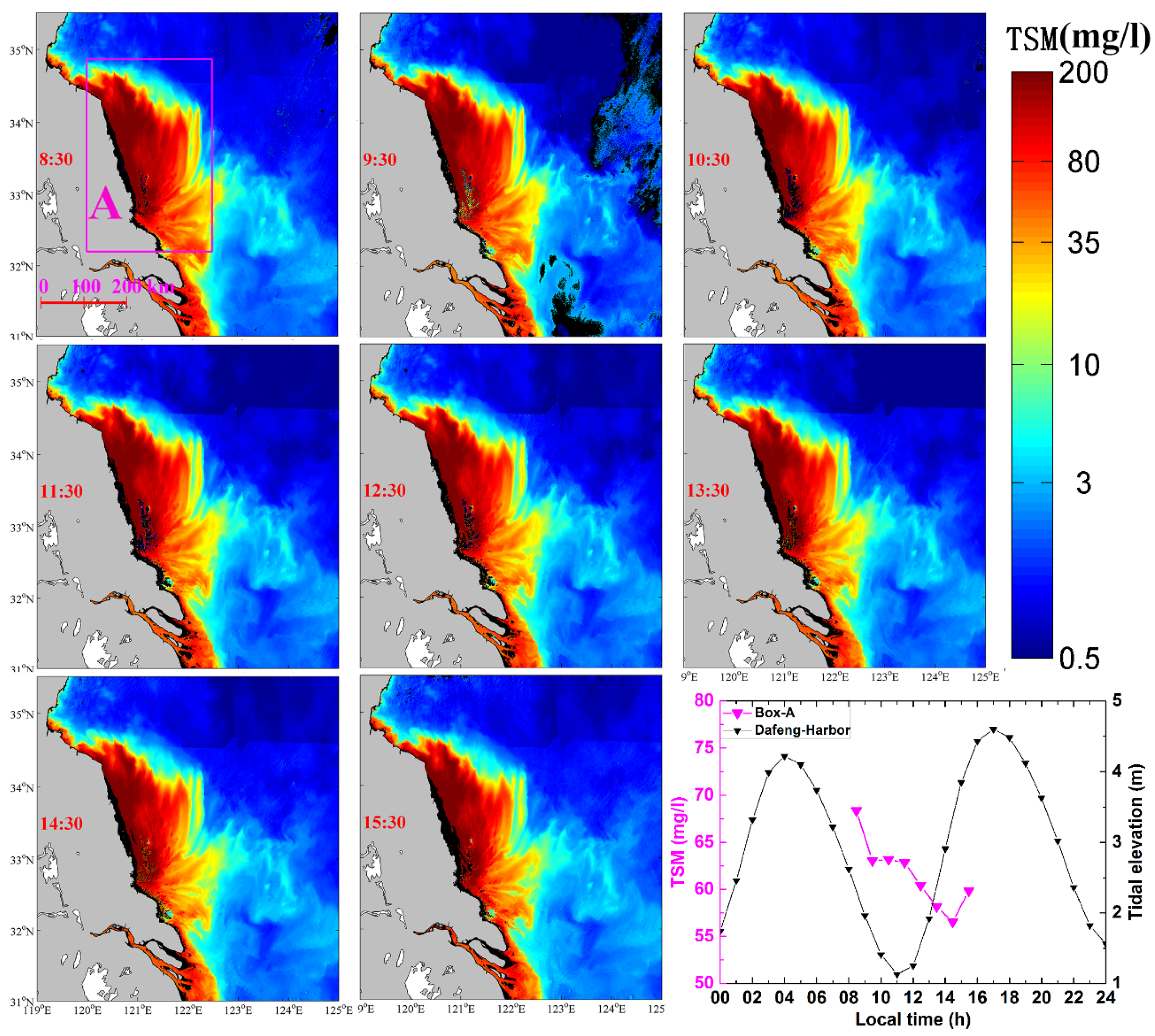
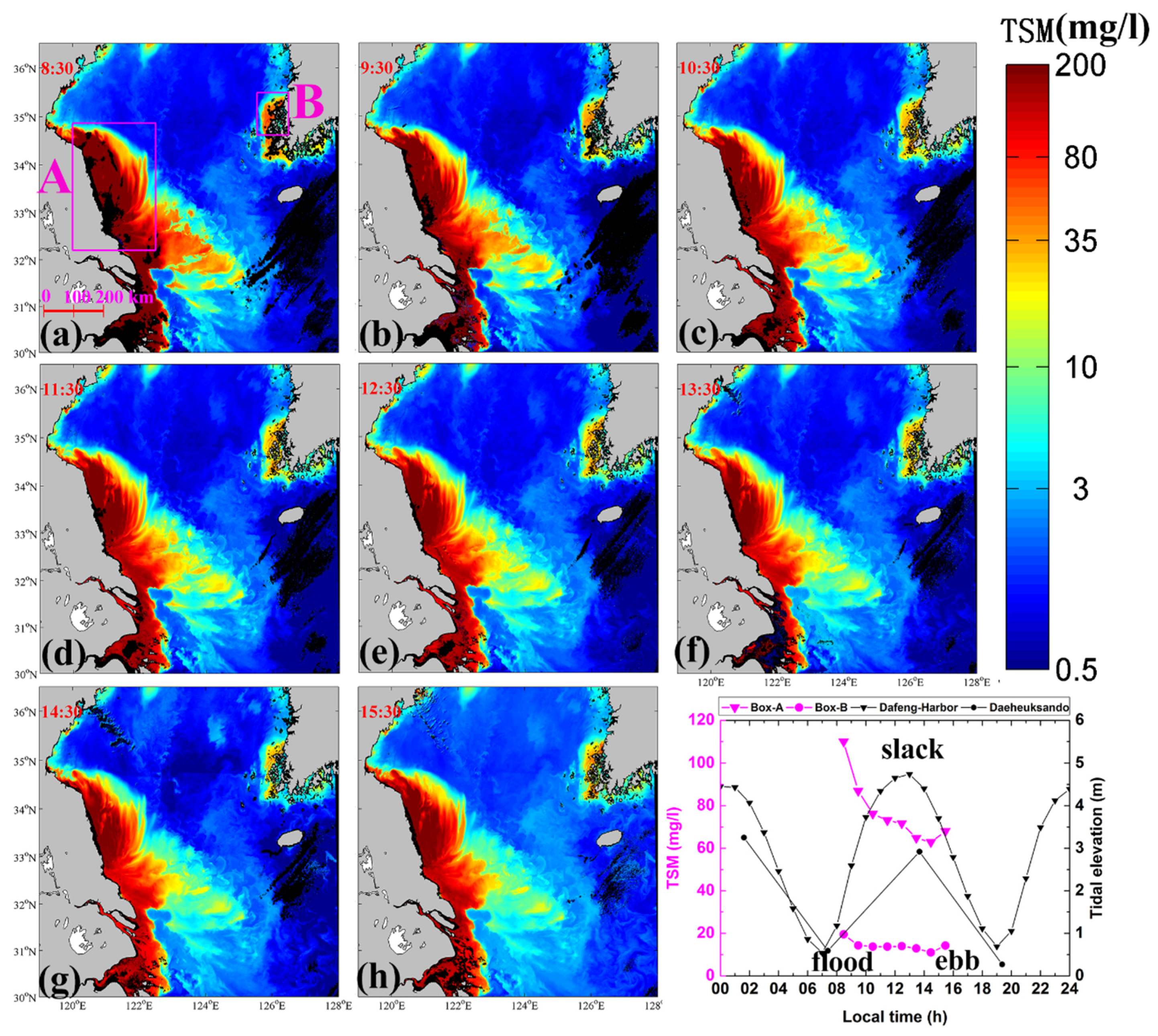
3.1. Diurnal Variability of the GOCI-Derived Total Suspended Matter

Figure 2 shows the GOCI-derived hourly TSM distribution in the YS and ECS. There was a distinct diurnal variability in the coastal waters. In general, high TSM (greater than 10 mg/L) mainly occurred in water depths shallower than 50 m in NJSW and SKCW where the TSM gradually decreased in flood and slack tide, and then increased about one hour later. In contrast, much lower TSM occurred in the central YS and the eastern ECS with water depth generally deeper than 60 m, where no significant TSM diurnal variation (larger than 3 mg/L) was noted. In order to examine the relationship between tide and TSM variations, the hourly averaged TSM in NJSW and SKCW were calculated and shown in the bottom-right plot of Figure 2. The mean TSM in NJSW (Box A) decreased from 109.93 to 71.64 mg/L during the flood tide and then increased around one hour after the slack water. In SKCW, the fluctuation amplitude of the mean TSM was much lower than that of NJSW. The mean TSM in SKCW (Box B) firstly decreased from 19.54 to 13.77 mg/L, and remained steady during flood tide. The second TSM reduction was observed in the slack tide, and reached its minimum value (about 10.97 mg/L) about one hour later. After that, the TSM increased in the ebb tide.
Figure 2. Hourly GOCI-derived TSM images on 5 April 2011. The black areas are the regions masked by the atmospheric correct processing in GDPS due to the cloud coverage (in the shelf) or very high reflectance at the near infrared wavelength (along the coasts). The corresponding observation time (GMT+8) is labeled in each image. The averaged TSM in NJSW (Box A) and SKCW (Box B) (Figure 2a) and the tidal elevation from tide tables are shown in the bottom-right plot.
Remotesensing 08 00147 g002

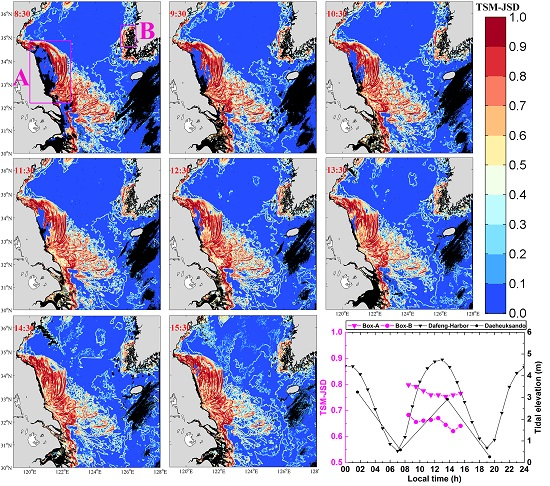
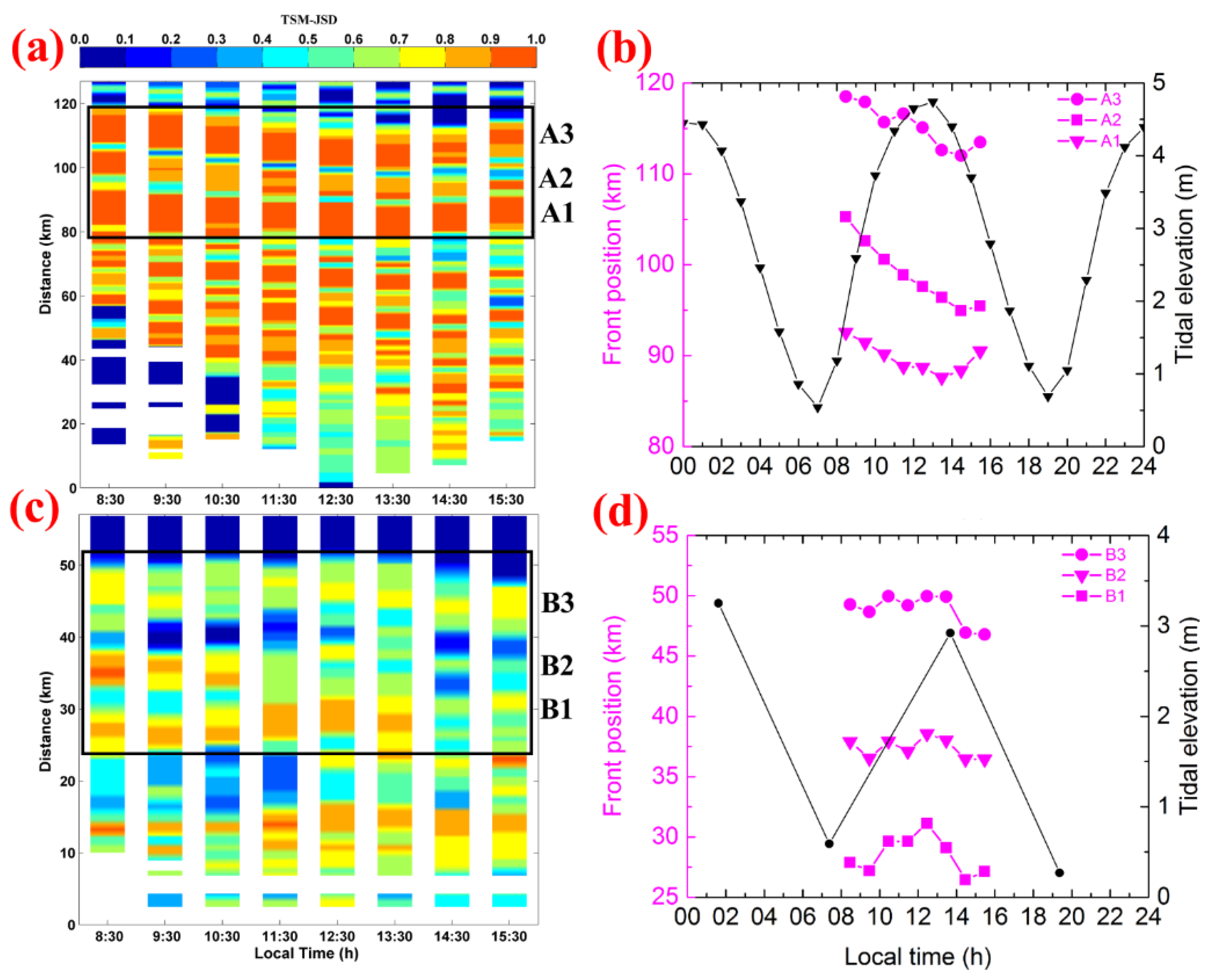
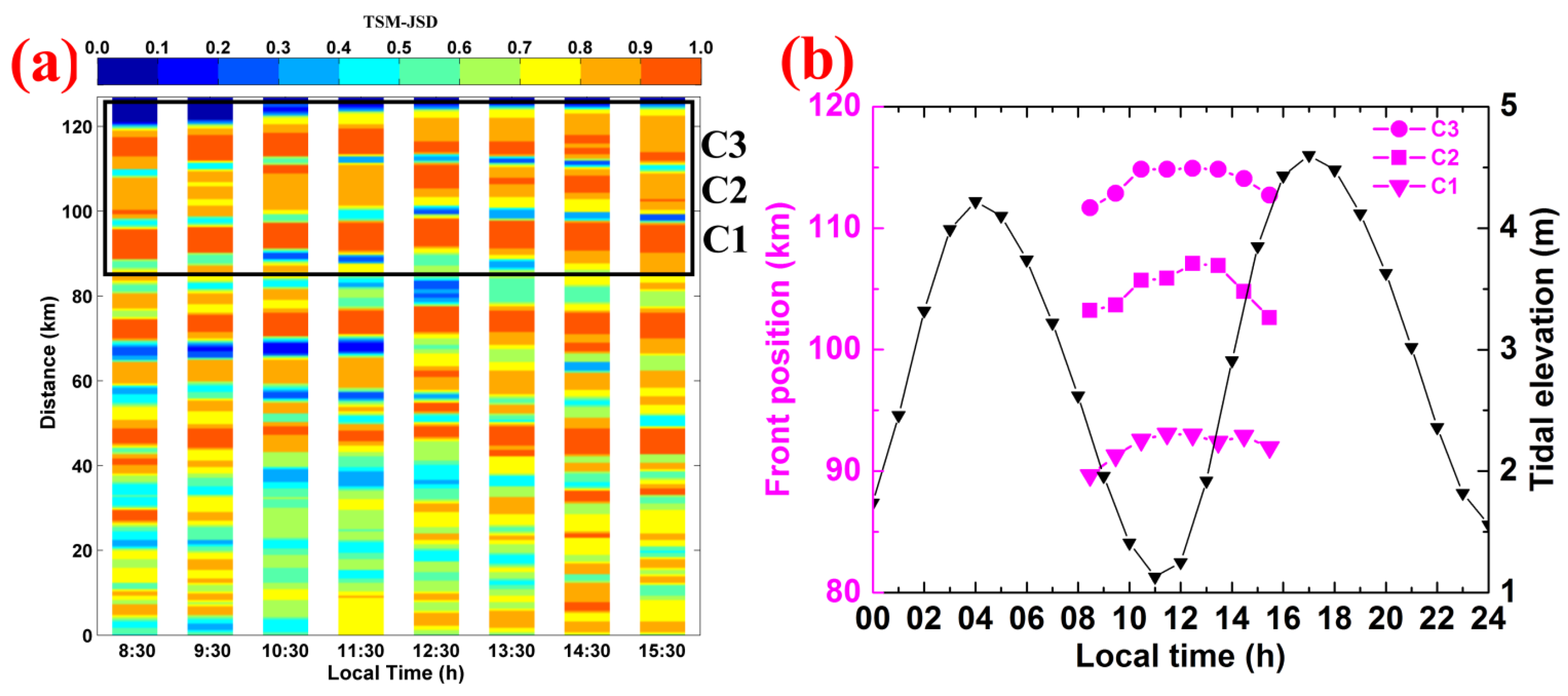
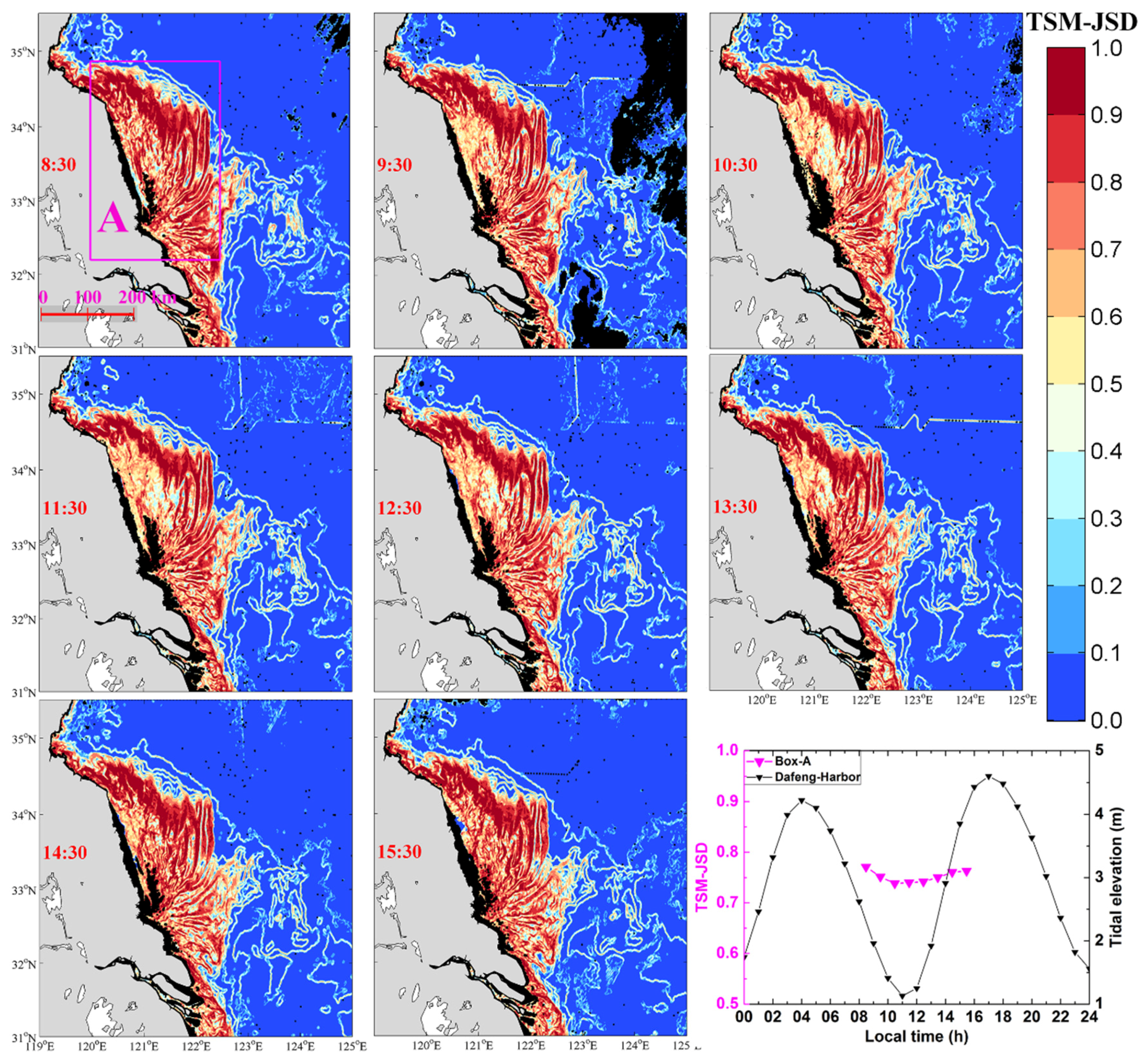
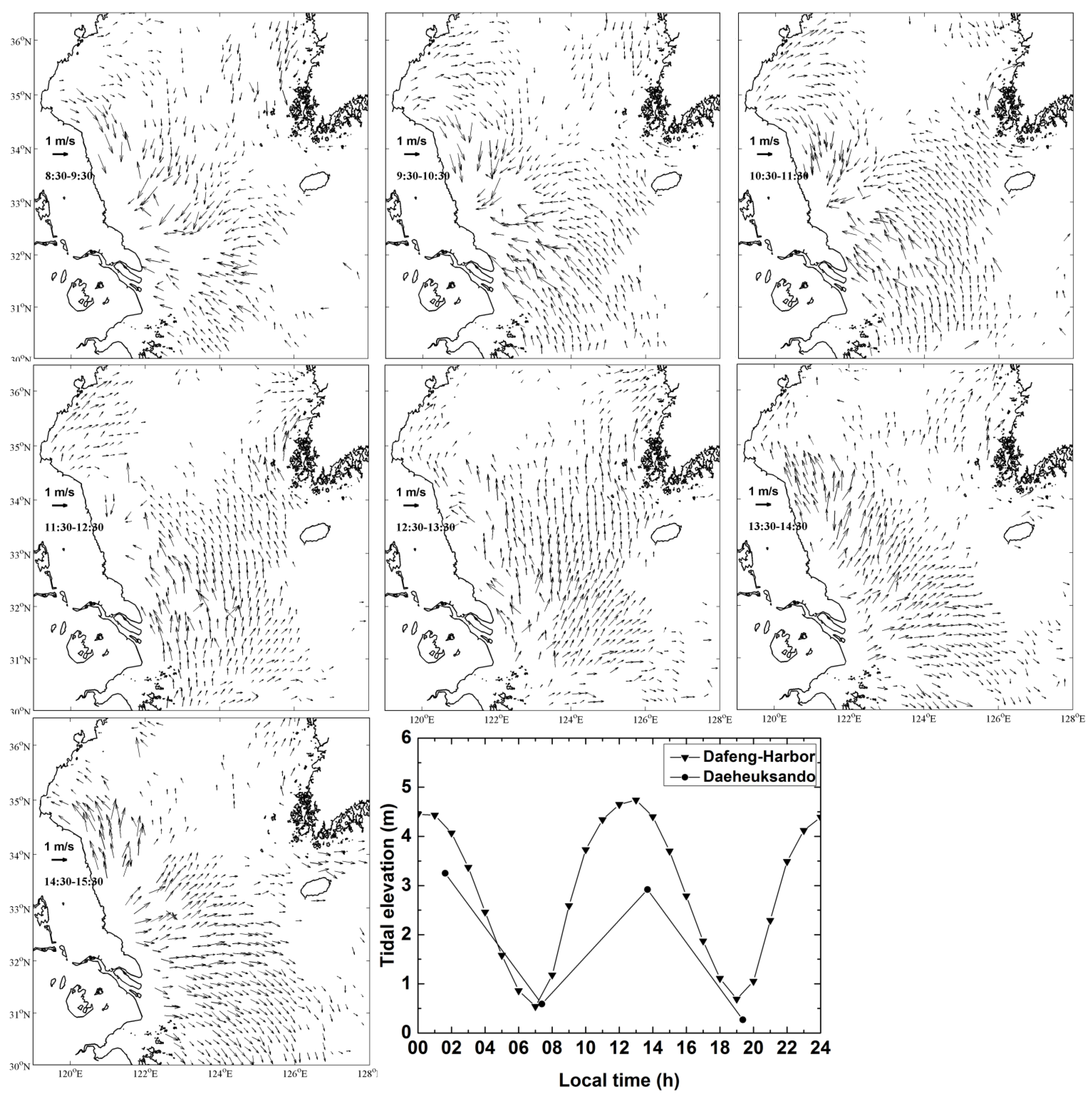
3.2. Diurnal Dynamics of Turbidity Fronts

Figure 3 shows the hourly distributions of TSM–JSD. The turbidity fronts mainly occurred over the shallow shelf water of the YS and ECS where there was distinct TSM variability. The hourly varying tendencies of the turbidity fronts were evident and generally consistent with those of TSM. In NJSW, the front variations exhibited shoreward and seaward fluctuation within depths shallower than about 30 m; the offshore extension could be up to 270 km away from the Chinese coast. In SKCW, the front fluctuation occurred along the Korean coast and was principally confined to shallow waters with depth less than 50 m. The offshore extension of turbidity front could be up to 52 km from the Korean coast, which was much closer to the coast as compared with that in NJSW.
The front intensity gradually weakened during flood tide and the early ebb tide, and became stronger about 1 hour after slack water. The hourly series of the mean front intensity (TSM–JSD) in NJSW and SKCW were calculated and shown in the bottom-right subplot. The mean front intensity in NJSW (Box A) decreased from about 0.80 to 0.75 during the flood tide, and then increased around one hour after the slack water. In SKCW (Box B), the mean front intensity ranged from 0.68 to 0.62, with an average value of 0.66. It was obvious that the front intensity were much stronger in NJSW (about 0.77) than in SKCW (about 0.66). Within the observation time, the varying tendency of the mean front intensity in SKCW was similar to that in NJSW, showing that front intensity became decayed during the early flood tide and then strengthened about one hour after slack tide, but a slight difference during the late flood tide and slack water.
Figure 3. Hourly front patterns derived from GOCI TSM images on 5 April 2011. The black areas are the regions masked by the atmospheric correct processing in GDPS due to the cloud coverage (in the shelf) or very high reflectance at the near infrared wavelength (along the coasts). The corresponding observation time (GMT+8) is labeled in each image. The averaged TSM–JSD in NJSW (Box A) and SKCW (Box B) (in the subplot at 8:30) and tidal elevation from tide tables are shown in the bottom-right plot.
Remotesensing 08 00147 g003
To quantitatively analyze diurnal variations of intensity and displacement of the turbidity fronts, two cross-front transects (shown in Figure 1) were selected in NJSW and SKCW, where diverse intensity of turbidity fronts was frequently detected. Figure 4a,c showed the temporal variations of the TSM–JSD at each GOCI observing time along the transects A and B, respectively. It was obvious that the front intensity and fluctuation, along the transect A, varied more significantly than those along the transect B. The mean TSM–JSD along the whole transect A gradually decreased from about 0.85 at 8:30 to 0.74 at 12:30, and then slightly increased. The maximum and minimum values (0.71 and 0.63) of the mean TSM–JSD along the whole transect B occurred at 11:30 and 14:30, respectively. Moreover, the number of strong fronts with TSM–JSD greater than 0.7 along the transect A is larger than it along the transect B.
Three offshore front peaks at each transect were chosen to quantitatively investigate their displacements (A1, A2, and A3 in Figure 4a, and B1, B2, and B3 in Figure 4c). Figure 4b,d showed the offshore distances of each peak at eight GOCI observing times. The offshore distances along the transect A ranged from 87.6 to 92.6 km for A1, from 95.0 to 105.3 km for A2, and from 112.0 to 118.5 km for A3, respectively. The mean speed of horizontal displacement of the A1, A2 and A3 was about 1.4 km/h. During the flood tide, the positions of the A1, A2, and A3 moved shoreward. As the tidal flow direction was reversed from flood to ebb tide, the front positions gradually advected offshore, similar to the general patterns of front extensions shown in Figure 3. During the eight times of GOCI observations on 5 April 2011, the maximum displacements for A1, A2, and A3 were approximately 5.0, 10.3, and 6.5 km, respectively, with averaged value of about 7.3 km. Along the transect B, the offshore distances ranged from 26.4 to 31.1 km for B1, from 36.5 to 38.6 km for B2, and from 46.8 to 50.0 km for B3, respectively. The B2 and B3 were relatively stable during the flood tide, and rapidly shrank shoreward during the slack tide. The maximum displacements for the B1, B2, and B3 over the GOCI eight times of observations on 5 April 2011 were about 4.7, 2.1, and 3.2 km, respectively, with the averaged value of 3.3 km. The mean speed of horizontal displacement of the B1, B2 and B3 was around 1.1 km/h. The diurnal variability of turbidity fronts in NJSW was greater than it in SKCW.
Figure 4. (a) temporal variability of the TSM–JSD along the transect A in NJSW (Figure 1) with three relatively strong fronts marked as A1, A2, and A3; (b) hourly variability of the position of fronts A1, A2, and A3, overlaid with tide height at the corresponding gauge station A; (c) temporal variability of the TSM–JSD along the transect B in SKCW (Figure 1) with three relatively strong fronts marked as B1, B2, and B3; (d) Hourly variability of the position of fronts B1, B2, and B3, overlaid with tide height at the corresponding gauge station B.
Remotesensing 08 00147 g004

3.3. Variability of Turbidity Fronts at Different Tidal Phases

In order to compare with relatively large variability of turbidity fronts during spring tide in NJSW, hourly images obtained on 12 May 2015 during neap tide were analyzed. Figure 5 and Figure 6 suggest that similar diurnal variations of TSM and turbidity fronts could be also successfully observed at different tidal phases. The shoreward and seaward oscillations during flood-ebb cycle tide were very similar to those obtained on 5 April 2011 (Figure 2 and Figure 3). The variability of TSM and turbidity fronts during neap tide was less significant than that during spring tide. The relatively high TSM (>10 mg/L) and turbidity fronts were mainly confined to shallow waters with depth less than 20 m (Figure 5 and Figure 6). For the hourly series of front intensity averaged in Box-A (bottom-right subplot shown in Figure 6), they gradually weakened in the late ebb tide, and then strengthened after the reversal of tidal current. The mean front intensity ranged from 0.74 to 0.77, with an average value of 0.75. Overall, the front intensity during neap tide was slightly lower than that during spring tide (about 0.77).
Similarly, the cross-front transect A was selected to quantitatively analyze the diurnal variations of intensity and displacement of the turbidity fronts during the neap tide. Figure 7a showed the temporal variations of TSM–JSD along the transect A. The weakest fronts were observed in the late ebb tide (about 10:30). The front intensity increased again with the starting of the flood tide. The mean TSM–JSD for the whole transect A ranged from 0.76 (10:30) to 0.80 (14:30). Overall, the mean front intensity during neap tide (~0.76) was slightly weaker than that during spring tide (~0.79). Meanwhile, three offshore front peaks along transect A (C1, C2 and C3 in Figure 7a) were selected for investigating their diurnal displacements relative to coast. The turbidity front positions moved offshore during ebb tide, and then veered shoreward about one hour after reversal of tidal direction (flood tide) (Figure 7b). The offshore distances ranged from 89.7 to 93.1 km for C1, from 102.6 to 107.0 km for C2, and from 111.7 to 114.9 km for C3, respectively. The maximum displacements for the C1, C2, and C3 fronts were approximately 3.4, 4.4, and 3.2 km during the GOCI eight times of observation, respectively, with an average value of about 3.7 km (Figure 7b). The mean displacement speed of C1, C2 and C3 was about 0.9 km/h, which was much slower than that during spring tide (~1.4 km/h). The above results showed that the frontal intensity and displacement during neap tide oscillated weaker in comparison with that during spring tide.
Figure 5. Hourly GOCI-derived TSM images on 12 May 2015. The black areas are the regions masked by the atmospheric correct processing in GDPS due to the cloud coverage (in the shelf) or very high reflectance at the near infrared wavelength (along the coasts). The corresponding observation time (GMT+8) is labeled in each image. The averaged TSM in NJSW (Box A in subplot at 8:30) and the tidal elevation from tide tables are shown in the bottom-right plot.
Remotesensing 08 00147 g005
Figure 6. Hourly front patterns derived from GOCI TSM images on 12 May 2015. The black areas are the regions masked by the atmospheric correct processing in GDPS due to the cloud coverage (in the shelf) or very high reflectance at the near infrared wavelength (along the coasts). The corresponding observation time (GMT+8) is labeled in each image. The averaged TSM–JSD in NJSW (Box A in subplot at 8:30) and tidal elevation from tide tables at the tide gauge stations is shown in the bottom-right plot.
Remotesensing 08 00147 g006
Figure 7. (a) temporal variability of the TSM–JSD along the transect A in NJSW with three relatively strong fronts marked as C1, C2, and C3. (b) hourly variability of the position of fronts C1, C2, and C3, overlaid with tide height at the corresponding gauge station A.
Remotesensing 08 00147 g007

4. Discussion

There have been few reports about frontal displacement over tidal cycle, not to mention hourly variations. In the United Kingdom shelf seas, Simpson and Bowers [29] found that a spring-neap frontal displacement was about 4 km, and that eddy instabilities induced the front perturbation and about 7 km variability in frontal displacement. In the Gulf of California, Paden et al. [30] found that the tidal front moved approximately 10–15 km under the influence of a spring-neap tide. In the Clyde Sea, Kasai et al. [31] observed that the tidal currents over one tidal cycle could induce 3–5 km displacement of the thermohaline front. In addition, Hopkins and Polton [32] found that the movement of the Liverpool Bay thermohaline front ranged from 5 km to 35 km driven by spring-neap variability in tidal mixing, and the semidiurnal superimposed flood-ebb tidal currents made 5–10 km contributions to the movement. Pisoni, et al. [33] showed that position oscillations of about 10 km and 15 km amplitude occurred in the San Matías and Valdés fronts, respectively, in response to the spring-neap transition. In this study, the horizontal displacement of turbidity fronts oscillated approximately 2.1–10.3 km, which are of the same order of magnitude as previous reports of tidal front displacements.
Tidal characteristics play a significant role in frontal intensity and persistence [28]. The ubiquitous tide is one of the most significant physical processes in the YS and ECS, which are dominated by semidiurnal tidal currents [60]. About 9% of global M2 tidal dissipation is contributed by the shallow coastal China seas through bottom friction dissipation [61,62], where the strong tidal currents can reach up to 1 m/s [62]. To explore the coupling between ocean currents and high-frequency frontal variability, the hourly sea surface currents were estimated from successive GOCI-derived TSM images (shown in Figure 8). The GOCI-derived surface currents are the total currents including tidal currents and residual currents. It is obvious that the diurnal variability of surface current magnitude and direction is generally consistent with that of tidal height, suggesting that the surface currents are principally determined by tidal currents rather than residual currents. Near the transect A in NJSW, the surface currents gradually rotate clockwise and tend to orient in the onshore direction, which is in close agreement with previous studies [63,64]. During the flood tide, the shoreward currents bring clear outer shelf water and reduce the TSM concentration in the inner shelf (Figure 2), thereby inducing the shoreward progression of front positions (Figure 3 and Figure 4a,b). When the direction of flow velocity reverses from flood to ebb at around 13:00, the offshore surface currents move the frontal position seaward. Unlike in NJSW, the sea surface currents in SKCW generally oscillate along the Korean coast, which support the findings of Lie et al. [65] based on multi-year satellite-tracked drifter trajectories. In contrast to the transect A in NJSW, the surface current directions are almost perpendicular to the transect B in SKCW, which might be responsible for the relatively weak oscillation of the frontal positions compared with those at the transect A (Figure 4). These results indicate that the processes of flood-ebb advection rather than vertical mixing appear to be more important in frontal displacement variability, which is similar to observations in the Gulf of California where the variability of frontal displacement was observed over the spring-neap tidal cycle [30].
The diurnal variations in TSM are frequently observed in other regions, for example, in the Bohai and ECS Seas [37,46], in the Southern North Sea [66,67]. The tide-induced turbulent mixing and wave-current interaction in the inner shelf region of YS are capable of stirring a large amount of sediment to the surface layer, resulting in TSM variations [46,49,68], which could further influence turbidity frontal patterns through sediment resuspension and deposition. During the ebb-flood transition or slack water, the reduced bottom shear stress weakens the vertical sediment resuspension, which might induce high-frequency seaward and shoreward oscillation at the B1 front (Figure 4d) and make it mix more easily with its neighboring fronts because of the front position close to the coast. The onshore–offshore fluctuation of front displacements on an hourly scale might not be induced by winds and the suspended sediments transport from surrounding coastal regions, since the residual currents (coastal currents) are along the coasts [69], and winds showed less significant variation for the two days (not shown). Instead, the dominant tidal currents, when combined with local bathymetry effects, are more likely to provide a mechanism for the variability of the turbidity fronts in both the NJSW and SKCW coastal waters.
Figure 8. Hourly sea surface currents derived from GOCI TSM images on 5 April 2011. The corresponding observation time (GMT+8) is labeled in each image. The tidal elevation from tide tables at the tide gauge stations is shown in the bottom-right plot.
Remotesensing 08 00147 g008
Oceanic fronts, conventionally known as “hot spots” of marine life, have a significant impact on the marine ecosystem [16,17,28,70,71]. They are probably responsible for enhanced nutrients and the light exposure induced by front dynamics [1,72]. Scales et al. [71] reviewed current understanding of association between marine vertebrates and multiple scale fronts, and highlighted the ecological importance of frontal zones in identifying pelagic foraging hotspots, understanding of pelagic ecosystem function and predicting the taxa of bioaggregation in different oceanographic regions. Unlike thermal fronts, turbidity fronts are the boundary between two water masses with different turbidity, such as terrestrial-dominated coastal water and clear open ocean water. Wang, et al. [68] argued that low TSM could enhance the penetration of photosynthetically available radiation in NJSW, and, therefore, significantly increase local growth of phytoplankton. Byun et al. [73] also suggested that enhanced sediment resuspension can inhibit the development of phytoplankton blooms in the tidally turbid coastal waters of southwest Korea. In the coastal frontal regions with high TSM (Figure 2, Figure 3, Figure 5 and Figure 6), it is difficult to observe the spawning and overwintering grounds of major commercial fisheries [16].

5. Conclusions

Using the entropy-based front detection technique, this study explores the capacity of applying the world’s first Geostationary Ocean Color Imager (GOCI) with high spatiotemporal resolution (500 m and one hour) to analyze the diurnal variability of turbidity fronts and their displacements. The horizontal displacements of turbidity fronts oscillated approximately 3.2–10.3 and 2.1–4.7 km in NJSW and SKCW, respectively. Moreover, the comparison at different tidal phases in NJSW suggests that the turbidity fronts oscillates more significantly during spring tide than neap tide. In addition, this research highlighted the feasibility of using the geostationary ocean color remote sensing combined with the entropy-based front detection technique to monitor the diurnal variability of turbidity fronts. Because water turbidity rather than SST can provide more direct indication of terrestrial material transportation [9], the GOCI-derived turbidity front structure can be used to identify the extending of river plume, such as the Changjiang River plume. In addition, the GOCI-derived diurnal displacement of turbidity front is helpful for studying the association between marine frontal zones and the pelagic richness and diversity (e.g., phytoplankton bloom, foraging and migration), and for exploring the biophysical interaction induced by multi-scale physical processes in further studies.
Moreover, based on GOCI-derived TSM images, the maximum cross-correlation (MCC) technique was implemented to estimate the hourly sea surface currents for exploring the coupling between ocean currents and high-frequency frontal variability. The results suggest that the onshore–offshore and alongshore oscillations of tide-dominated currents in NJSW and SKCW may induce the discrepancy of frontal variability, and that the ocean currents, when combined with local bathymetry effects, are more probably responsible for the high-frequency variability of the turbidity fronts through influencing sediment resuspension and deposition. The study shows that the GOCI satellite has a great potential in monitoring the dynamics of fine-scale and highly variable fronts, which will benefit studies of the coupling of bio-physical processes.

Acknowledgments

GOCI Level-1B data were provided by the Korea Institute of Ocean Science and Technology (KIOST). The authors would like to thank WooChang Choi for data acquirement, and Teruhisa Shimada for algorithm support. This study was supported by the National High Technology and Development Program of China (grant #2014AA123301), the National Basic Research Program (973 Program) of China (Grant #2015CB954002), the Public Science and Technology Research Fund Projects for Ocean Research (grant #201505003), the National Natural Science Foundation of China (grants #41322039, #41321004, #41271378, and #41406202), and the National Program on Global Change and Air-Sea Interaction of China (grants #GASI-03-03-01-01, #GASI-02-SCS-YGST01, #GASI-02-PAC-YGST01, and #GASI-02-IND-YGST01).

Author Contributions

Zifeng Hu, Delu Pan and Xianqiang He conceived the study. Zifeng Hu processed the GOCI data. Zifeng Hu, Xianqiang He, and Yan Bai wrote the manuscript.

Conflicts of Interest

The authors declare no conflict of interest.

References

  1. Taylor, J.R.; Ferrari, R. Ocean fronts trigger high latitude phytoplankton blooms. Geophys. Res. Lett. 2011, 38. [Google Scholar] [CrossRef]
  2. Ullman, D.S.; Cornillon, P.C. Satellite-derived sea surface temperature fronts on the continental shelf off the northeast U.S. coast. J. Geophys. Res. 1999, 104, 23459–23478. [Google Scholar] [CrossRef]
  3. Chen, D.; Liu, W.T.; Tang, W.Q.; Wang, Z.R. Air-sea interaction at an oceanic front: Implications for frontogenesis and primary production. Geophys. Res. Lett. 2003, 30. [Google Scholar] [CrossRef]
  4. Belkin, I.; Cornillon, P. SST fronts of the Pacific coastal and marginal seas. Pacific Oceanogr. 2003, 1, 90–113. [Google Scholar]
  5. Belkin, I.M.; O’Reilly, J.E. An algorithm for oceanic front detection in chlorophyll and SST satellite imagery. J. Mar. Syst. 2009, 78, 319–326. [Google Scholar] [CrossRef]
  6. Dzwonkowski, B.; Yan, X.-H. Tracking of a Chesapeake Bay estuarine outflow plume with satellite-based ocean color data. Cont. Shelf Res. 2005, 25, 1942–1958. [Google Scholar] [CrossRef]
  7. Miller, P. Multi-spectral front maps for automatic detection of ocean colour features from SeaWiFS. Int. J. Remote Sens. 2004, 25, 1437–1442. [Google Scholar] [CrossRef]
  8. Miller, P. Composite front maps for improved visibility of dynamic sea-surface features on cloudy SeaWiFS and AVHRR data. J. Mar. Syst. 2009, 78, 327–336. [Google Scholar] [CrossRef]
  9. Miller, P.I.; Xu, W.; Carruthers, M. Seasonal shelf-sea front mapping using satellite ocean colour and temperature to support development of a marine protected area network. Deep-Sea Res. Part II-Top. Stud. Oceanogr. 2015, 119, 3–19. [Google Scholar] [CrossRef]
  10. Saldías, G.S.; Sobarzo, M.; Largier, J.; Moffat, C.; Letelier, R. Seasonal variability of turbid river plumes off central Chile based on high-resolution MODIS imagery. Remote Sens. Environ. 2012, 123, 220–233. [Google Scholar] [CrossRef]
  11. Shimada, T.; Sakaida, F.; Kawamura, H.; Okumura, T. Application of an edge detection method to satellite images for distinguishing sea surface temperature fronts near the Japanese coast. Remote Sens. Environ. 2005, 98, 21–34. [Google Scholar] [CrossRef]
  12. Stegmann, P.M.; Ullman, D.S. Variability in chlorophyll and sea surface temperature fronts in the Long Island Sound outflow region from satellite observations. J. Geophys. Res. 2004, 109, S03. [Google Scholar] [CrossRef]
  13. Bai, Y.; He, X.; Pan, D.; Chen, C.-T.A.; Kang, Y.; Chen, X.; Cai, W.-J. Summertime Changjiang River plume variation during 1998–2010. J. Geophys. Res. 2014, 119, 6238–6257. [Google Scholar] [CrossRef]
  14. He, S.; Huang, D.; Zeng, D. Double SST fronts observed from MODIS data in the East China Sea off the Zhejiang-Fujian coast, China. J. Mar. Syst. 2016, 154, 93–102. [Google Scholar] [CrossRef]
  15. Hickox, R.; Belkin, I.; Cornillon, P.; Shan, Z. Climatology and seasonal variability of ocean fronts in the East China, Yellow and Bohai Seas from satellite SST data. Geophys. Res. Lett. 2000, 27, 2945–2948. [Google Scholar] [CrossRef]
  16. Huang, D.; Zhang, T.; Zhou, F. Sea-surface temperature fronts in the Yellow and East China Seas from TRMM microwave imager data. Deep-Sea Res. Part II-Top. Stud. Oceanogr. 2010, 57, 1017–1024. [Google Scholar] [CrossRef]
  17. Chen, C.T.A. Chemical and physical fronts in the Bohai, Yellow and East China Seas. J. Mar. Syst. 2009, 78, 394–410. [Google Scholar] [CrossRef]
  18. Bontempi, P.S.; Yoder, J.A. Spatial variability in SeaWiFS imagery of the South Atlantic bight as evidenced by gradients (fronts) in chlorophyll a and water-leaving radiance. Deep-Sea Res. Part II-Top. Stud. Oceanogr. 2004, 51, 1019–1032. [Google Scholar] [CrossRef]
  19. Bai, Y.; Pan, D.; Cai, W.-J.; He, X.; Wang, D.; Tao, B.; Zhu, Q. Remote sensing of salinity from satellite-derived CDOM in the Changjiang River dominated East China Sea. J. Geophys. Res. 2013, 118, 227–243. [Google Scholar] [CrossRef]
  20. Lihan, T.; Saitoh, S.-I.; Iida, T.; Hirawake, T.; Iida, K. Satellite-measured temporal and spatial variability of the Tokachi River plume. Estuar. Coast. Shelf Sci. 2008, 78, 237–249. [Google Scholar] [CrossRef]
  21. Jabbar, A.; Lihan, T.; Mustapha, M.; Rahman, Z.; Rahim, S. Variability of river plume signature determined using satellite images. J. Appl. Sci. 2013, 13, 70–78. [Google Scholar]
  22. Valente, A.S.; da Silva, J.C.B. On the observability of the fortnightly cycle of the Tagus estuary turbid plume using MODIS ocean colour images. J. Mar. Syst. 2009, 75, 131–137. [Google Scholar] [CrossRef]
  23. Mendes, R.; Vaz, N.; Fernández-Nóvoa, D.; da Silva, J.C.B.; deCastro, M.; Gómez-Gesteira, M.; Dias, J.M. Observation of a turbid plume using MODIS imagery: The case of Douro estuary (Portugal). Remote Sens. Environ. 2014, 154, 127–138. [Google Scholar] [CrossRef]
  24. Wall, C.C.; Muller-Karger, F.E.; Roffer, M.A.; Hu, C.; Yao, W.; Luther, M.E. Satellite remote sensing of surface oceanic fronts in coastal waters off west–central Florida. Remote Sens. Environ. 2008, 112, 2963–2976. [Google Scholar] [CrossRef]
  25. Miller, P.I.; Read, J.F.; Dale, A.C. Thermal front variability along the North Atlantic current observed using microwave and infrared satellite data. Deep-Sea Res. Part II-Top. Stud. Oceanogr. 2013, 98, 244–256. [Google Scholar] [CrossRef]
  26. Bai, Y.; Huang, T.-H.; He, X.; Wang, S.-L.; Hsin, Y.-C.; Wu, C.-R.; Zhai, W.; Lui, H.-K.; Chen, C.-T.A. Intrusion of the Pearl River plume into the main channel of the Taiwan Strait in summer. J. Sea Res. 2015, 95, 1–15. [Google Scholar] [CrossRef]
  27. He, X.; Bai, Y.; Chen, C.T.A.; Hsin, Y.C.; Wu, C.R.; Zhai, W.; Liu, Z.; Gong, F. Satellite views of the episodic terrestrial material transport to the southern Okinawa Trough driven by typhoon. J. Geophys. Res. 2014, 119, 4490–4504. [Google Scholar] [CrossRef]
  28. Belkin, I.M.; Cornillon, P.C.; Sherman, K. Fronts in large marine ecosystems. Prog. Oceanogr. 2009, 81, 223–236. [Google Scholar] [CrossRef]
  29. Simpson, J.H.; Bowers, D. Models of stratification and frontal movement in shelf seas. Deep-Sea Res. A: Oceanogr. Res. Pap. 1981, 28, 727–738. [Google Scholar] [CrossRef]
  30. Paden, C.A.; Abbott, M.R.; Winant, C.D. Tidal and atmospheric forcing of the upper ocean in the Gulf of California: 1. Sea surface temperature variability. J. Geophys. Res. 1991, 96, 18337–18359. [Google Scholar] [CrossRef]
  31. Kasai, A.; Rippeth, T.P.; Simpson, J.H. Density and flow structure in the Clyde Sea front. Cont. Shelf Res. 1999, 19, 1833–1848. [Google Scholar] [CrossRef]
  32. Hopkins, J.; Polton, J. Scales and structure of frontal adjustment and freshwater export in a region of freshwater influence. Ocean Dyn. 2012, 62, 45–62. [Google Scholar] [CrossRef] [Green Version]
  33. Pisoni, J.P.; Rivas, A.L.; Piola, A.R. On the variability of tidal fronts on a macrotidal continental shelf, Northern Patagonia, Argentina. Deep-Sea Res. Part II-Top. Stud. Oceanogr. 2015, 119, 61–68. [Google Scholar] [CrossRef]
  34. Ryu, J.H.; Choi, J.K.; Eom, J.; Ahn, J.H. Temporal variation in Korean coastal waters using Geostationary Ocean Color Imager. J. Coast. Res. 2011, 64, 1731–1735. [Google Scholar]
  35. He, X.Q.; Bai, Y.; Pan, D.L.; Huang, N.L.; Dong, X.; Chen, J.S.; Chen, C.-T.A.; Cui, Q.F. Using geostationary satellite ocean color data to map the diurnal dynamics of suspended particulate matter in coastal waters. Remote Sens. Environ. 2013, 133, 225–239. [Google Scholar] [CrossRef]
  36. Lou, X.; Hu, C. Diurnal changes of a harmful algal bloom in the East China Cea: Observations from GOCI. Remote Sens. Environ. 2014, 140, 562–572. [Google Scholar] [CrossRef]
  37. Yang, H.; Choi, J.-K.; Park, Y.-J.; Han, H.-J.; Ryu, J.-H. Application of the Geostationary Ocean Color Imager (GOCI) to estimates of ocean surface currents. J. Geophys. Res. 2014, 119, 3988–4000. [Google Scholar] [CrossRef]
  38. Choi, J.K.; Park, Y.J.; Ahn, J.H.; Lim, H.S.; Eom, J.; Ryu, J.H. GOCI, the world's first geostationary ocean color observation satellite, for the monitoring of temporal variability in coastal water turbidity. J. Geophys. Res. 2012, 117, C9. [Google Scholar] [CrossRef]
  39. Cayula, J.-F.; Cornillon, P. Edge detection algorithm for SST images. J. Atmos. Ocean. Technol. 1992, 9, 67–80. [Google Scholar] [CrossRef]
  40. Cayula, J.-F.; Cornillon, P. Multi-image edge detection for SST images. J. Atmos. Ocean. Technol. 1995, 12, 821–829. [Google Scholar] [CrossRef]
  41. Lan, K.W.; Kawamura, H.; Lee, M.A.; Chang, Y.; Chan, J.W.; Liao, C.H. Summertime sea surface temperature fronts associated with upwelling around the Taiwan Bank. Cont. Shelf Res. 2009, 29, 903–910. [Google Scholar] [CrossRef]
  42. Chang, Y.; Shimada, T.; Lee, M.A.; Lu, H.J.; Sakaida, F.; Kawamura, H. Wintertime sea surface temperature fronts in the Taiwan Strait. Geophys. Res. Lett. 2006, 33. [Google Scholar] [CrossRef]
  43. Chang, Y.; Shieh, W.-J.; Lee, M.-A.; Chan, J.-W.; Lan, K.-W.; Weng, J.-S. Fine-scale sea surface temperature fronts in wintertime in the northern South China Sea. Int. J. Remote Sens. 2010, 31, 4807–4818. [Google Scholar] [CrossRef]
  44. Qiu, C.H.; Kawamura, H. Study on SST front disappearance in the subtropical North Pacific using microwave SSTs. J. Oceanogr. 2012, 68, 417–426. [Google Scholar] [CrossRef]
  45. Min, J.-E.; Choi, J.-K.; Yang, H.; Lee, S.; Ryu, J.-H. Monitoring changes in suspended sediment concentration on the southwestern coast of Korea. J. Coast. Res. 2014, 70, 133–138. [Google Scholar] [CrossRef]
  46. Son, S.; Kim, Y.H.; Kwon, J.I.; Kim, H.C.; Park, K.S. Characterization of spatial and temporal variation of suspended sediments in the Yellow and East China Seas using satellite ocean color data. GISci. Remote Sens. 2014, 51, 212–226. [Google Scholar] [CrossRef]
  47. Zhang, C.K.; Chen, J.; Lin, K.; Ding, X.R.; Yuan, R.H.; Kang, Y.Y. Spatial layout of reclamation of coastal tidal flats in Jiangsu Province. J. Hohai Univ. 2011, 39, 206–212, (in Chinese with English abstract). [Google Scholar]
  48. Dong, L.X.; Guan, W.B.; Chen, Q.; Li, X.H.; Liu, X.H.; Zeng, X.M. Sediment transport in the Yellow Sea and East China Sea. Estuar. Coast. Shelf Sci. 2011, 93, 248–258. [Google Scholar] [CrossRef]
  49. Bian, C.; Jiang, W.; Quan, Q.; Wang, T.; Greatbatch, R.J.; Li, W. Distributions of suspended sediment concentration in the Yellow Sea and East China Sea based on field surveys during the four seasons of 2011. J. Mar. Syst. 2013, 121–122, 24–35. [Google Scholar] [CrossRef]
  50. Kim, J.-E. Land use management and cultural value of ecosystem services in Southwestern Korean islands. J. Mar. Island Cult. 2013, 2, 49–55. [Google Scholar] [CrossRef]
  51. Byun, D.S.; Wang, X.H.; Holloway, P.E. Tidal characteristic adjustment due to dyke and seawall construction in the Mokpo Coastal Zone, Korea. Coast. Shelf Sci. 2004, 59, 185–196. [Google Scholar] [CrossRef]
  52. Ahn, J.-H.; Park, Y.-J.; Kim, W.; Lee, B.; Oh, I.S. Vicarious calibration of the geostationary ocean color imager. Opt. Express 2015, 23, 23236–23258. [Google Scholar] [CrossRef] [PubMed]
  53. Ahn, J.-H.; Park, Y.-J.; Ryu, J.-H.; Lee, B.; Oh, I.S. Development of atmospheric correction algorithm for Geostationary Ocean Color Imager (GOCI). Ocean Sci. J. 2012, 47, 247–259. [Google Scholar] [CrossRef]
  54. Siswanto, E.; Tang, J.; Yamaguchi, H.; Ahn, Y.-H.; Ishizaka, J.; Yoo, S.; Kim, S.-W.; Kiyomoto, Y.; Yamada, K.; Chiang, C.; et al. Empirical ocean-color algorithms to retrieve chlorophyll-a, total suspended matter, and colored dissolved organic matter absorption coefficient in the Yellow and East China Seas. J. Oceanogr. 2011, 67, 627–650. [Google Scholar] [CrossRef]
  55. Moon, J.-E.; Park, Y.-J.; Ryu, J.-H.; Choi, J.-K.; Ahn, J.-H.; Min, J.-E.; Son, Y.-B.; Lee, S.-J.; Han, H.-J.; Ahn, Y.-H. Initial validation of GOCI water products against in situ data collected around Korean Peninsula for 2010–2011. Ocean Sci. J. 2012, 47, 261–277. [Google Scholar] [CrossRef]
  56. Chang, Y.; Cornillon, P. A comparison of satellite-derived sea surface temperature fronts using two edge detection algorithms. Deep-Sea Res. Part II-Top. Stud. Oceanogr. 2013, 119, 40–47. [Google Scholar] [CrossRef]
  57. Castellanos, P.; Pelegrí, J.L.; Baldwin, D.; Emery, W.J.; Hernández-Guerra, A. Winter and spring surface velocity fields in the Cape Blanc region as deduced with the maximum cross-correlation technique. Int. J. Remote Sens. 2013, 34, 3587–3606. [Google Scholar] [CrossRef]
  58. Yang, H.P.; Arnone, R.; Jolliff, J. Estimating advective near-surface currents from ocean color satellite images. Remote Sens. Environ. 2015, 158, 1–14. [Google Scholar] [CrossRef]
  59. Choi, J.K.; Yang, H.; Han, H.J.; Ryu, J.H.; Park, Y.J. Quantitative estimation of suspended sediment movements in coastal region using GOCI. J. Coast. Res. 2013, 65, 1367–1372. [Google Scholar] [CrossRef]
  60. Song, D.; Wang, X.H.; Zhu, X.; Bao, X. Modeling studies of the far-field effects of tidal flat reclamation on tidal dynamics in the East China Seas. Estuar. Coast. Shelf Sci. 2013, 133, 147–160. [Google Scholar] [CrossRef]
  61. Lefèvre, F.; Le Provost, C.; Lyard, F.H. How can we improve a global ocean tide model at a regional scale? A test on the Yellow Sea and the East China Sea. J. Geophys. Res. 2000, 105, 8707–8725. [Google Scholar] [CrossRef]
  62. Provost, C.L.; Lyard, F. Energetics of the M2 barotropic ocean tides: An estimate of bottom friction dissipation from a hydrodynamic model. Prog. Oceanogr. 1997, 40, 37–52. [Google Scholar] [CrossRef]
  63. Li, M.; Rong, Z.R. Effects of tides on freshwater and volume transports in the Changjiang River plume. J. Geophys. Res. 2012, 117, C6. [Google Scholar] [CrossRef]
  64. Lee, J.C.; Jung, K.T. Application of eddy viscosity closure models for the M2 tide and tidal currents in the Yellow Sea and the East China Sea. Cont. Shelf Res. 1999, 19, 445–475. [Google Scholar] [CrossRef]
  65. Lie, H.-J.; Lee, S.; Cho, C.-H. Computation methods of major tidal currents from satellite-tracked drifter positions, with application to the Yellow and East China Seas. J. Geophys. Res. 2002, 107, 3-1–3-22. [Google Scholar]
  66. Neukermans, G.; Ruddick, K.; Bernard, E.; Ramon, D.; Nechad, B.; Deschamps, P.-Y. Mapping total suspended matter from geostationary satellites: A feasibility study with SEVIRI in the Southern North Sea. Opt. Express 2009, 17, 14029–14052. [Google Scholar] [CrossRef] [PubMed]
  67. Neukermans, G.; Ruddick, K.G.; Greenwood, N. Diurnal variability of turbidity and light attenuation in the Southern North Sea from the SEVIRI geostationary sensor. Remote Sens. Environ. 2012, 124, 564–580. [Google Scholar] [CrossRef]
  68. Wang, X.H.; Qiao, F.; Lu, J.; Gong, F. The turbidity maxima of the northern Jiangsu shoal-water in the Yellow Sea, China. Estuar. Coast. Shelf Sci. 2011, 93, 202–211. [Google Scholar] [CrossRef]
  69. Yuan, D.; Zhu, J.; Li, C.; Hu, D. Cross-shelf circulation in the Yellow and East China Seas indicated by MODIS satellite observations. J. Mar. Syst. 2008, 70, 134–149. [Google Scholar] [CrossRef]
  70. Ning, X.; Liu, Z.; Cai, Y.; Fang, M.; Chai, F. Physicobiological oceanographic remote sensing of the East China Sea: Satellite and in situ observations. J. Geophys. Res. 1998, 103, 21623–21635. [Google Scholar] [CrossRef]
  71. Scales, K.L.; Miller, P.I.; Hawkes, L.A.; Ingram, S.N.; Sims, D.W.; Votier, S.C. On the Front Line: frontal zones as priority at-sea conservation areas for mobile marine vertebrates. J. Appl. Ecol. 2014, 51, 1575–1583. [Google Scholar] [CrossRef]
  72. McClatchie, S.; Cowen, R.; Nieto, K.; Greer, A.; Luo, J.Y.; Guigand, C.; Demer, D.; Griffith, D.; Rudnick, D. Resolution of fine biological structure including small narcomedusae across a front in the Southern California Bight. J. Geophys. Res. 2012, 117, C4. [Google Scholar] [CrossRef]
  73. Byun, D.-S.; Wang, X.H.; Zavatarelli, M.; Cho, Y.-K. Effects of resuspended sediments and vertical mixing on phytoplankton spring bloom dynamics in a tidal estuarine embayment. J. Mar. Syst. 2007, 67, 102–118. [Google Scholar] [CrossRef]

