Accuracy of Reconstruction of the Tree Stem Surface Using Terrestrial Close-Range Photogrammetry

Abstract

Airborne laser scanning (ALS) allows for extensive coverage, but the accuracy of tree detection and form can be limited. Although terrestrial laser scanning (TLS) can improve on ALS accuracy, it is rather expensive and area coverage is limited. Multi-view stereopsis (MVS) techniques combining computer vision and photogrammetry may offer some of the coverage benefits of ALS and the improved accuracy of TLS; MVS combines computer vision research and automatic analysis of digital images from common commercial digital cameras with various algorithms to reconstruct three-dimensional (3D) objects with realistic shape and appearance. Despite the relative accuracy (relative geometrical distortion) of the reconstructions available in the processing software, the absolute accuracy is uncertain and difficult to evaluate. We evaluated the data collected by a common digital camera through the processing software (Agisoft PhotoScan ©) for photogrammetry by comparing those by direct measurement of the 3D magnetic motion tracker. Our analyses indicated that the error is mostly concentrated in the portions of the tree where visibility is lower, i.e., the bottom and upper parts of the stem. For each reference point from the digitizer we determined how many cameras could view this point. With a greater number of cameras we found increasing accuracy of the measured object space point positions (as expected), with a significant positive change in the trend beyond five cameras; when more than five cameras could view this point, the accuracy began to increase more abruptly, but eight cameras or more provided no increases in accuracy. This method allows for the retrieval of larger datasets from the measurements, which could improve the accuracy of estimates of 3D structure of trees at potentially reduced costs.

1. Introduction

In forest biometrics and other related research areas, analysis of three-dimensional (3D) data has gained a great deal of attention during the last decade. The 3D data may be characterized by three primary acquisition methods: (1) by scanned by laser; (2) by magnetic motion tracker, and (3) by photogrammetric reconstruction (stereoscopy). The data can also be divided into so-called surface data and structural data. Surface data are sensed directly from the surface of the three-dimensional object and are relatively easily and quickly displayable. Structural data describe the structure, i.e., the permanent relation of several features [1], of an organism, such as a plant or a tree. Features include common geometric shapes such as cylinders, spheres, and rectangles. The main advantage of structural data is that they describe the parts of a tree more directly, thus it provides an overview of the architecture and appearance of a tree. Estimates of tree biomass are easily quantified based on the length and volumes of individual segments, such as branches, bole, crown, and roots [2,3].

Light detection and ranging (LiDAR) technology allows us to measure terrestrial 3D data, and is widely used for commercial purposes in forest inventories [4,5,6]. Airborne LiDAR tends to slightly underestimate field-measured estimates in the case of dense forest stands because of its poor ability to penetrate the canopy and reach the forest floor. Also, tree height estimates may be underestimated because laser pulses are not always reflected from treetops, particularly for trees with smaller crown diameters or conically shaped crowns, whereby the laser pulse may detect the sides of the tree instead of the treetop [7,8]. One of the main advantages of airborne laser scanning (ALS) is that it covers large areas, but costs can be relatively high and lower point densities tend to limit tree detection accuracy, according to [9]. In contrast, terrestrial laser scanning (TLS) produces very high point densities and fills the gap between tree-scale manual measurements and large-scale airborne LiDAR measurements by providing a large amount of precise information on various forest structural parameters [6,10,11]. It also provides a digital record of the three-dimensional structure of forests at a given time. Several studies have shown that TLS is a promising technology because it provides objective measures of tree characteristics including height, plot level volumes, diameter at breast height (DBH), canopy cover, and stem density [12]. However, drawbacks include reduced spatial resolution of the tree surface point cloud with increasing distance to the sensor, and laser pulses are unable to penetrate through occluding vegetation; thus, TLS point density may be insufficient and provide underestimates compared to field-measured estimates [13,14]. However, the modern laser scanners with a sufficiently wide beam, either terrestrials or installed on Unmanned Aerial Vehicles (UAVs) (for example Riegl Vux-1), appear to be very promising. To evaluate DBH, [7] implemented a circle approximation and concluded that it estimated DBH capably if there were a sufficient number of surface laser points, but DBH estimates were smaller with too few data points. Similarly, [15] estimated DBH efficiently using a circle-fitting algorithm; they concluded that the use of TLS could be fraught with errors if there were an inadequate number of laser points due to occlusion from other stems. In another study, [16] concluded that accurate DBH measurements from TLS datasets could be obtained only for unobstructed trees. Additionally, [17] tested several geometrical primitives to represent the surface and topology of the point clouds from TLS; they concluded that the fit is dependent on the data quality and that the circular shape is the most robust primitive for estimation of the stem parameters.

In another study, [18] used a novel approach for acquisition of forest horizontal structure (stem distribution) with panoramic photography or a similar technique which may be applied through smartphone [19]; however, a recent technique using multi-view stereopsis (MVS) combined with computer vision and photogrammetry, for example [20], alongside algorithms such as Scale-invariant feature transform (SIFT) [21] or Speeded Up Robust Features (SURF) [22], allows the use of common optical cameras for the reconstruction of 3D objects to improve the architectural representation of tree stems and crown structures as, for example, demonstrated in [23,24]. The reconstruction is based on automatic detection of the same points, i.e., stem or crown features, in subsequent paired images. The algorithm aligns the photos whereby the mentioned points are used for the estimation of camera positions in the relative 3D coordinate system. The dense point cloud is then calculated whereby points from one photo are to be identified in the aligned corresponding photos (the amount of pixels is dependent on settings). Finally, the mesh is created using several predefined techniques in Agisoft software and the texture is mapped on the resultant mesh; however, some authors define mesh creation from points (see [25] for a detailed description of possible procedures).

Point cloud generation based on unmanned aerial vehicle (UAV) imaging and MVS techniques could fill the gap between ALS and TLS because it could cover large areas and deliver high point densities for precise detection at low costs. Recent studies by [26,27,28,29] all successfully adopted MVS to derive dense point cloud data from UAV photography of a complex terrain with 1–2 cm of point spacing (distance between detected points). This method can create visually realistic 3D sceneries and objects such as trees, or groups of trees; however, the accuracy of these models is difficult to verify, [30] used MVS to show more realistic and accurate model that captures sufficient control points for producing a mesh of a tree stem. The efficiency of this approach proved to be much higher in the case of mature trees with thicker stems. It was less effective with younger trees with small-diameter stems and branches, as is often the case in younger forest stands, because of an insufficient number of points in the point cloud. As a result, it fails to produce a mesh from the images and the point cloud. Excessive shadow is another disruption for the measurement, especially at the lower and upper parts of the stem where visibility of the optical camera is restricted; [31] studied the accuracy of dense point field reconstructions of coastal areas using a light UAV and digital images. They used the total station survey and the GPS survey from the UAV for comparison, and differences between the methods were analyzed by root mean square error. They concluded that the sub-decimeter terrain change is detectable by the method given a pixel resolution from the flight height of approximately 50 m. The total station offers high accuracy for ground truth points, though for spherical or cylindrical objects such as the tree stem, these points cannot be obtained from the unique position of the total station. Additional positions of the total station may become a source of additional error that is avoidable when using the system for 3D digitization, such as the magnetic motion tracker [3,25], especially for the measurement of close distance points whereby the occlusion of points by the stem would require several total station positions.

To overcome the occlusion problem and accurately represent tree characteristics, the position of the sensor relative to the source of the magnetic field needs to be recorded, even if the sensor is concealed behind an obstacle, such as the stem. The method must also initially produce an accurate 3D model, which could then be the basis for further data analyses that allows for maximum precision of the outputs. In this work we describe how to create photo-reconstructed models and compare them with points and models obtained from a magnetic motion tracker [25]. The aim of this article is not only to investigate the precision of the photo reconstruction, but also to identify factors that affect the accuracy.

2. Materials and Methods

We conducted an empirical study using overlapping terrestrial photos of individual stems for the creation of 3D photomodels. These stems were digitized using a magnetic motion tracker as described in [25]; the motion tracker points were then used as ground control data to evaluate the accuracy of the photo reconstructions. The reason for using the magnetic motion tracker is that the magnetic field is able to pass through materials such as wood and in such way it allows the continuous measurement of points behind such materials. This is the case of points being measured around the stem which would be hidden, for example, for a laser scanning device. All such points are possible to be measured from one position of the digitizer, while in the case of laser the scanner it would have to be repositioned several times.

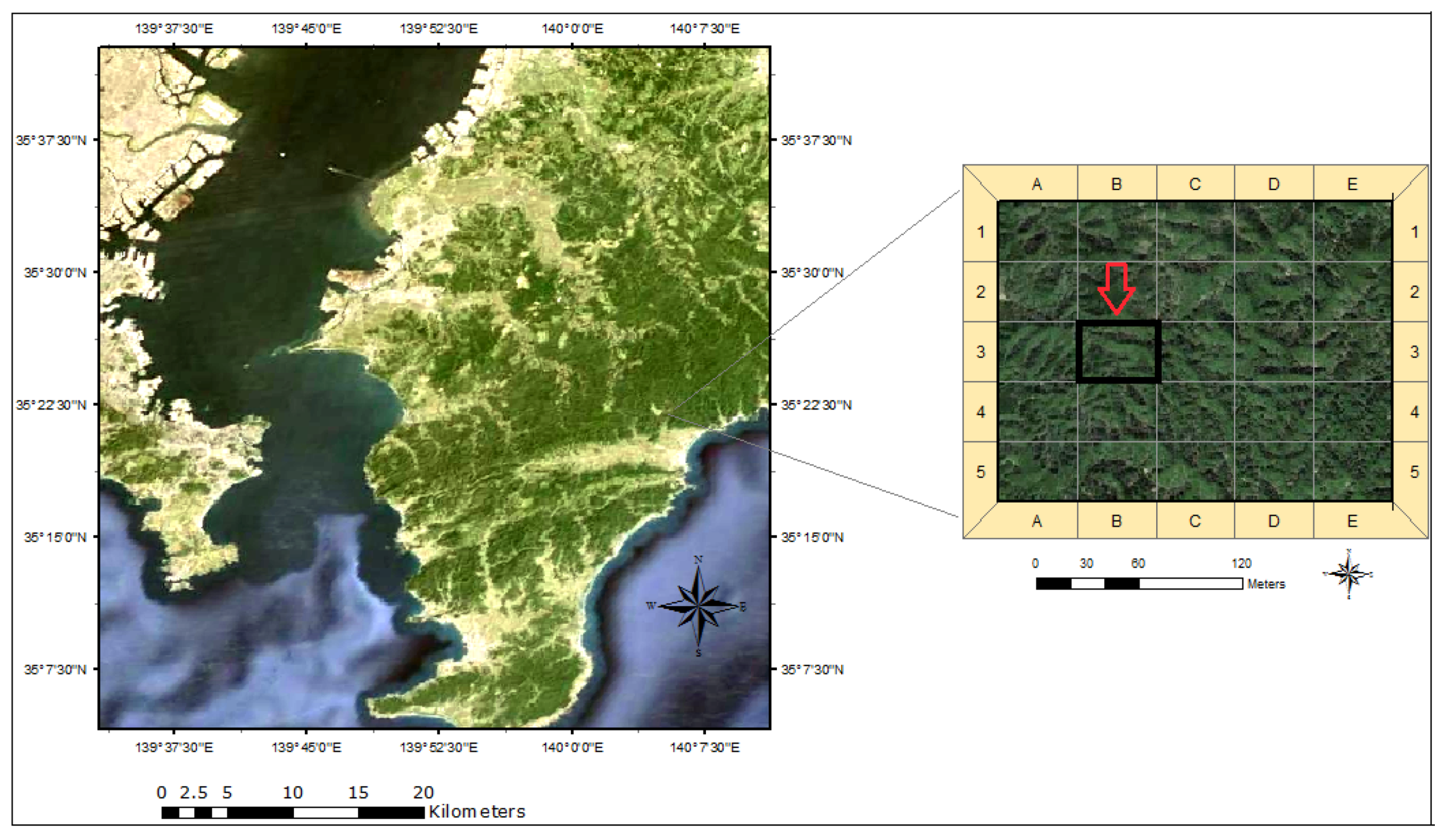
2.1. Study Area

The research area is located at the University of Tokyo Chiba Forest (UTCBF) Prefecture, Japan, located in the south-eastern part of the Boso Peninsula (Figure 1). It extends from 140° 5’33” to 10’10”E and from 35° 8’25” to 12’51”N. The forest is composed of various types of forest stands, including Cryptomeria japonica (L. f.) D. Don, Chamaecyparis obtusa (Siebold and Zucc.) Siebold and Zucc. ex Endl., Abies spp., Tsuga spp., and other evergreen broad-leaved trees. 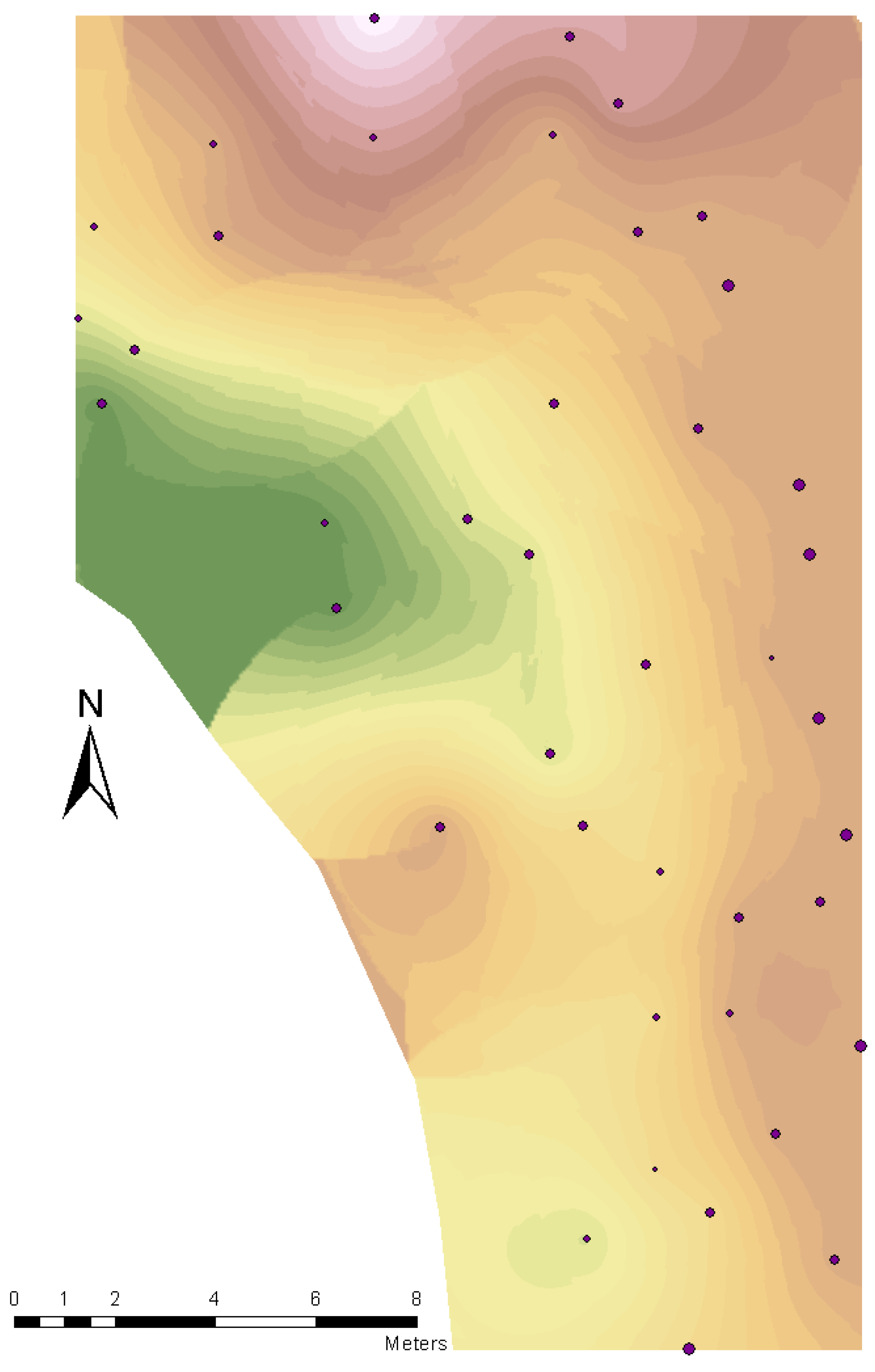The plot detail is displayed in Figure 2 with the digital terrain model based on the Z-axis measurement. We selected 20 trees for measurement within a pure stand of C. japonica with different diameters, slope, and light.

Figure 1. Location of the research area in Chiba Prefecture, Japan (source Google Earth, detail image partially modified for enhanced brightness).

Figure 1. Location of the research area in Chiba Prefecture, Japan (source Google Earth, detail image partially modified for enhanced brightness).

Figure 2. Scheme of tree positions inside plot with the digital surface model based on their Z position.

Figure 2. Scheme of tree positions inside plot with the digital surface model based on their Z position.

2.2. Photo Reconstruction

The photos were taken using a Sony NEX 7 digital camera with a fixed zoom lens of focal length 28 mm. The aperture was fixed to f/8.0, the shutter time was measured relative to the light conditions of the scene, and a flash was used because of the dense canopy and limited light penetration to the understory. However, in other (unpublished) datasets we verified that the flash is not necessary for accurate reconstruction; the potential problem that occurs in certain light environments on the stem (the illuminated and the shaded side) can be solved by using point exposure measurements with this point placed on the stem. We took approximately 20 photos regularly distributed around the stem, each of which included a view of the ground, and the distance was approximated to ensure that the stem represented approximately one-third of the photo. The distance from the camera to the tree was between 1 to 2 m, with a corresponding spatial pixel resolution of approximately 0.2–0.5 millimeters on the stem. The settings were selected in consultation with the Agisoft Photoscan © software support team. We then took an additional ring of 20 photos including the breast height (1.3 m) portion of the stem and above in order to cover a larger part of the stem. We used Agisoft PhotoScan © for image alignment, and the sparse and dense point cloud reconstruction. The mesh was reconstructed from the dense field, and the texture was mapped with density 4096 × 2 (option offered in Agisoft PhotoScan ©). The reference points were then identified on the texture model and the real world positions from measurements were attributed to them without using geometrical rectification of the model.

2.3. Field Measurement and Comparison

The trees were measured in the field including their XYZ positions (Figure 2), the circumference at breast height (1.3 m) and the height. The models produced by Agisoft Photoscan © were imported into 3D processing library for .NET environment (Devdept Eyeshot) and cross-sectional areas at 1.3 m were produced. The area of each cross-section and its perimeter (circumference) was annotated. The root mean square error (RMSE) between the circumferences measured in the field and those obtained by photo reconstruction was calculated using the following variable

$$RMSE=\sqrt{\frac{{{\displaystyle \sum }}_1^{\mathrm{n}}{\left({\text{CBH}}_{\mathrm{p}}-{\text{CBH}}_{\mathrm{f}}\right)}^2}{\mathrm{n}}}$$

(1)

where the $CB{H}_p$ is the circumference at breast height from the photo model and $CB{H}_f$ is the circumference at breast height from the field measurements. The n is the total amount of samples.

2.4. Magnetic Digitization

Next we analyzed the error using the digitized points and their distances from the photo reconstructed model. The digitization of these control points was implemented using a newly developed method similar to [32]. We collected surface data with a magnetic motion tracker, POLHEMUS FASTRAK^®. We used FastrakDigitizer^® software, as described in [25], with a TX4 source mounted on a wooden tripod avoiding the points to be measured at the edge of the magnetic field, where the accuracy according to [33] might be lower The manufacturer reports accuracy to be submillimeter (more precisely 0.03 inches (0.7 mm) Root Mean Square Error (RMSE) for the X, Y, or Z positions [33]). The system has an operational range of approximately five feet with the standard source, seven feet with the TX4 source, with the option to extend the field of range up to 10 feet (using Long Ranger extension). FASTRAK^® provides both position and orientation data measuring requirements of applications and environments with no need for additional calculations.

For each stem, we recorded the horizontal contours around the stem at each change in curvature or more significant changes in the stem’s thickness to a height of approximately 3 m (the lower part of the stem) We marked the north and the vertical (horizontal) direction for post-processing orientation of the model. Six reference points regularly distributed along the stem were also assigned for later alignment with the photo model. The coordinates of these points were used as reference points in Agisoft Photoscan © for georeferencing the point cloud and 3D mesh. The magnetic digitizer uses a source with [000] so the points are referenced in this local coordinate system. During the photo reconstruction, we attempted to recover the texture precisely, e.g., with high detail. The model referenced in local coordinate system was exported and further processed in FastrakDigitizer in order to calculate the displacement of each point and average displacement compared to the digitized points.

2.5. Error Term—Minimum Distance and Morphology

The error was defined as the shortest distance of the digitized point to the photo reconstructed model. The algorithm for finding the smallest distance begins by searching for the closest vertex of the model. Once that vertex is found, it tests whether any of the triangles of the mesh, where this vertex is one of the vertices of the triangle, has a perpendicular distance to the testing point shorter than the distance to the vertex; if any exist, that shortest distance then becomes the distance error.

The morphological error was defined as the difference between the perimeter and cross-sectional area of the stem reconstructed from the magnetic measurement and from the photo-reconstruction. Each of the models is sectioned horizontally in a vertical direction, and then the values of the perimeter and area are compared for each cross-section. The distance error described above is a non-negative value, i.e., the distance is directed to either the outside or inside of the mesh surface (it may be also understood as absolute magnitude of the error). The reason we tested for the morphological error is that the displacement error may result from either of two different situations which can be also referred to as systematic and random errors: the random in which all points are alternatively found outside and inside of the true stem (no morphology error), and the systematic in which all points are found either outside or inside the stem (resulting in clear morphology error).

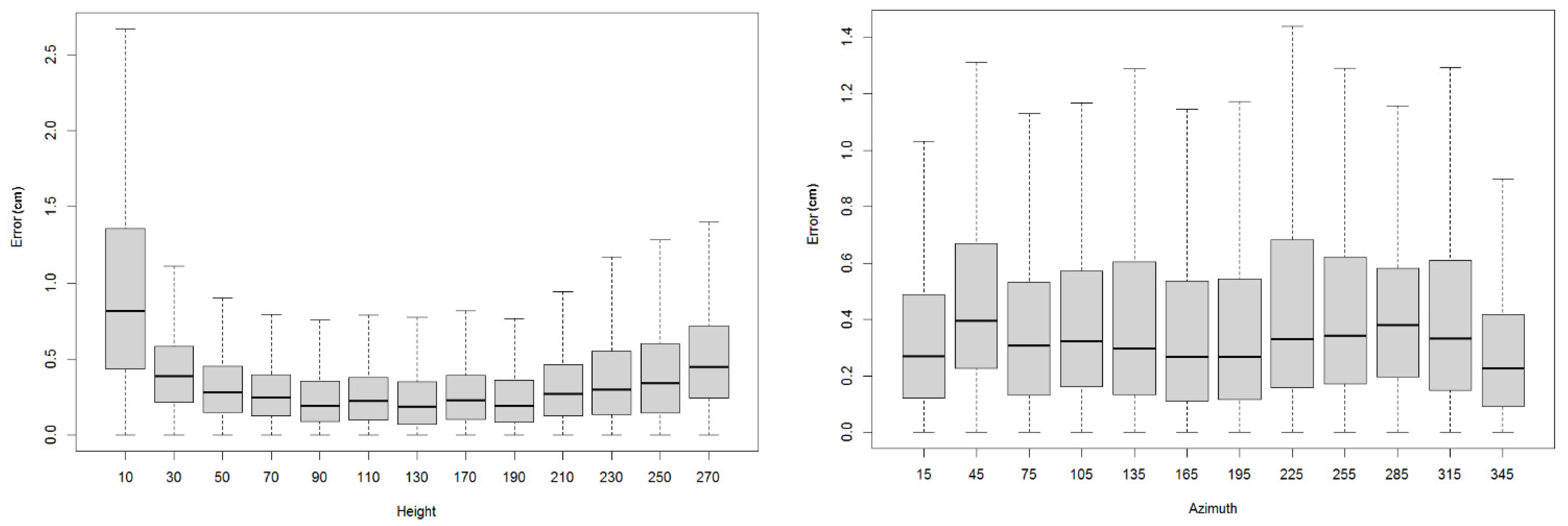
The results were analyzed in three steps. In step 1 we conducted the point-based analysis and compared the distance between the individual control points and the photo model. We investigated how the minimal distance correlated with the height of the control point on a stem and how it correlated with the azimuthal angle relative to the north position.

We hypothesized that the texture, particularly the presence or lack of lichens on northern and southern sites, respectively, may potentially influence the error on some sites. We used the circular statistic in the R statistical software for this analysis [34]. However, the behavior of the linear variable over the azimuth (circular) variable is better described by cylindrical statistics as a sub-area of circular statistics [34]. The cylinder shape was best approximated the texture data, and therefore we used cylindrical statistics to model stem texture. We used the Johnson-Wehrly-Mardia correlation coefficient to test the correlation between the azimuth and the angle [34].

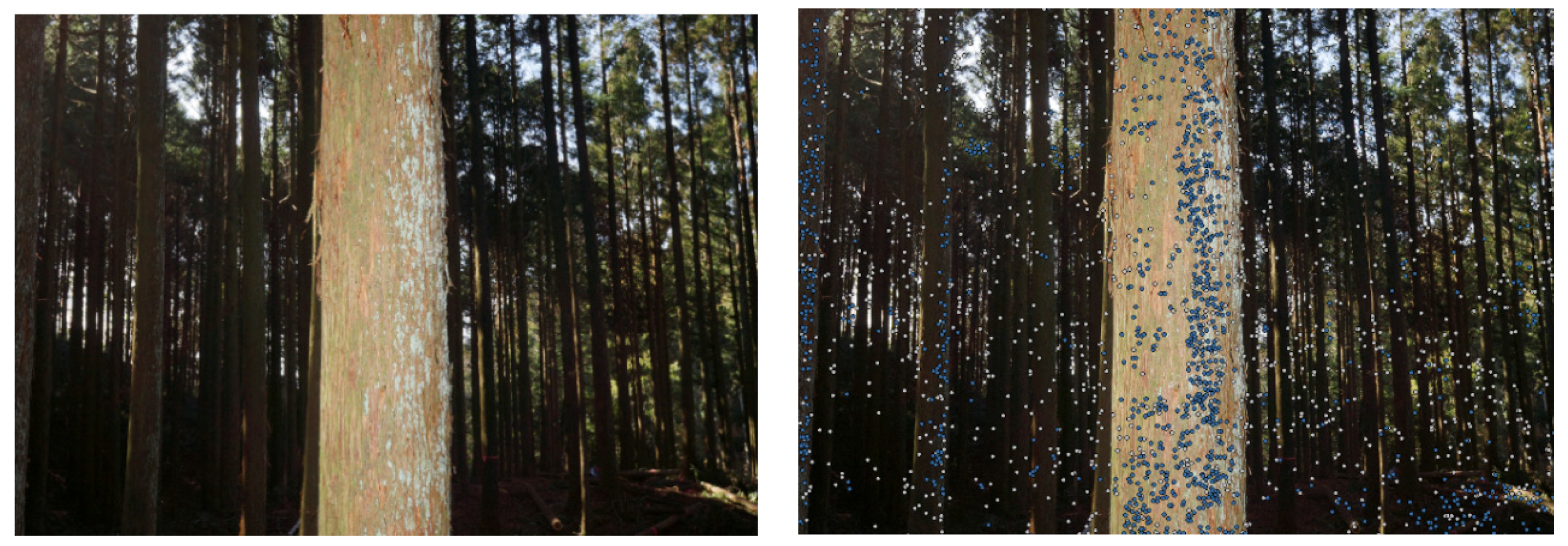
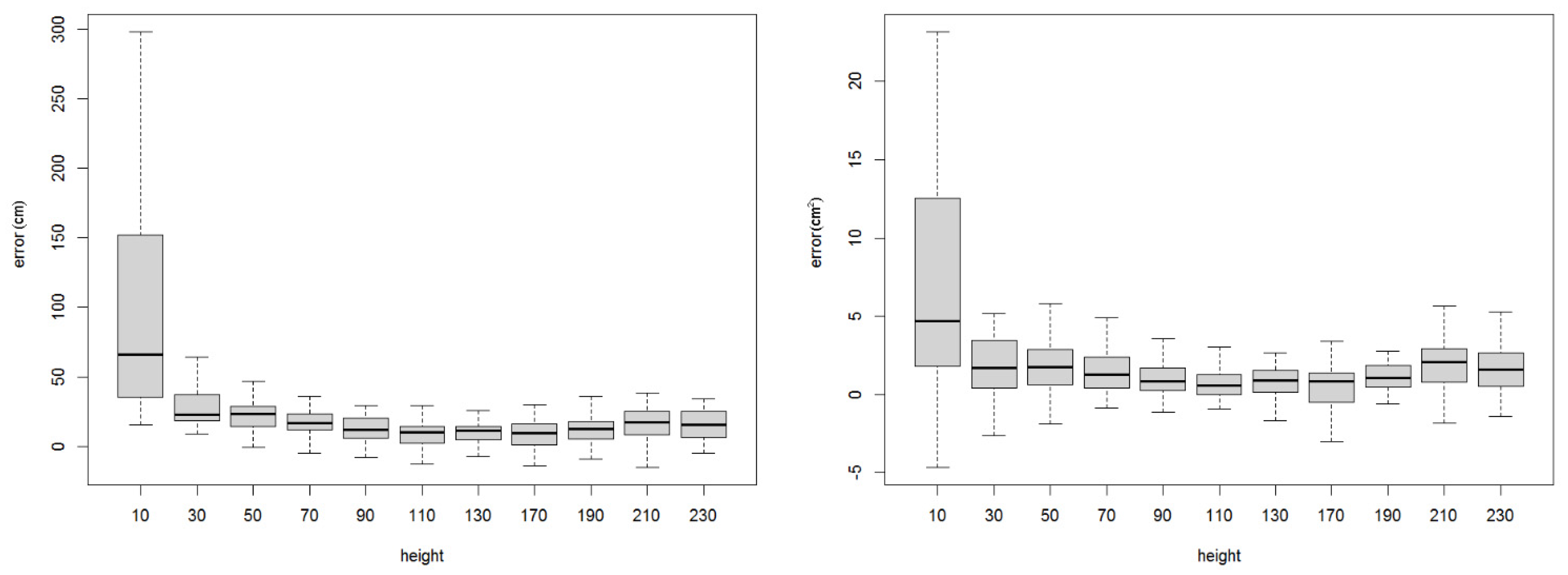
The left panel of Figure 3 shows an example of the typical surface texture of a C. japonica stem. The presence of the lichens on the northern portion of the stem supported a hypothesis for better performance of the algorithm on the northern site. However, the right panel of Figure 3 shows that in the lower part of the stem, the detected points are also present in non-northern portions of the stem. Other possible features that may hypothetically influence accuracy might include tree age, season, or stem conditions, all of which may be examined in a future study. Step 2 was the analysis of morphological characteristic based on the stem perimeter and horizontal cross-section. Because the error distance is always positive, it is difficult to distinguish the direction of the error, either outside or inside the stem. The analysis of cross-sectional differences reveals the direction of the distance error; in this case we used the squared value of the difference.

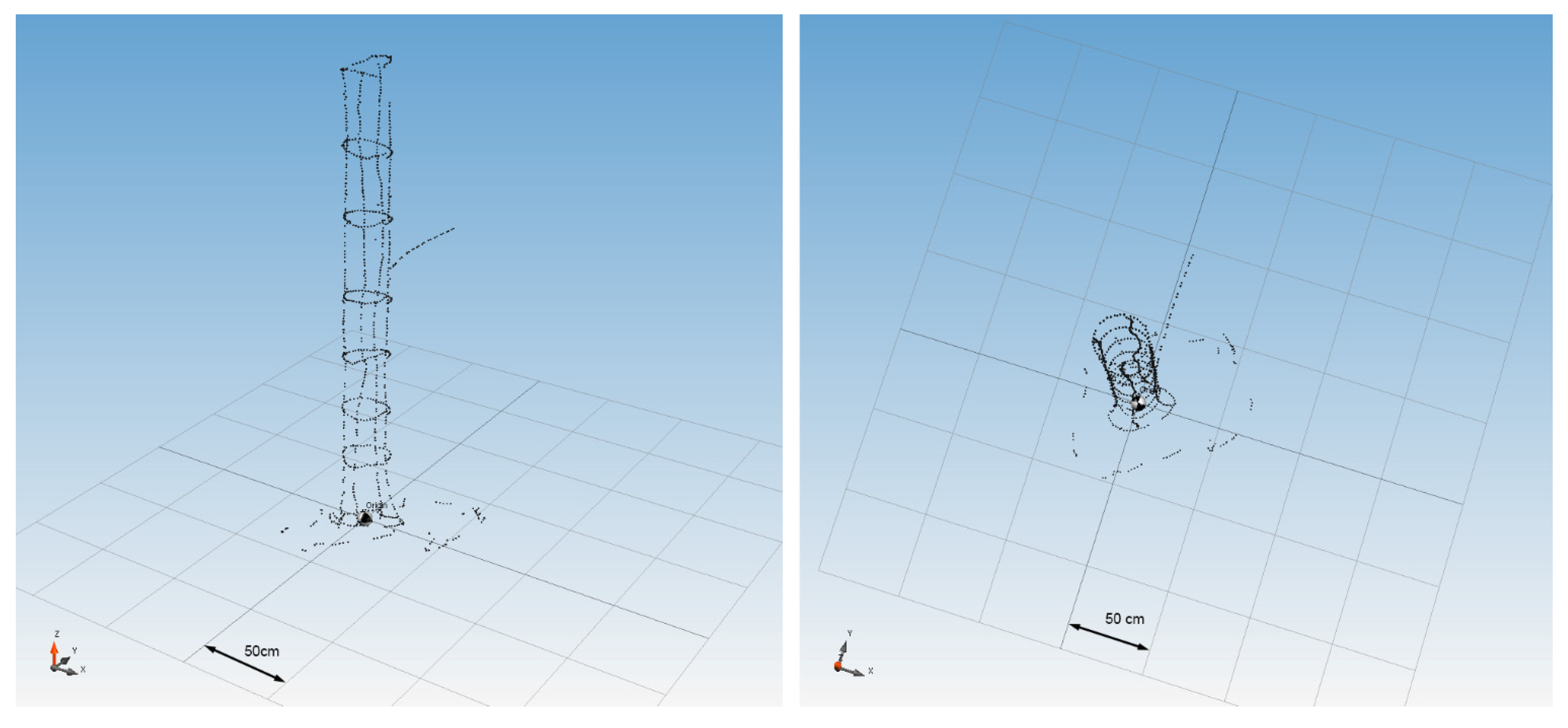
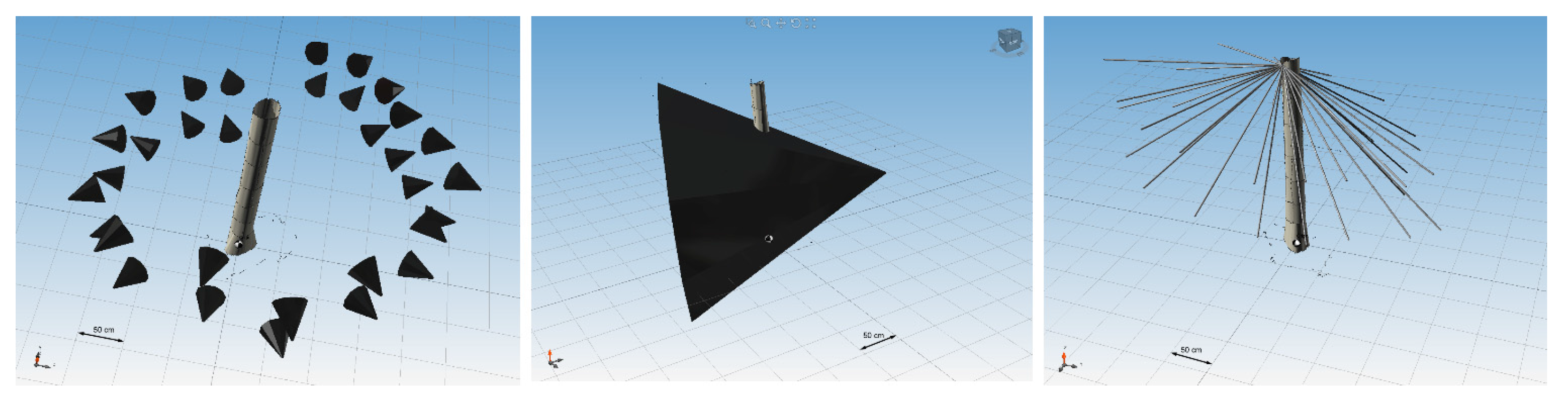
Step 3 was to analyze the mean error from individual points with relation to the number of cameras able to capture a designated focal point. The number of cameras was determined by two factors: whether the point was inside the camera’s field of view, and if the point could be seen by the camera. To determine if a point was in the camera’s field of view, we specified each camera position based on its xyz coordinates and the rotation of a cone whose peak is situated in the camera position; the rotation was defined by the camera rotation (Figure 4, left). The height (length) of the peak was defined as any large number exceeding any possible position of the control points. We then calculated whether the camera could view the points through overlapping stems. The contour points were collected all over the surface, but they were partially hidden for each camera. This can be easily verified as shown in Figure 4 (right).

Figure 3. Surface data collected from a tree stem surface by a magnetic motion tracker.

Figure 3. Surface data collected from a tree stem surface by a magnetic motion tracker.

On the left-hand side of Figure 4 are the positions, rotations, and angle of view for every position of a camera around the stem. The middle figure of Figure 4 shows the area of the stem covered by a camera from one position, which was used to calculate the amount of cameras theoretically seeing the point. The right-most figure of Figure 4 shows the connection of a camera with individual points and the reconstructed surface of the stem. Those cameras, from which the connecting line crosses the stem’s surface, are eliminated from the total amount of cameras seeing points.

Figure 4. Example of typical surface texture of Cryptomeria japonica and the points automatically detected by Agisoft Photoscan © software.

Figure 4. Example of typical surface texture of Cryptomeria japonica and the points automatically detected by Agisoft Photoscan © software.

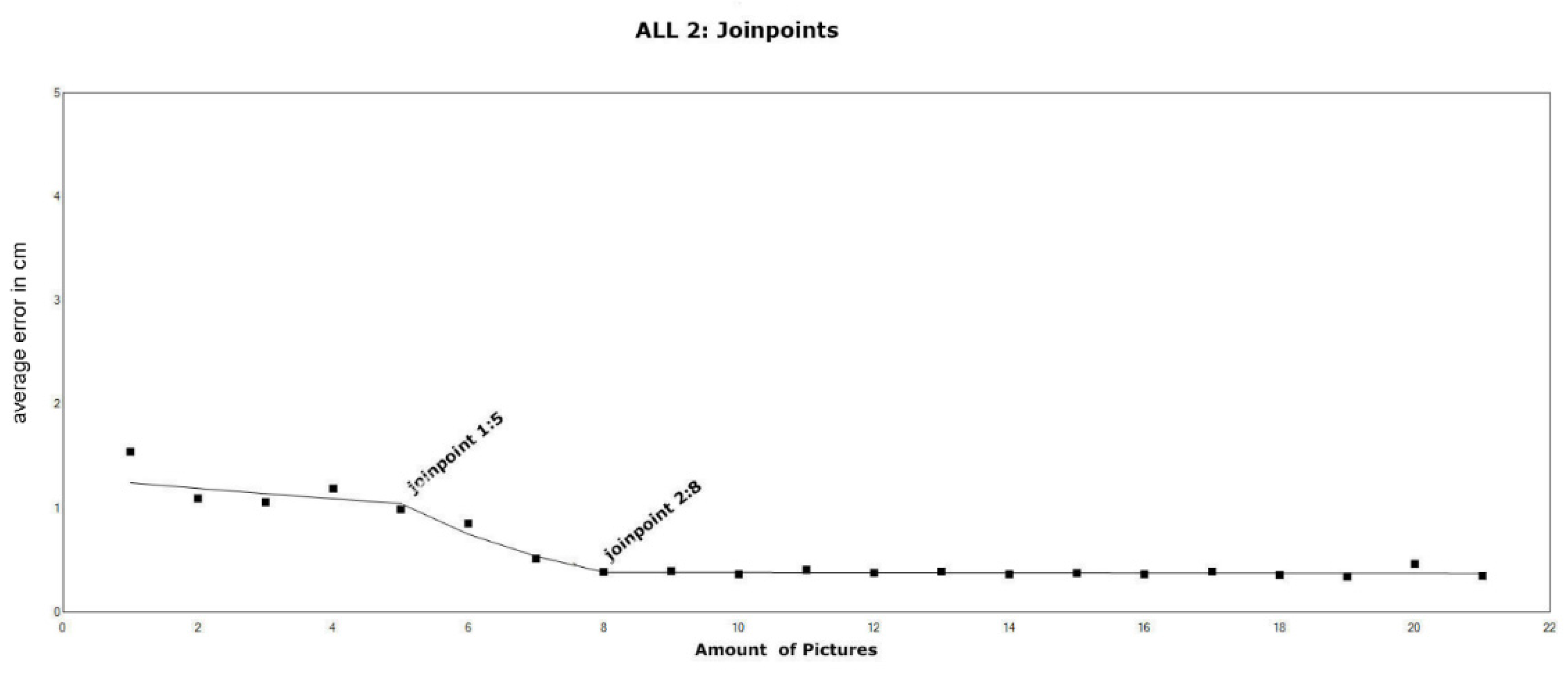
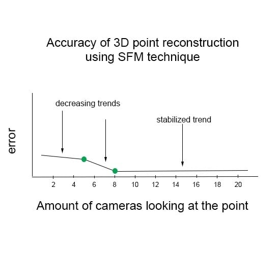
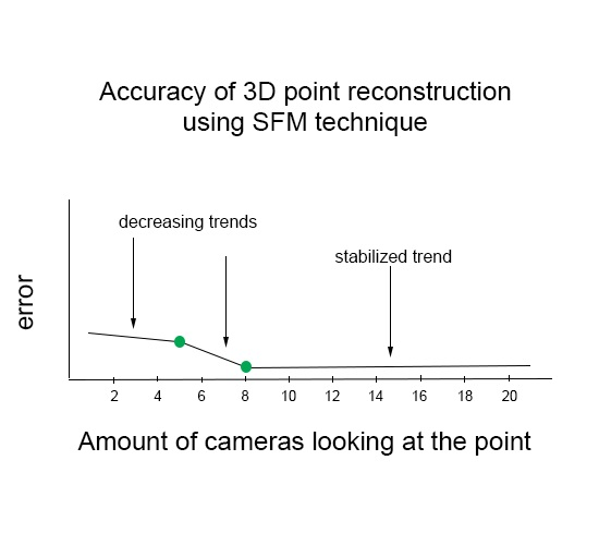
2.6. Trend Detection

To evaluate the trend of errors associated with the number of cameras, it was expected that the error value would decrease with the increasing number of cameras pointing at the point on the stem, and beyond a certain number of cameras the error would be stabilized. We attempted to identify the ideal number of cameras that would stabilize the associated error of point location accuracy. We used the method by [35] to analyze the trend in our data using joinpoint models, which utilizes different linear trends connected at certain points; these are termed as “joinpoints” by the authors. The “Joinpoint Trend Analysis Software” evaluates the trend data and fits the joinpoint model, starting from the minimum number of joinpoints to the user-defined maximum; we used a value of 0 as a minimum and a maximum value of 10. Significance is tested using the Monte Carlo permutations method, and for each number of joinpoints, the software estimated significance values for the amount of joinpoints and for each of the partial linear trends.

3. Results

3.1. Accuracy of Diameter Estimation from Photo Reconstructed Shapes

We evaluated the accuracy of photo reconstructed stems and compared them to the common field measurement of stem circumference using measuring tape at breast height (1.3 m). The root mean square error (RMSE) and its deviation is displayed in Table 1. The error of circumference measured by tape was 1.87 cm different from the one measured on the photo models; however, its variability was rather high (2.23). The difference in circumference represents a corresponding error of 0.59 cm in diameter.

Table 1. The root mean square error (RMSE) of circumference in breast height (CBH) calculated from photo reconstructed models and the terrain measurement using common dendrometric tape, and RMSE of diameter in breast height (DBH). Both values include standard deviation (SD).

RMSE CBH (cm)	SD (cm)	RMSE DBH (cm)	SD (cm)
1.87	2.23	0.59	0.72

Table 1. The root mean square error (RMSE) of circumference in breast height (CBH) calculated from photo reconstructed models and the terrain measurement using common dendrometric tape, and RMSE of diameter in breast height (DBH). Both values include standard deviation (SD).

RMSE CBH (cm)	SD (cm)	RMSE DBH (cm)	SD (cm)
1.87	2.23	0.59	0.72

3.2. Accuracy of Point Reconstruction

The analysis of the accuracy of the individual point reconstruction is divided into the following parts: analysis of point error in vertical and horizontal directions, morphological analysis of error, e.g., the systematic error, and analysis of image overlapping here described as the number of cameras seeing a point.

3.2.1. Displacement Error and Its Distribution in Vertical and Horizontal Directions

As evident on the left side of Figure 5, when comparing the error by height, the error in the middle portion of the stem was lowest, and it was higher at the base and crown of trees where the degree of visibility and the ability of the optical sensor for capturing an image were low. Based on the azimuth (right figure of Figure 5), it appeared that the error was lower on the northern face of the stems, although differences were not statistically significant. The Johnson-Wehrly-Mardia correlation coefficient [34] resulted in a $R_{x\theta }^2$ coefficient of 0.0094 with a p-value for the test of independence equal to 0.0680; the low value of $R_{x\theta }^2$ suggests that the correlation of error size and azimuth was very low.

Figure 5. Left: the positions of individual cameras with their rotations and field of view, middle: the angle of view of one camera, right: the connections of point to all cameras for determination of visibility.

Figure 5. Left: the positions of individual cameras with their rotations and field of view, middle: the angle of view of one camera, right: the connections of point to all cameras for determination of visibility.

3.2.2. Morphological Error and Accuracy of Stem Morphology

Figure 6 shows the morphological error, defined by stem circumference (left panel) and cross-sectional area (right panel), in relation to the height at 20 cm increments. Similar to the point error analysis, the error was highest at the bottom and upper portions of the stem model and lowest at the breast height portion of the stem where the area of overlap of the individual images was highest.

Figure 6. Error (cm) and its distribution with height (left) and azimuth (right).

Figure 6. Error (cm) and its distribution with height (left) and azimuth (right).

3.2.3. Influence of the Number of Cameras and Related Precision

The model with two joinpoints was found to be the best (Table 2); other models (with joinpoints of zero and three) were considered not significant or less significant than this one. Figure 7 shows the results of the analysis on trend tendency and determination of joinpoints. The two joinpoints considered significant occurred at five cameras and eight cameras (Table 3). All three segment slope estimates were significantly negative, and the most significant decrease was observed in the second segment (Table 4), between five and eight cameras, thus implying that shape reconstruction error significantly decreased for every camera added beyond five cameras only up to eight cameras, where the slope essentially become zero. Beyond a total of eight cameras, the error stabilized, meaning that adding more cameras (views) would not improve the performance (Figure 8).

Table 2. Model statistics.

Cohort	Number of Joinpoints	Number of Observations	Number of Parameters	Degrees of Freedom	Sum of Squared Errors	Mean Squared Error	Autocorrelation Parameter
All	2	21	6	15	0.182	0.012	Uncorrelated

Table 2. Model statistics.

Cohort	Number of Joinpoints	Number of Observations	Number of Parameters	Degrees of Freedom	Sum of Squared Errors	Mean Squared Error	Autocorrelation Parameter
All	2	21	6	15	0.182	0.012	Uncorrelated

Figure 7. The error in circumference (cm) by height (left) and stem sectional area (cm²) by height (right).

Figure 7. The error in circumference (cm) by height (left) and stem sectional area (cm²) by height (right).

Table 3. Estimated joinpoints with corresponding confidence limits (CL).

	Joinpoint	Estimate	Lower CL	Upper CL
All	1	5	3	7
All	2	8	7	10

Table 3. Estimated joinpoints with corresponding confidence limits (CL).

	Joinpoint	Estimate	Lower CL	Upper CL
All	1	5	3	7
All	2	8	7	10

Table 4. Estimated regression coefficient (general parameterization).

	Parameter	Parameter Estimate	Standard Error	Test Statistic	p-Value
All	Intercept 1	0.2632	0.1408	1.869	0.084
All	Intercept 2	1.7074	1.1136	1.533	0.149
All	Intercept 3	−0.9348	0.1322	−7.067	0.000
All	Slope 1	−0.0437	0.0497	−0.878	0.395
All	Slope 2	−0.3325	0.1745	−1.905	0.079
All	Slope 3	−0.0022	0.0082	−0.275	0.787

Table 4. Estimated regression coefficient (general parameterization).

	Parameter	Parameter Estimate	Standard Error	Test Statistic	p-Value
All	Intercept 1	0.2632	0.1408	1.869	0.084
All	Intercept 2	1.7074	1.1136	1.533	0.149
All	Intercept 3	−0.9348	0.1322	−7.067	0.000
All	Slope 1	−0.0437	0.0497	−0.878	0.395
All	Slope 2	−0.3325	0.1745	−1.905	0.079
All	Slope 3	−0.0022	0.0082	−0.275	0.787

Figure 8. The trend analysis of the data. The error on y-axis, the amount of cameras that see the focal point on x-axis.

Figure 8. The trend analysis of the data. The error on y-axis, the amount of cameras that see the focal point on x-axis.

4. Discussion

The recent advances in computer vision allow accurate reconstruction of the terrain surface from remotely sensed images (e.g., [29]) and they can also be used for reconstruction of individual 3D objects (as demonstrated in this study). This reconstruction method has great potential, especially when compared to the commonly used laser scanning methods. Although laser scanning methods are most likely more precise and create more points from fewer positions, the high cost of equipment is currently restrictive. Using the uncalibrated cameras, the photo reconstruction is possible with any mid-level commercial camera, and the processing is possible using several different software types, some of which are even freeware. However, the usage of calibrated cameras (even calibrated with freeware software) can only enhance the model as demonstrated, for example, in [36]. Recently, optical cameras are mostly being deployed on Unmanned Aerial Vehicles for extraction of inventory parameters, e.g., [37,38]. An overview of possible usages is demonstrated, for example, in [39].

In this study we used the handheld camera to create the three-dimensional models of stems using the recommended settings from the software manufacturer. The resulting stem objects are visually realistic, and comparing them to the field measurement we obtain the RMSE of 1.87 cm in circumference at breast height. However, this value has large variability and when viewing the object as a remote-sensed surface model we designed a method for evaluation of the accuracy at individual points spread on the stem.

The study in [31] used differential GPS (DGPS) technology as the ground truth data to verify the accuracy of point clouds from photos, and they concluded that terrain reconstruction accuracy was around 2.5 to 4 cm provided that the ground control points were clearly visible, well contrasted with the surrounding landscape, and sufficiently spread around the investigated scene. They also concluded that the flight planning must ensure a high degree of overlapping (at least 70% of the images); however, the flight altitude is generally considered to be the most critical factor for the recognition of individual features. The use of DGPS is limited inside a forest canopy, though, mostly because the GPS signal is weak under a dense canopy. Other authors have used data from the total station as the ground reference data. For instance, [39] stated that the use of total station provided accuracy with an error of approximately 1 cm in horizontal position and about 2 cm in vertical position (elevation). The studies [40,41] used total station ground-truthed data to assess the accuracy of LiDAR, and [42] used it to assess the accuracy of GPS.

A magnetic motion tracker provided the reference data in this study. A series of overlapped images were photographed around the individual trees in the sample plot using a hand-held camera. A point cloud was generated from these images for each stem, and they were used to construct the mesh object with high-resolution texture in Agisoft Photoscan © software. This model allowed the usage of reference points measured by the digitizer to be referenced in the local coordinate system.

We used the other points to evaluate the accuracy of the model and found that the accuracy is not significantly dependent on the presence or lack of lichens (typically present on the north part of the stem), but we found that the accuracy is decreasing and again increasing in height. We evaluated the newly introduced term “amount of cameras which see the point” which refers to the degree of overlapping for such a point and we found that the higher this degree of overlapping, the better the precision will be. In general we found in our data that when the amount of cameras goes beyond eight there is no further increase in accuracy.

5. Conclusions

We evaluated the suitability of a handheld camera for the reconstruction of the tree stem surface using the recommended settings from the manufacturer of the software Agisoft PhotoScan © which are based on the algorithms deployed in it. We found the RMSE error of circumference of the stem to be 1.87 cm to the field measurement with a measurement tape. Such an error represents the diameter estimation error of approximately 0.59 cm which can be considered rather good for inventory purposes; however, the large variability (standard deviation) of this error led to a more detailed error study based on control points from the magnetic motion tracker. The magnetic motion tracker allows the measurement of points which are hidden from the source of the magnetic field (e.g., those behind the stem).

When compared with control points, we determined that if five or more cameras could see the points, the error decreased significantly; however, eight or more cameras did not appreciably lower the error. Based on these observations we can conclude that terrestrial multi-view photography may be a promising method for forest inventory as it can provide reliable estimates for the diameters at breast height but also the additional diameters at different heights.