1. Introduction
The prevailing analysis and synthesis of climate models [
1,
2] project that a persistently increasing trend of aridity dominates the global climate change in the 21st century despite a short period of cooling over the past 17 years. Frequent and severe droughts would put many forest ecosystems under significant moisture stress, with severe consequences for the ecosystem structure and function [
3,
4,
5]. Because of the increased droughts and heat waves, the global net primary productivity (NPP) has been found to decrease in the new century [
6], and tree mortality has been found to increase [
7] in many places around the world. Ecosystems with drought resistance and tolerance, such as shrubs [
8], may become increasingly prominent in the future.
Shrubs have been reported to expand to arid, semiarid, and sub-humid regions [
9,
10,
11,
12] and to invade arid and semiarid grassland [
8,
13]. The expansion of shrubs in grassland has complicated the consequences of ecosystem structure and function. For instance, the invasion of shrubs in arid grassland reduced ecosystem production and carbon sequestration [
14]. However, recent studies have indicated that shrub encroachment has positive effects on the ecosystem functions of herbaceous biomass [
15], microbe diversity, and nitrogen mineralization [
16]. Based on the experiment in southeast Spain [
17], shrub encroachment has been found to increase soil organic carbon, total nitrogen, and biological soil crusts. Instead of leading to desertification in previous studies, shrub encroachment is considered to reverse desertification in the Mediterranean grasslands [
17].
The superior tolerance of shrubs to moisture stress can be attributed to their small leaf-to-sapwood-area ratio [
18,
19] and their deep rooting profile [
20,
21]. Because of the lack of a main trunk and their multiple branches, the leaf-to-sapwood-area ratio of shrubs is on the order of 10
3, whereas the ratio for arbores is within the order of 10
5 to 10
6 [
22,
23]. The stomata of shrubs is more resistant to moisture stresses in both soil and air compared to that of other functional types [
24,
25,
26,
27]. Therefore, shrubs should perform better than other functional types in the global drying trend.
Spatiotemporal patterns of vegetation performance have been measured by various satellite remotely sensed vegetation indices, among which the enhanced vegetation index (EVI) from the MODIS sensor (Moderate-Resolution Imaging Spectroradiometer) has the best linearity with the green biomass (mostly leaf) of the Earth [
28]. EVI has been widely used to monitor and measure vegetation growth status [
29,
30], primary productivity [
31,
32,
33,
34,
35,
36,
37], evapotranspiration [
38], and plant phenology changes [
39].
The seasonality of the climate has been considered to be an important modifier of grass-shrub competition. Shrubs sensed warming in the spring earlier than grasses due to the shrubs higher buds in the air, and warm spring favored shrubs during leaf out [
8]. Warming tends to shorten the growing season of mono-cultivated crops; however, it has been found to prolong the growing season of multispecies ecosystems [
40]. The rainfall seasonality might be the most important driver, and shifting rainfall from summer to other seasons favors shrubs rather than grasses [
41].
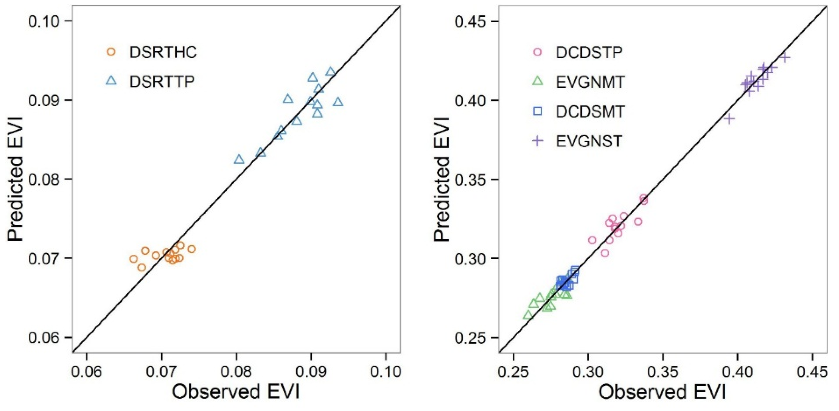
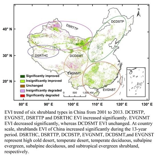
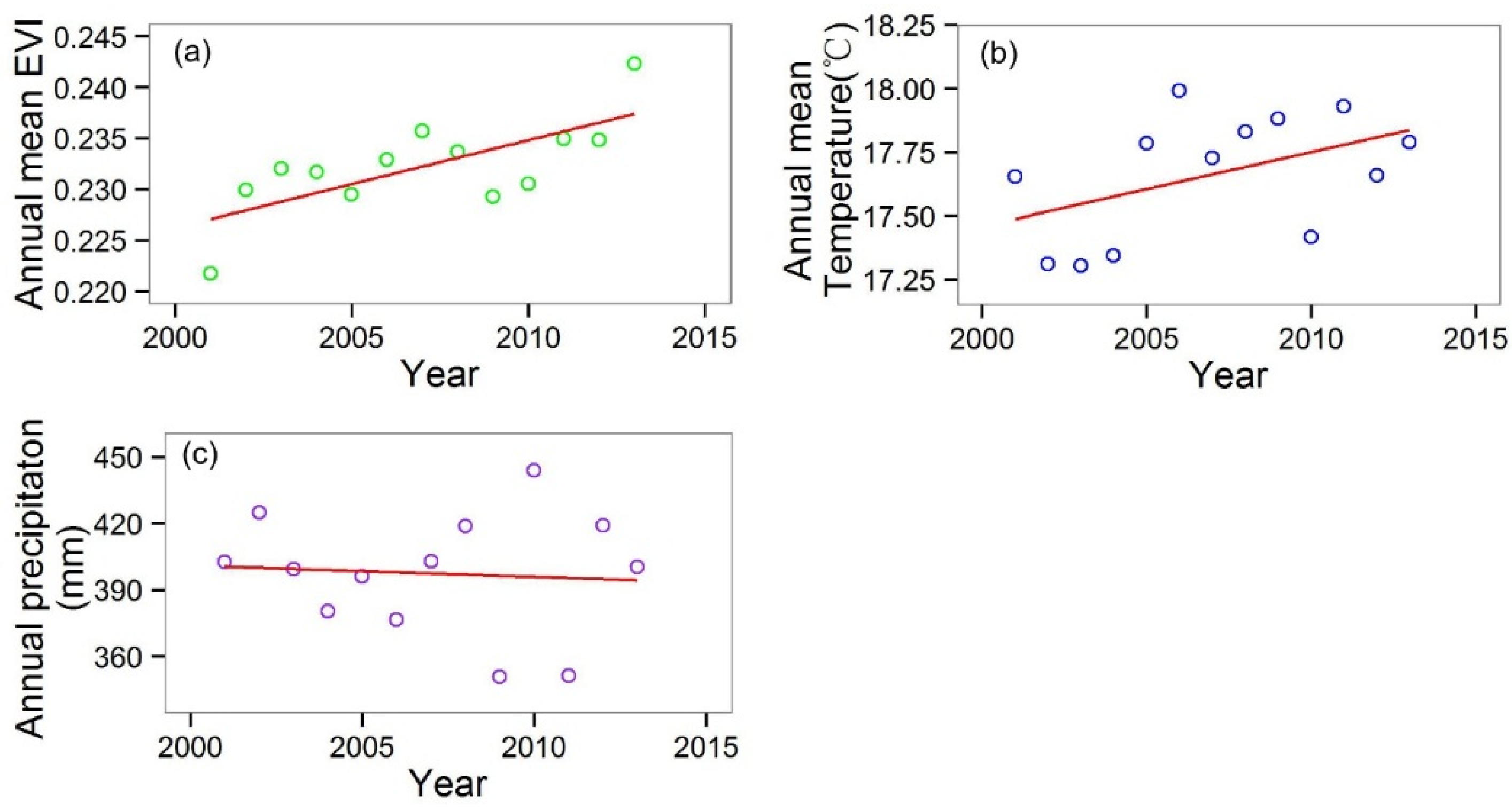
Shrublands occupy more than 20% of the land in China [
42] and can be classified into six functional types: subtropical evergreen (EVGNST) in the south; temperate deciduous (DCDSTP) in the north and northeast; subalpine evergreen (EVGNMT) and subalpine deciduous (DCDSMT) in the east slopes of the Tibet; temperate desert (DSRTTP) in the north and northwest; and high-cold desert (DSRTHC) shrublands in the west of Tibet. EVGNST is dominated by subtropical/tropical evergreen broad-leaved shrubs mixed with a small deciduous component. DCDSTP and DCDSMT are dominated by deciduous broad-leaved shrubs. EVGNMT is composed of a majority of sclerophyllous evergreen broad-leaved shrubs and a small part of evergreen needle shrubs. DSRTTP is dominated by temperate subshrubs and temperate desert shrubs, while DSRTHC is dominated by high-cold cushion subshrubs. EVGNST (the second largest in area) and DCDSTP have the best climate conditions and thus the largest average EVI of 0.429 and 0.321, respectively. On the other hand, the two desert shrublands (DSRTTP and DSRTHC) have the smallest average EVI of 0.088 and 0.071, respectively, despite the greatest distribution area of 1,068,218 km
2 of the former. The two sub-alpine shrublands have relatively small distribution areas and moderate average EVI values. Thus, the countrywide average EVI and its temporal patterns are mostly contributed by EVGNST and DCDSTP. The contribution of shrublands to the NPP in China has been found to be comparable to the arbores forest [
43]. Shrublands in China expanded in this century because of the policy-guided shrub planting after abandonment of crops in northern China [
44,
45]. While EVI in China has been found to increase in a non-significant manner [
46], we expected that the shrubland EVI should have a stronger increasing trend than the overall EVI in China.
The objective of this study is to test three hypotheses: (1) the annual average EVI in China Shrublands significantly increased from 2001 to 2013; (2) intra- and inter-annual changes in temperature and precipitation greatly altered the growing season of shrublands; and (3) the significant increase in shrub EVI can be explained by the extension of the growing season and the favorable climate. We analyzed the annual and seasonal EVI at both pixel-based and shrubland type scales to derive the trends in annual/seasonal EVI and climate variables, as well as the trends of the growing season length, and quantified the relationship between the trend in EVI and the climate variations and the growing season length.
2. Materials and Methods
2.1. Data Acquisition and Preprocessing
We obtained the MODIS EVI that covers continental China over the period from 2001 to 2013, with a spatial resolution of 1 km and temporal resolution of 16 days, from the NASA Data Center [
47]. Firstly, we applied the approach suggested by Samanta
et al. [
48] to screen for good data. Secondly, we temporally filled the missing or unreliable EVI based on the quality assurance flags using a simple linear interpolation [
49]. Then, we aggregated the monthly EVI by applying the maximum value composite (MVC) method to the two images from each month. Finally, based on the 1:1 million vegetation map [
42], we extracted the EVI for the subtropical evergreen mixed with a small part of deciduous (EVGNST), temperate deciduous (DCDSTP), subalpine evergreen (EVGNMT), subalpine deciduous (DCDSMT), temperate desert (DSRTTP), and high cold desert shrublands (DSRTHC). Furthermore, pixels with an annual mean value less than 0.05 were excluded to reduce the impact of bare soil and too sparsely vegetated pixels [
50].
To explain the changes in EVI, we obtained the monthly temperature and precipitation records of 659 meteorological stations across China from the Meteorological Data Center for the same period of time [
51]. The monthly temperature and precipitation were then interpolated to all of the shrublands using Kriging. The monthly EVI, temperature, and precipitation maps were spatially averaged over the six shrubland types and then averaged seasonally and growing seasonally to obtain the times series of the EVI and the climate variables. Our study focused on the growing season (from April to October), which can be divided into three seasons: spring (April and May), summer (June, July and August) and fall (September and October) [
50,
52]. To explore the effects of winter climate change on the starting days of the growing season, we defined winter as November of the prior year to March of the following year [
53].
2.2. Growing Season Length Detection
To explore the temporal trend of the growing season for each shrubland type, the TIMESAT program was used to obtain the profile of the 16-day EVI time series using asymmetric Gaussian functions [
54]. TIMESAT program is a common tool for phenology detection by setting a threshold value to determine the start of the season and end of the season [
30,
55,
56]. The start of the season was defined as the point at which the EVI increased to a value that was set to 30% of the distance between the minimum and maximum of the left edge. Similarly, the end of the season was defined as the point at which the EVI decreased to 30% of the distance between the minimum and maximum of the right edge. The growing season length was extracted by calculating the days between the starting day and the ending day.
2.3. Pixel-Based Non-Parametric Trend Analyses of EVI
Mann-Kendall’s test and Theil-Sen median slope were used to obtain the possible monotonic trend in the time series of the annual average EVI at the pixel level, which were widely used to determine vegetation variation [
57,
58,
59]. The Mann-Kendall’s test [
60] is a robust nonparametric significance test that calculates Z values based on the signs of changes in the time series. Z values greater than 1.96 indicates a significantly increasing trend, and a Z value smaller than −1.96 is regarded as a significantly decreasing trend.
Mann-Kendall’s test does not count the magnitude of changes between any two consecutive pairs of numbers in the time series. The Theil-Sen median estimator, βTS, is a robust simple linear regression that chooses the median of slopes calculated between any pair of data points in the time series, and hence compensates for the Mann-Kendall’s test in the quantitative aspect. This method is appropriate for assessing the rate of change in short or noisy time series because it is robust to outliers. βTS is divided into three ranges of βTS < 0, βTS = 0, and βTS ≥ 0, for “degraded”, “unchanged”, and “improved”, respectively. In combination with the three ranges of Mann-Kendall’s test, we can define two additional classes, i.e., βTS < 0 with Z < −1.96 for “significantly degraded” and βTS ≥ 0 with Z > 1.96 for “significantly improved”.
2.4. Regression with Serial-Correlation for Trends in EVI, Climate Variables and Growing Season
A more quantitative approach to time series analysis is the generalized least squares regression, which is capable of deriving the quantitative trend together with the serial correlation in the time series. Generalized least squares regression is applied to annual/seasonal EVI, temperature and precipitation, and EVI-derived growing season length in this study. To avoid spatial autocorrelation, we averaged these variables over the six shrubland types and applied the generalized least squares regression to the lumped data. We tested whether there was a significant temporal trend and quantified the strength of the trends in EVI, temperature and precipitation, as well as the growing season length of the growing seasons.
The seasonally and annually averaged EVI, climate, and growing season length variables were regressed on time using the following equation:
where y is any of the above variables, x stands for year, and a is an intercept. Slope k stands for the trend. The analysis of EVI, seasonal climate variables and growing season length will allow us to quantify the changes in seasonal profiles of these variables.
2.5. Regression of Annual Average EVI on Growing Season Length and Climate Variables
The Kriging interpolated precipitation and temperature may not reflect the true water supply and temperature of the scattered shrublands. However, the temporal trends of the interpolated climate variables should be close to those of the shrublands.
To quantify the effects of climate variations on the growing season, we regressed the growing season length on the seasonal precipitation and temperature. The annual averaged EVI (April to October) were regressed on the growing season length and selected seasonal climate variables to establish dependence of EVI on the growing season length and climate. The regression equation can be expressed as follows:
where y is the annual averaged EVI, x represents the seasonal climate variables and growing season length.
Regression coefficients are analyzed, interpreted, and discussed in the context of vegetation responses to regional climate dynamics. We used the Generalized Least Squares regression included in the “nlme” package of the free statistical software R [
61] for all of the regression analyses.
5. Conclusions
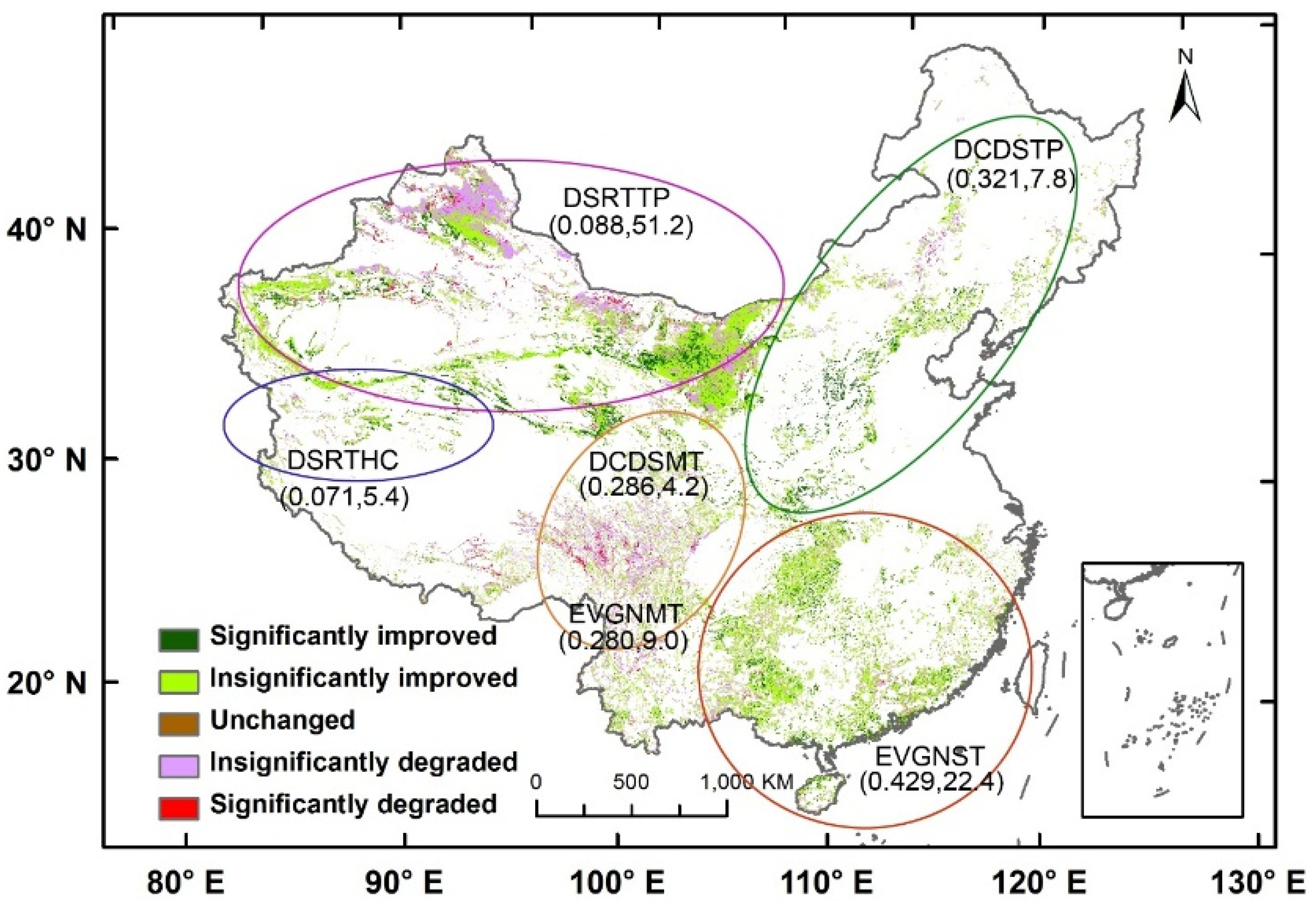
In this paper, we analyzed the spatiotemporal trend of MODIS (Moderate Resolution Imaging Spectroradiometer) EVI (Enhanced Vegetation Index) of six shrubland types in China from 2001 to 2013 and its relationship to intra- and inter-annual regional climate dynamics, which confirmed our hypotheses. The shrublands EVI of China increased significantly from 2001 to 2013 at a rate of 1.01 × 10⁻³ EVI∙a−1. The two main shrubland types (subtropical evergreen and temperate deciduous shrublands) increased at a very high speed of 1.88 and 1.89 × 10⁻³ EVI∙a−1, respectively. In addition, the EVI of two desert shrub types also increased significantly, whereas the subalpine evergreen shrubland EVI decreased significantly. We also detected a lengthened growing season of temperate deciduous shrubland, which partly followed the second hypothesis. The last hypothesis, that regional climate dynamics and growing season length significantly affected the annual averaged shrublands EVI, was also verified. The precipitation variation played a more important role in the EVI variation than temperature, which can be attributed to the water-limited habitat of shrublands.
The increased annual average EVI of the shrublands in China may have significantly enhanced their contribution to the regional ecosystem production and carbon sequestration. The strong increasing trend of EVI for the temperate deciduous shrubland in northern China may point on increasing capacity for their expansion into grasslands, so as the extended growing season to fall that may favor shrublands in competition with the summer-active grassland.


