Article

Daytime Thermal Anisotropy of Urban Neighbourhoods: Morphological Causation

by
E. Scott Krayenhoff
and
James A. Voogt
*
Department of Geography, Western University, London, ON N6A 5C2, Canada
*
Author to whom correspondence should be addressed.
Remote Sens. 2016, 8(2), 108; https://doi.org/10.3390/rs8020108
Submission received: 30 October 2015 / Revised: 6 January 2016 / Accepted: 8 January 2016 / Published: 30 January 2016

Abstract

:
Surface temperature is a key variable in boundary-layer meteorology and is typically acquired by remote observation of emitted thermal radiation. However, the three-dimensional structure of cities complicates matters: uneven solar heating of urban facets produces an “effective anisotropy” of surface thermal emission at the neighbourhood scale. Remotely-sensed urban surface temperature varies with sensor view angle as a consequence. The authors combine a microscale urban surface temperature model with a thermal remote sensing model to predict the effective anisotropy of simplified neighbourhood configurations. The former model provides detailed surface temperature distributions for a range of “urban” forms, and the remote sensing model computes aggregate temperatures for multiple view angles. The combined model’s ability to reproduce observed anisotropy is evaluated against measurements from a neighbourhood in Vancouver, Canada. As in previous modeling studies, anisotropy is underestimated. Addition of moderate coverages of small (sub-facet scale) structure can account for much of the missing anisotropy. Subsequently, over 1900 sensitivity simulations are performed with the model combination, and the dependence of daytime effective thermal anisotropy on diurnal solar path (i.e., latitude and time of day) and blunt neighbourhood form is assessed. The range of effective anisotropy, as well as the maximum difference from nadir-observed brightness temperature, peak for moderate building-height-to-spacing ratios (H/W), and scale with canyon (between-building) area; dispersed high-rise urban forms generate maximum anisotropy. Maximum anisotropy increases with solar elevation and scales with shortwave irradiance. Moreover, it depends linearly on H/W for H/W < 1.25, with a slope that depends on maximum off-nadir sensor angle. Decreasing minimum brightness temperature is primarily responsible for this linear growth of maximum anisotropy. These results allow first order estimation of the minimum effective anisotropy magnitude of urban neighbourhoods as a function of building-height-to-spacing ratio, building plan area density, and shortwave irradiance. Finally, four “local climate zones” are simulated at two latitudes. Removal of neighbourhood street orientation regularity for these zones decreases maximum anisotropy by 3%–31%. Furthermore, thermal and radiative material properties are a weaker predictor of anisotropy than neighbourhood morphology. This study is the first systematic evaluation of effective anisotropy magnitude and causation for urban landscapes.

Graphical Abstract

1. Introduction

Surface-atmosphere exchanges of heat and water are core drivers of the fair-weather meteorology and climatology of cities. Assessment of these energy fluxes is undertaken within the context of the surface energy balance [1], which determines surface temperature, drives atmospheric boundary layer processes and controls thermal climate. Hence, better understanding and measurement of the urban energy balance is required to more effectively adapt our built environments for the purposes of, for example, urban heat mitigation, air pollution dispersal and water management.
Surface temperature is a determining factor for each energy flux in the surface energy balance, with the exception of shortwave radiation. Passive remote sensing of upwelling thermal radiance is an efficient means of observing surface temperature. The protocols and corrections for doing so are well established over relatively flat, undeveloped landscapes [2], but complex three-dimensional (3-D) urban surfaces present additional challenges [3].

1.1. Neighbourhood-Scale Thermal Anisotropy

There are three primary causes of error in the derivation of true (kinetic) surface temperatures from remote sensing of urban areas: (1) atmospheric absorption, emission and scattering between the surface and the sensor; (2) unknown spatial variability of surface emissivity; and (3) for remote sensors with directional or limited fields of view (FOV), sensitivity to micro-scale surface temperature variation due to differences of the effective 3-D radiometric source area (i.e., the instantaneous FOV projected onto the surface) with viewing angle. Atmospheric corrections have received substantial attention, and corrections employing radiative transfer models are reasonably successful [4,5]. Conversely, the latter two causes of uncertainty in remotely-sensed temperature have received comparatively little attention; the third cause in particular results in a directional brightness temperature (TB; [6])—the blackbody temperature corresponding to the radiance actually observed with a radiometer—differing with sensor viewing angle. This effect is fundamentally a product of an urban form combined with a surface temperature variation, rather than a property of the individual surface materials and has been referred to as effective thermal anisotropy [7].
In urban landscapes, as in many natural landscapes, individual surfaces are generally assumed to emit and reflect diffusely, that is, with a radiant intensity (W·rad−1) proportional to cos (Θ), where Θ is the angle from normal [8]. However, the “rough” morphology of these landscapes in combination with variable solar angle results in anisotropic emission and reflection from the surface at larger (e.g., neighbourhood and local) scales, hence “effective” anisotropy. This effect is particularly pronounced during strong solar insolation, which results in variation with viewing angle of the relative proportion of warm sunlit versus cool shaded surfaces “seen” by the sensor. This variation makes interpretation of thermal remote sensing observations problematic, but if anisotropic distributions can be related to quantities such as surface geometry or bulk fluxes it has the potential to be a valuable source of information.

1.2. Observations of Urban Effective Thermal Anisotropy

Effective thermal anisotropy has been observed for a variety of surfaces, namely plant canopies [9,10,11,12], forests [13,14,15], and over larger scale terrain, including the influence of orography [16,17,18,19]. The first remote sensing observations of urban surface temperature were reported by Rao [20]. The importance of research into the effects of anisotropy on thermal remote sensing in urban areas was recognized by Roth et al. [21] in their study of satellite-derived urban temperatures. Since then a few studies reporting anisotropy have been undertaken in urban areas using airborne [7,22,23,24,25,26,27], tower [28,29], as well as combinations of ground and remote measurements [30]. Direct satellite observations of anisotropy over urban areas are lacking; Lagouarde et al. [23] estimate the expected anisotropy for the AVHRR sensor. Voogt and Oke [7], Lagouarde et al. [23] and Lagouarde et al. [26] report observed effective anisotropy of similar magnitude to atmospheric corrections applied to remotely-sensed observations, while Voogt and Oke [3] note that urban areas exhibit strong thermal anisotropy relative to many other landscapes.

1.3. Modelling Urban Effective Thermal Anisotropy

Few case studies of urban effective thermal anisotropy exist, and they each possess a unique combination of surface form and properties, weather conditions, solar angles, sampling angles and sampling fields of view. Sugawara and Takamura [24] use observations and modeling to present the only systematic investigation to date of biased sampling of the TB distribution over urban areas, and they focus on the difference between a limited FOV nadir view and a hemispheric view. In order to isolate individual factors that generate effective anisotropy and to investigate the full range of each factor, the energy balance of individual urban surface facets and neighbourhood-scale sensor viewing of the surface must be modelled. In their review of thermal remote sensing of urban climates, Voogt and Oke [3] identify the coincident use of urban energy balance models and sensor-view models “to better simulate and understand urban thermal anisotropy” as a key area for future research in the field. More recently, Lagouarde and Irvine [25] conclude that urban effective thermal anisotropy is primarily governed by surface geometry, and hence the coincident use of 3-D energy balance and remote sensing models is justified. Moreover, modeling effective thermal anisotropy is important to improve estimation of surface sensible heat flux [31,32] and upward longwave flux [24], and to correct images from large swath satellite data [26]. It may also be useful to isolate the thermal status of individual components of the urban surface [26], to compute aerodynamic properties of urban areas [33], and to composite images from different viewing directions by satellites to construct time series of land surface temperature.
Urban surface temperature distributions that are of relevance to effective thermal anisotropy evolve on a time scale of minutes, and a short lag due to the thermal inertia of the surface is typically observed [26]. Hence, there is little dependence on the surface temperatures prior to the day in question, and simulations need only account for the present day’s energy exchanges. Here, we combine an optimized version of the “Temperatures of Urban Facets in 3-D” (TUF3D; [34]) energy balance model with a modified version of the Surface–sensor–sun Urban Model (SUM; [35]) to investigate effective thermal anisotropy. Both models have been rigorously evaluated and shown to perform well [34,35,36,37], and they have previously been combined [36,38,39]. This model combination permits the evaluation of effective anisotropy for dry, moderately complex urban forms—though relatively simple geometries are chosen here—and it includes sub-facet scale temperature variation at the scale of the chosen model resolution. Voogt [37] finds that sub-facet scale surface temperature variation is an important ingredient in observed anisotropy magnitude. Most previous approaches have used facet-average temperatures with varying degrees of geometrical realism [26,27,38]; Henon et al. [40] are an exception.

1.4. Objectives and Degrees of Freedom

Numerous factors influence urban surface temperature distributions and their viewing by remote sensors, and hence control the magnitude of effective anisotropy of brightness temperature. We distinguish “direct” and “indirect” factors (Figure 1), where the former refer to the temperature distributions and facet-sky (or sensor-facet) view factors that “directly” result in anisotropy, whereas the latter refer to the determinants of the “direct” factors. TUF3D and SUM each determine one direct factor: surface temperature distribution and sensor-facet view factors, respectively. “Indirect” factors affecting the urban surface temperature distribution may be grouped into structural/morphological (gross urban form, size and distribution of small scale elements, regularity), material (thermal and radiative characteristics and their distribution), solar (location, season and local time, or solar angle), and boundary-layer (thermal and dynamical state of the atmosphere) categories. Sensor position and characteristics also influence measured effective anisotropy, but do not affect the anisotropy of emitted thermal radiation.
Urban form is expected to be a strong control on effective anisotropy [7], and at the neighbourhood and local scales it is often more easily characterized (e.g., in terms of building plan area density, λp, and related parameters) than other factors, such as material parameters that often display significant spatial variability. Furthermore, urban form affects both “direct” factors. Therefore, this work focuses on geometric determinants of anisotropy, specifically: λp (building plan area fraction), building aspect ratio (H/L; together, H/L and λp define the canyon aspect ratio H/W), and street orientation (η). Note that H/L is a property of the buildings only; it is their height relative to their length or width. H/W is the more common descriptor in urban climatology: the height of the buildings relative to the spacing between them. Note that H/W as rendered here is strictly only valid for regularly-spaced arrays of square footprint buildings. Though it appears to be a two-dimensional metric of the urban surface, H/W also measures the ratio of wall area to floor (road) area.
Figure 1. Conceptual diagram elaborating the indirect and direct factors that drive and modulate effective thermal anisotropy, and their relatedness. * The only “indirect” factor that affects facet-sky (or sensor-facet) view factors; ** Effective thermal anisotropy is observed by limited fields of view (FOV) sensors, in which case the facet-sky view factor distribution underlies the variation of sensor-facet view factor with sensor view angle.
Remotesensing 08 00108 g001
Modelling is performed for clear skies and low wind speeds (mean of 2.0 m·s−1), atmospheric conditions for which anisotropy is expected to be maximized. Full daytime simulations at summer solstice for six latitudes spanning a range of 50° are simulated, since the diurnal solar path is an important control on anisotropy and interacts strongly with the geometric controls. Effects of material properties on anisotropy are investigated in the penultimate section.
A primary aim of this work is to assess the morphological and solar factors that modulate daytime anisotropy for simplified urban configurations. Another aim is to provide researchers of the urban thermal environment with tools to quickly estimate effective thermal anisotropy for common neighbourhood geometries based on general and accessible scenario descriptors, e.g., solar zenith angle, λp, H/W, and land use. In this spirit, four “local climate zones” [41], ranging from open low-rise (e.g., low density residential) to compact high-rise (e.g., modern North American downtown) are simulated during the summer solstice at two latitudes to explore how effective anisotropy may be expected to vary across a city. Definition and measures of effective thermal anisotropy are briefly discussed next, followed by a description of the modelling approach employed, the results and the conclusions.

2. Defining Effective Thermal Anisotropy

To avoid the difficult issue of temperature-emissivity separation, we investigate the effective anisotropy in terms of TB, the brightness temperature [26]. A good measure of instantaneous effective thermal anisotropy should not be overly sensitive to maximum off-nadir angle (θmax), it should effectively quantify either the average or the maximum difference between two values in the distribution of brightness temperature (TB) observed at different viewing angles, and it should be easy to interpret and calculate from observations (for model-observation comparison purposes). Given the exploratory nature of the present work, identifying the bounds of effective anisotropy (i.e., maximum differences) is the focus.
We define the maximum thermal anisotropy as the range of a TB distribution resulting from a chosen distribution of view directions [39]:
Λ = T B , max T B , min
Λ gives an upper bound to the magnitude of anisotropy. It is a helpful statistic as long as the distribution of TB is continuous and does not exhibit long “tails” at either end, which is the case for the distributions resulting from the present TUF3D-SUM simulations. However, minimum TB can vary substantially at moderate (i.e., ≈45°) off-nadir angle θ, leading Λ to be sensitive to the choice of θmax.
The measure adopted by Voogt and Oke [7] and Lagouarde et al. [26] is based on the use of the nadir temperature as a reference because it is the easiest to define. It is advantageous in an operational sense in that it quantifies the maximum difference from TB,nad (i.e., TB at θ = 0°), which is virtually identical to the mean temperature of horizontal surfaces, or the bird’s eye temperature as defined by Voogt and Oke [31]—the nadir temperature includes a small fraction of vertical surfaces in its FOV. A possible downside of this measure is that, for a given TB distribution, it will vary depending on the magnitude of TB,nad relative to the other values of TB in the distribution (i.e., for an otherwise identical distribution, these measures will differ significantly if TB,nad approximates the minimum or maximum of the distribution versus its mean). Maximum difference from TB,nad is quantified as follows:
ν = max ( T B , max T B , n a d , T B , n a d T B , min )

3. Model Linkage and Evaluation

3.1. Coupling TUF3D and SUM Models

TUF3D is a dry, three-dimensional microscale urban energy balance model with the ability to simulate surface temperatures at the sub-facet scale for a variety of neighbourhood geometries, distributions of surface properties, atmospheric states, and solar angles [34]. All surfaces are plane-parallel, and each urban facet (i.e., roof, street, or wall) is divided into square patches. Radiative, conductive, and convective energy exchanges are modeled at each patch, the balance of which determines the change in patch surface temperature at each time step. Radiative exchange is modeled for shortwave (≈0.2–3.5 μm) and longwave (≈3.5–100 μm)) bands, and all radiation emission and reflection is assumed to be Lambertian. Direct shortwave irradiance and inter-patch visibility are determined with ray tracing, and exchanges (e.g., multiple reflections) between all patches in both wavebands use view factors determined analytically. The radiative exchange module has finer (sub-facet) spatial resolution and has been more thoroughly evaluated than the convective module; as such, TUF3D implicitly assumes that radiative exchange is the primary control on microscale surface temperature variation. Modelled surface temperatures perform well against full-scale urban surface temperature observations at both facet and sub-facet scales [34].
All TUF3D domains used in the present work are composed of repeated “urban units”, which consist of one building or block surrounded by road. In the optimized version of TUF3D, an urban unit is defined as the smallest plan area that encompasses all of the domain’s morphological variation and repeats throughout the domain [34]; repeated urban units provide radiative boundary conditions for the central urban unit. TUF3D surface temperatures from the central urban unit are replicated over an N by N array by the modified SUM model to provide an urban surface of sufficient size for viewing by the remote sensor with specified height, view angle, and FOV, where N is the number of urban units (Figure 2). SUM then views the surface over the specific range of off-nadir (θ) and azimuthal angles (ϕ).
Figure 2. A schematic of a sensor at height ZS viewing a limited domain composed of regular “urban units”. θmax = maximum off-nadir viewing angle; FOV = sensor field of view.
Remotesensing 08 00108 g002
Each patch is split into four square sub-patches for greater sensor-viewing accuracy. The sensor-to-surface view factor for each sub-patch k of patch i that is seen by the sensor (ψsens,i,k) is calculated using contour integration [42]. The sensor is approximated as an infinitesimal area and the sub-patch as a finite area. The apparent surface temperature as viewed by the sensor is then determined using the Stefan-Boltzmann relation (i.e., a broadband approximation):
T B ( θ , ϕ ) = [ i = 1 n k = 1 4 [ ( ε i σ T s f c , i 4 + ( 1 ε i ) L i ) ψ s e n s , i , k ] | S s ( θ , ϕ ) σ i = 1 n k = 1 4 ψ s e n s , i , k | S s ( θ , ϕ ) ] 1 4
where TB is the apparent (brightness) temperature of the surface viewed with sensor off-nadir angle (θ) and sensor azimuthal view angle (ϕ), Tsfc,i and L i are the TUF3D kinetic surface temperature of patch i and total incident longwave radiative flux density on patch i after multiple reflections, respectively, n is the number of patches in the domain, k is an index referring to the sub-patch, and Ss(θ,ϕ) indicates only sub-patches seen by the sensor for view angles θ and ϕ. Sub-patch temperature and incident longwave are both equal to their corresponding values for the whole patch. Lagouarde et al. [26] show that the broadband approximation is sufficiently accurate for the present purposes.

3.2. Sampling the TB Distribution

There are many view angles from which to choose in sampling a surface with a remote sensor. For example, the specific set of θ and ϕ combinations may be chosen at random, at regular intervals of θ and ϕ, or such that each sample is representative of an equal solid angle subdividing a hemispherical FOV sensor such as a pyrgeometer. Here we sample at regular intervals of both θ and ϕ, because it is simpler and also sufficient to capture the range of TB. Statistics describing the average or most probable difference in a remotely-sensed distribution would require weighted random sampling. The modeled remote sensor is positioned at a sufficient height such that it samples a representative portion of the N by N surface array (Section 3.1) while minimizing computation time.
Simulations are performed to determine the resolution required to accurately represent a facet (i.e., roof, wall, or street) in TUF3D and SUM, which employ the same resolution. SUM is implemented here to view the intra-facet temperature variation, whereas all previous applications with the exception of Voogt [37] have been limited to sunlit and shaded facet-scale average temperature inputs from either direct observation or facet-averaged energy balance models such as that of Mills [38,43]. Krayenhoff and Voogt [34] suggest that TUF3D should be run with a minimum of four patches across any facet, while Krayenhoff [36] finds that modelled anisotropy at a resolution of four is sufficiently similar to that obtained with a resolution of ten. Thus, a minimum resolution of four patches across any facet is chosen for computational efficiency. However, the division of patches into sub-patches for SUM viewing results in an effective resolution of eight. TUF3D-SUM tests for limited ranges of surface geometry and atmospheric forcing indicate that use of facet-average sunlit and shaded temperatures causes SUM to underpredict anisotropy (relative to that with the full sub-facet surface temperature variation) by ≈10%, by underpredicting TB,min less than TB,max (not shown).

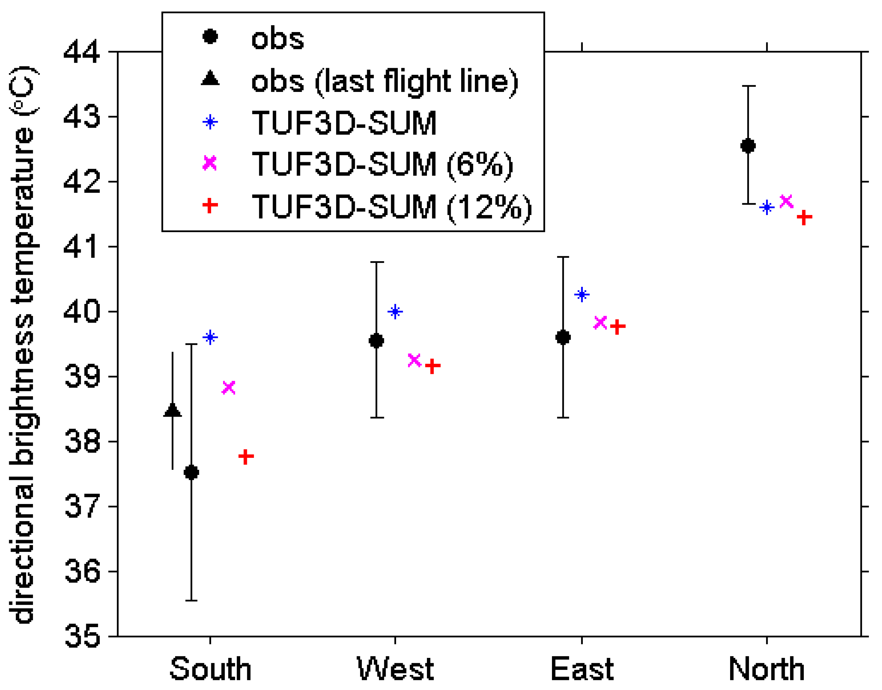
3.3. Model Evaluation: Vancouver Light Industrial Site

As discussed in Section 1.3, TUF3D and SUM have each individually been evaluated against appropriate datasets. Nevertheless, it is prudent to evaluate their combined ability to model directional viewing of urban surface temperature and to produce effective thermal anisotropy. Airborne thermal scanner observations taken 15 August 1992 in the “Vancouver Light Industrial” neighbourhood are chosen for model evaluation [7,32]. While the TUF3D-SUM combination is ultimately intended to inform satellite thermal remote sensing in particular, airborne observations are chosen for the present model evaluation for several reasons: (1) Five view angles are available vs. one view angle for typical satellite observations; (2) The scale of the measured area (i.e., sensor FOV) is small enough to avoid variability due to topography, land-cover variation, etc.; (3) Tower observations of air temperature, wind speed, and humidity required by TUF3D are available.
The Vancouver Light Industrial neighbourhood was characterized by rectangular-footprint buildings of 1–3 storeys, flat roofs, and little vegetation (<5% plan area). Airborne observations of surface temperature were acquired during three daytime flights, and the midday period (flight 2; 1235–1320 Local Solar Time) is chosen here. Directional (brightness) radiometric surface temperature was acquired by a 12° FOV sensor at five view directions: nadir, and in each of the cardinal directions with 45° off-nadir angle (θ). Tower measurements of meteorological variables were conducted concurrently, providing forcing data for TUF3D.
A 48-h TUF3D simulation is conducted starting at 0000 LST 14 August 1992, to provide ample time for the model to adjust to the atmospheric forcing. An optimized version of TUF3D is used: regular arrays of square-footprint buildings with appropriate neighbourhood-average characteristics are modelled instead of using a more precise rendering of the neighbourhood, as in Voogt [37]. TUF3D input parameters are those in Krayenhoff and Voogt [34] and Masson et al. [44], with one primary adjustment. Due to a combination of sustained winds (sea breeze), large roof area (λP = 0.51), and low measurement height (z ≈ 1.5 H) [meaning that forcing data may not represent the neighbourhood average], directional brightness temperature is sensitive to parameters that modulate roof sensible heat flux and therefore roof temperature (which is challenging to reproduce for this scenario [44]). Hence, the most uncertain such parameter, roof roughness length, is reduced from 0.15 m in Krayenhoff and Voogt [34] and Masson et al. [44] to 0.005 m here, to adjust the roof temperature and therefore the overall magnitude of directional brightness temperature. This corresponds to an average obstacle size on the predominantly flat roofs of the order of 0.05 m, which is not unreasonable. Moreover, this modification is likely a surrogate for the uncertain yet impactful ratio between roughness lengths for momentum and heat [32]. Recall that it is the ability of TUF3D-SUM to reproduce differences between directional temperatures that is of importance here; absolute temperatures remain challenging for most urban canopy models due to parameter uncertainties in complex urban environments, insufficient or inadequate data for evaluation of model components (especially convection modules), among other factors.
TUF3D output brightness surface temperatures are extracted for all patches in the central urban unit at 1300 LST 15 August 1992, for viewing by SUM. SUM temperature at an off-nadir angle of θ = 45° in each of the cardinal view directions is then compared to the median of all images taken in each view direction during the flight (Figure 3). Modelled temperature is at the low end of the observed range in the North (warm) view direction, and at the high end of the observed range in the South (cool) view direction. Modelled temperatures are well within the range of observed variation for the East and West view directions. Most importantly, for our purposes, the model tends to underestimate the range of temperature variation (between the North and South view directions), calculating a value of 2.0 K compared to the 5.0 K that is observed. A tendency for models to underestimate observed anisotropy has been noted before [26,38,45]. Voogt [37] found that detailed surface structure and microscale temperature variability were both important to capture the full anisotropy magnitude. Henon et al. [40] investigated the contribution of sub-facet temperature variability to anisotropy compared to homogeneous facet temperature.
Figure 3. Directional sensor apparent (brightness) temperature of the Vancouver Light Industrial neighbourhood at ≈1300 LST 15 August 1992, for four view directions at an off-nadir view angle of 45°. Observed (obs) temperature median and interquartile range of all images during the flight are shown, as well as “Temperatures of Urban Facets in 3-D” (TUF3D)-Surface–sensor–sun Urban Model (SUM) temperature with and without small scale structure (6% and 12% refer to the plan area coverage of small scale structures).
Remotesensing 08 00108 g003
TUF3D-SUM has the capacity to include microscale (sub-facet scale) surface temperature variation. However, its surface temperature distribution is driven primarily by (shortwave) radiation exchange, and by the surface structure that modulates this exchange. The results in Figure 3 arise from a highly simplified surface structure, devoid of structures smaller than buildings such as cars, hedges, fences, poles, signs, bus shelters, chimneys and other rooftop structures, etc. Hence, two tests are performed to examine the effects of ignoring these smaller structures (Figure 3): one cubic cell of 1.45 m on a side (i.e., the size of a patch in TUF3D) is introduced at regular intervals on all roads and roofs with plan area coverage of 0.06; two contiguous such cells, aligned in the east-west direction, are introduced for a plan area coverage of 0.12. These additions enhance both the detail of the surface structure, and as a consequence, the microscale temperature variability. They do not affect the North (warm sunlit) view direction, but substantially reduce the temperature in the South view direction, by ≈1 K and ≈ 2 K, respectively, and the East and West view directions to a lesser extent (Figure 3). Essentially, these two additions of small scale (sub-facet scale) structure generate more shaded area, reducing the South view temperatures and increasing the anisotropy to 2.9 K and 3.7 K, respectively.
Another potential cause of the model’s underestimation of anisotropy magnitude and overestimation of South facing temperature derives from variability in the observations themselves. Flight 2 is composed of three flight lines, each under 60 s in length, and about 6–7 min apart. During the 13 min between the first and third flight line, the median temperature of the South view increases by 3.5 K, which represents 70% of the observed anisotropy magnitude; this suggests that either neighbourhood surface temperature variability is noteworthy and spatial sampling differs between the flight lines, or that portions of the surface within the South FOV are heating up rapidly. Neither of these variabilities are represented in the TUF3D-SUM results in Figure 3; however, if the last flight line is plotted on its own, the South view radiometric temperature increases by 0.9 K (Figure 3) and the North view by only 0.1 K (not shown), decreasing observed median anisotropy by 0.8 K to 4.2 K.
This evaluation suggests that TUF3D-SUM captures the qualitative variation of directional brightness temperature between the four off-nadir view directions tested. However, the full forcing for anisotropy appears to be underrepresented, at least without the addition of small scale structure. Addition of sufficient small scale structure raises modeled anisotropy magnitude to approximately 70%–80% of that observed, or to 90% of the anisotropy of the last set of flight lines; however, the area of small scale structure introduced, though not excessive, was not based on a measurement of the actual amount present in the neighbourhood. Moreover, directional brightness temperature is sensitive to certain parameters in TUF3D for this particular scenario. Therefore, we proceed with model sensitivity experiments of arrays of square-footprint buildings without small scale structure, with the caveat that they likely underestimate anisotropy relative to most real neighbourhoods. In essence, we aim to capture the variation of the contribution to total anisotropy magnitude that is produced by the blunt, simplified building structures.

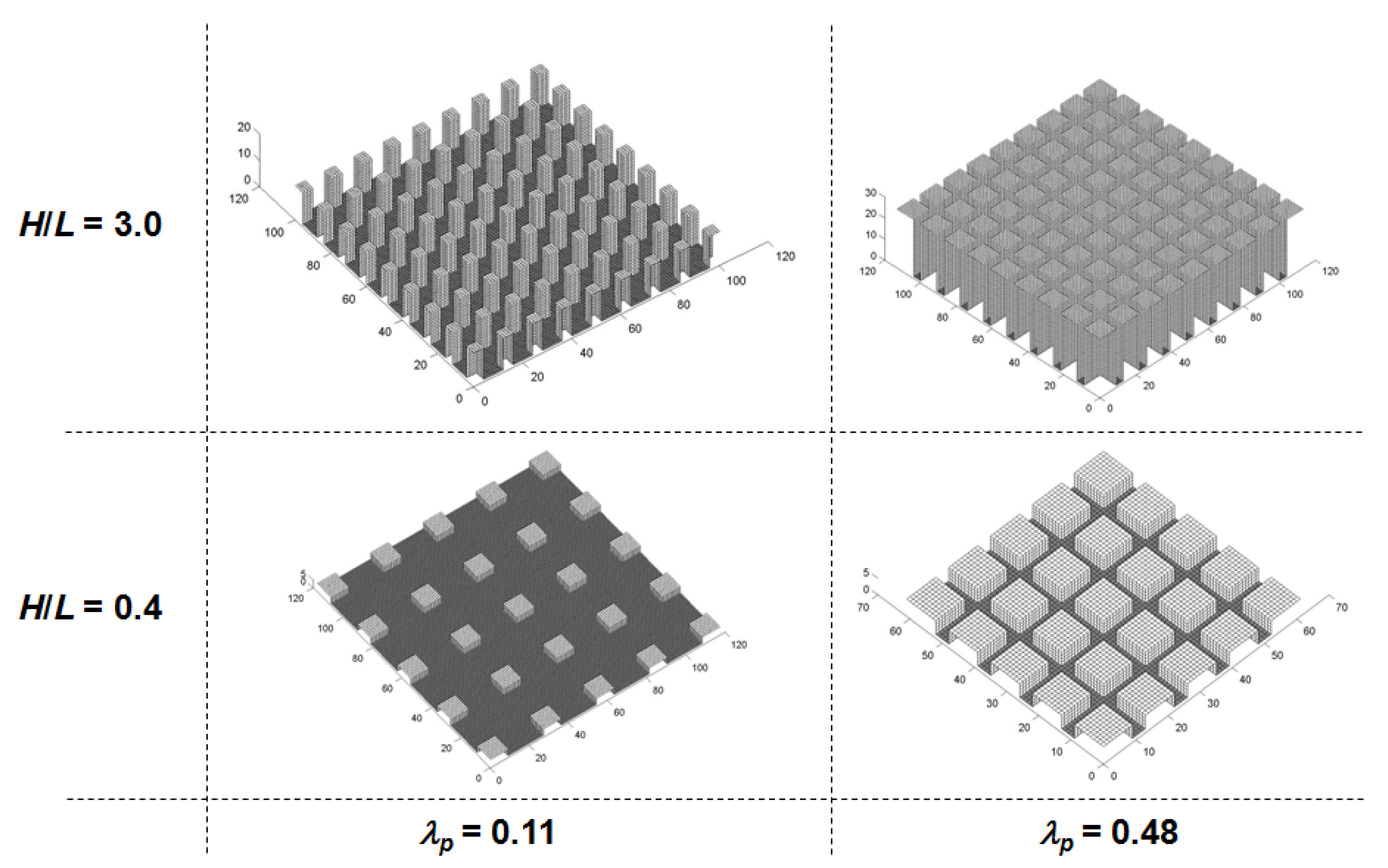
4. Effects of Urban Geometry on Anisotropy: Simulation Design

Full-day TUF3D-SUM simulations are performed for a range of latitudes and simple cubic array geometries. In the terms introduced in Figure 1, structural and solar parameters are varied, while boundary-layer and material parameters are held constant (and the latter are additionally assessed in Section 6.2). TUF3D simulations use urban atmospheric forcing (air temperature, wind speed) measured at 31.8 m on 21 June 2002 at the Basel Sperrstrasse site (47°34′N, 7°35′E) during the BUBBLE experiment [46]. Latitudes of 20°, 30°, 40°, 50°, 60°, and 70° are simulated for 21 June increasing the range of solar paths sampled. K d i r , K d i f and L are calculated by TUF3D internal routines assuming clear skies [47,48,49].

Arrays of Buildings with Square Footprints

A suite of 1944 simulations is performed for June 21 with TUF3D, encompassing all combinations of the increments of building plan area fraction (λp), building height-to-length ratio (H/L), street orientation (η), and latitude. Each simulation is 24 h long. SUM is then run for every daylight hour, on the hour (in local solar time, or LST). η takes values of 0° through 75° in 15° increments, effectively sampling the full range of street orientation due to the symmetry of the urban surface, while λp takes values spanning the full range of typical urban variation, with approximate values (sometimes adjusted slightly to fit the discrete TUF3D-SUM geometry): 0.06, 0.11, 0.20, 0.25, 0.31, 0.36, 0.41, 0.48 and 0.54, and H/L takes on the following approximate values for each λp: 0.4, 0.7, 1.0, 1.5, 2.0, 3.0. In Figure 4, the approximate range of variation of λp and H/L are visualized in the TUF3D domain; the more unrealistic geometries considered are the highest H/L geometries, in particular when combined with high λp. The variables λp, H/L and η together fully describe the variation of regularly-spaced, aligned arrays of identical square-footprint buildings. Radiative and thermal parameters are those for Basel Sperrstrasse in Krayenhoff and Voogt [34].
Trees, sloped roofs, poles, balconies, chimneys, hedges, cars, pedestrians, benches, bins, and other common structural components of urban neighbourhoods are all ignored. While they each undoubtedly contribute to anisotropy for a certain range of scenarios, the assumption is that the blunt building shapes provide the majority of the anisotropy in most cases. Lagouarde et al. [26] find that roof slope only modestly affects anisotropy, while Voogt [37] show that addition of roof structures have very modest impact, for example. Regardless, this is the simplifying assumption in the present work, and it is a first step toward meaningful exploration of urban effective anisotropy.
Figure 4. Example TUF3D domains for two λp and H/L ratios, showing (approximately) the range of geometries considered.
Remotesensing 08 00108 g004

5. Effects of Urban Geometry on Anisotropy: Results and Discussion

The TUF3D-SUM models as presently applied produce angular distributions of remotely-sensed apparent temperature for arrays of simplified buildings. For example, in Figure 5, 1200 LST results for two neighbourhoods at three street orientations are shown. The neighbourhood with lowrise buildings (H/L = 0.4) exhibits the classic “hot spot” observed in several studies [23,26], and the hot spot shifts clockwise and fades slightly with the rotation of street orientation. The hot spot location also suggests a lag relative to the solar azimuth angle, in particular for η = 0°, driven by thermal inertia of the surface.
Figure 5. Example polar plots of TUF3D-SUM simulated effective anisotropy, for two neighbourhood geometries (top row: λP = 0.32, H/L = 0.4, H/W = 0.6; bottom row: λP = 0.31, H/L = 1.6, H/W = 2.0) and three street directions, at 1200 LST 21 June at a latitude of 60° (solar zenith angle = 36.5°). Concentric circles are, from center, off-nadir angles of 5°, 15°, 25°, 35°, and 45°. Labelled radial lines refer to azimuthal angle. The vertex of the black, bold “<” indicates the position of the sun.
Remotesensing 08 00108 g005
A neighbourhood with similar density (λP = 0.25) but much taller buildings (H/L = 1.6) exhibits two hot spots (Figure 5), which so far has not been observed to the authors’ knowledge. The secondary hot spot (below nadir on the plot) arises from increased viewing of hot roofs and reduced viewing of shaded streets, which more than offset increased viewing of shaded north-facing walls, as sensor off-nadir angle increases from nadir with azimuthal view angle toward the sun. These hot spots also change in magnitude and location as the street orientation shifts clockwise. Also note the detail in these plots that is not produced by previous modeling approaches [26], likely because the current approach uses 3-D geometries and the associated microscale surface temperature distributions from TUF3D.

5.1. Variation of Anisotropy With Neighbourhood Geometric Structure

Anisotropy varies with neighbourhood geometry and the angle of incidence (relative to neighbourhood layout) and flux density of shortwave radiation. It is helpful to first visualize this variation for select scenarios before proceeding to general patterns and relations.
In Figure 6, variation of maximum anisotropy (Λ) and maximum difference from nadir (ν) are plotted as a function of building plan area fraction (λP) and building height-to-length ratio (H/L), for two latitudes at 1200 LST (i.e., for two solar zenith angles). Λ and ν exceed 11 K for specific geometries when the sun is near zenith, and exceed 5 K when it is at a more moderate elevation of 53.4° above the horizon. Both measures of anisotropy peak for moderate densities of tall buildings, especially for smaller solar zenith angle. Maximum anisotropy is 9% larger than ν for the small solar zenith angle (6.5°), in the median, and 39% larger for the larger solar zenith angle (36.6°).
There are three stages of variation with respect to H/W apparent in Figure 6 (and Figure 7 below), for both Λ and ν: anisotropy increases concurrently with H/W for all scenarios until H/W ≈ 1.0–1.5; from that point up to H/W ≈ 3.0–4.0 anisotropy peaks, and demonstrates large variation between neighbourhoods within this H/W range; and finally, relatively constant anisotropy for even larger H/W. In the middle stage, moderate densities of tall buildings generate higher anisotropy than those with high densities of buildings of modest relative height H/L. Most real urban neighbourhoods exhibit H/W ≤ 1.5, i.e., in the linear range [50]. Note that variable roof heights are possible in both TUF3D and SUM, but are not investigated in the present work so as to focus on other aspects of the urban geometry.
Figure 6. Maximum anisotropy (left) and maximum difference from nadir (right) as a function of geometric ratios H/L and λP, for 1200 LST 21 June at latitudes 30° (a,b) and 60° (c,d). Values are averaged over all street orientations. Dashed, numbered lines are building height to street width ratios (H/W).
Remotesensing 08 00108 g006
Figure 7. Maximum anisotropy as a function of building height to street width ratio H/W for all latitudes and hours 1200–2000 LST (inclusive) on 21 June. Values are averaged over all street orientations.
Remotesensing 08 00108 g007
Overall, these results suggest H/W is a more useful predictor of anisotropy than either λP and H/L, and it combines both measures to an extent. Moreover, it is a better predictor of anisotropy than any 3-D measure tested, such as the complete-to-plan area ratio (λC). While not shown in Figure 6, the general pattern with H/W is apparent at 1200 LST for most latitudes and times (i.e., all solar zenith angles) sampled, but is most apparent for small solar zenith angle.

5.2. Geometric Causation of Anisotropy

The relation between anisotropy and H/W for different solar elevations is assessed for all latitudes sampled and for a broad range of daylight hours. Solar zenith angle is a function of latitude and time of day in local solar time (and season, which is not investigated here), and is a more direct driver of anisotropy than the latter two quantities. Therefore, simulation results are described and plotted in terms of the solar zenith angle instead of latitude and time of day in the subsequent analysis.

5.2.1. Anisotropy as a Function of Canopy Height-to-Width Ratio

Maximum anisotropy (Λ) as a function of H/W for all daylight hours in the second half of the day (1200–2000 LST, inclusive), binned in 15° increments of solar zenith angle, is plotted (Figure 7). Patterns for the first half of the day are very similar and are not included for clarity. Magnitude of anisotropy increases with decreasing solar zenith angle (i.e., with greater solar elevation and irradiance), as does the slope of the approximately linear increase in Λ for low H/W—increasing building height relative to street width creates more shade, which generates larger temperature differences with greater directional solar irradiance. For moderate H/W (≈1.5–4.0), anisotropy variability appears to increase and create a more pronounced peak; however, the variability of anisotropy between neighbourhoods at a given H/W scales approximately with average neighbourhood anisotropy magnitude up to H/W ≈ 2 (depending on solar zenith).
Patterns in Figure 7 are almost identical for ν (not shown), with two major differences: median magnitude in the solar zenith angle bins is lower by 8%–33% (generally a lower magnitude for larger solar zenith angle), and the peak at moderate H/W is less pronounced for solar zenith angles > 30° (not shown). Lowest values of ν/Λ appear when neither TB,max nor TB,min closely approximate TB,nad, which occurs for H/W > 3.0 for solar zenith angles < 30° [39], and for H/W < 4.0 and solar zenith angles > 30°. In the former cases, TB,maxTB,nad for smaller H/W but diverges for larger H/W as roads receive less shortwave flux, whereas for solar zenith angles >30°, TB,minTB,nad for larger H/W but greater solar penetration to road surfaces for smaller H/W increases TB,nad.

5.2.2. Normalization of Anisotropy Magnitude

A simple normalization permits the collapse of all data in Figure 7 into one plot (Figure 8). Roofs contribute little to anisotropy magnitude in these simulations because all buildings are the same height in the present simulations. Moreover, anisotropy clearly scales with K↓. Hence, Λ and ν, divided by K↓ and (1 − λP), are plotted for all hours (1200–2000 LST) and latitudes (i.e., all solar zenith angles) as a function of H/W (Figure 8). These “normalizations” describe an efficiency of anisotropy production in Km2·W−1, and they collapse the data such that relations become apparent. For clarity, median and interquartile range of normalized Λ and ν are plotted instead of all data.
A linear correlation between H/W and anisotropy remains strong up to H/W ≈ 1.25, which includes many urban neighbourhoods worldwide; primary exceptions are North American-style downtown neighbourhoods, which exhibit densely-packed tall buildings, and the densely-packed, lightly-constructed neighbourhoods that are widespread in economically-disadvantaged areas of the Global South. Linear relations for H/W ≤ 1.25 are:
Λ = a Λ K ( 1 λ p ) H / W
ν = a ν K ( 1 λ p ) H / W
where aΛ = 0.011 Km2·W−1 and aν = 0.008 Km2·W−1. Thus, the relations derived here may be used to assess approximate values of Λ and ν, provided good estimates of neighbourhood-average H/W and λP, and K↓, are available. These relations are derived for simplified urban surfaces with the assumption that geometric and solar forcing are the primary factors that control effective anisotropy. Small scale structural features probably also play a substantial role in real neighbourhoods (e.g., Section 3.3), as do variable building heights, variable radiative and thermal parameters, particular street directions with respect to the sun, etc. Therefore, these relations are better understood as referring to estimates of minimum anisotropy magnitude of real neighbourhoods.
Relatively constant anisotropy is apparent for H/W = 1.25–4.0, with median values over this range of:
Λ = c Λ K ( 1 λ p )
ν = c ν K ( 1 λ p )
where cΛ = 0.014 Km2·W−1 and cν = 0.010 Km2·W−1. For both Λ and ν, the intersection between the linear relation (Equation (4)) and the constant value (Equation (5)) occurs at H/W ≈ 1.25. These relations must be further tested with data from real neighbourhoods; in particular, it should first be determined if H/W (or a similar measure such as the complete-to-plan area ratio) is a good predictor of anisotropy magnitude for real cities, knowing that these relations are likely to predict a minimum magnitude of anisotropy (see Section 3.3). Moreover, the constants aΛ, aν, cΛ and cν in Equations (4) and (5) depend on off-nadir angle (see Section 5.3 below). Notably, Figure 8 suggests that the urban canopy (i.e., the canyon area) becomes even more efficient at producing anisotropy as H/W increases beyond 4.0 (Figure 8).
Figure 8. Maximum anisotropy (a) and maximum difference from nadir (b), both divided by forcing shortwave radiation (K↓) and canopy area (1 − λP), as a function of canyon height-to-width ratio. Median values with interquartile range (error bars) are plotted for each H/W. Slopes of best fit lines for H/W ≤ 1.25 (in red) are 0.011 and 0.008, respectively, with R2 values of 0.93 and 0.94, respectively. Constant values (dashed horizontal red lines) for 1.25 < H/W < 4.0 are 0.014 and 0.010, respectively.
Remotesensing 08 00108 g008
Finally, TUF3D roof surface temperature provides a dimensionally-simple normalization of Λ and ν in place of K↓, and one that collapses the data similarly (i.e., with a linear relation for H/W < 1.25, and constant value for 1.25 ≤ H/W < 4.0), and with a superior fit to K↓ (R2 = 0.98 vs. R2 of 0.93 with K↓, for Λ). However, roof surface temperature depends on roof thermal and radiative parameters, as well as rooftop structures and height variability, whereas K↓ is in this sense of greater utility because it is independent of the surface and furthermore, is easily measured and modeled.

5.2.3. Facets Contributing to Anisotropy

Parameterization of anisotropy as a function of H/W, K↓, and λP offers only limited insight into its causation. Due to the uniform roof height in the present suite of scenarios, anisotropy magnitude is primarily caused by roads and walls, and the relative amounts of sunlit vs. shaded portions of each that are seen by the sensor. Maximum anisotropy (Λ) results from the difference between TB,max and TB,min. The view angle at which TB,max is observed closely corresponds to the solar angle, and so mostly sunlit portions of facets are viewed (i.e., the “hot spot”). Hence, all other factors being equal, TB,max is unlikely to change radically with neighbourhood geometry, and it changes predictably with solar zenith angle: larger solar zenith angle yields a smaller solar flux at the neighbourhood scale and lower anisotropy. On average, the variation of TB,min with H/W for a given solar angle range and H/W < 1.25 is about twice that of TB,max. Therefore, variation of maximum anisotropy (and ν in many cases) with H/W depends more strongly on variation of TB,min than of TB,max.
For small solar zenith angles, Λ grows linearly with H/W because of the rapid increase in sensor view fraction of cool, shaded walls at the TB,min view angle (Figure 9). This is a principal cause of the linear growth in anisotropy in Figure 7 and Figure 8. Walls occupy little of the FOV at the TB,max view angle, conversely, because the solar rays are nearly parallel to the walls whereas they are almost normal to the roads, which are therefore warmer and contribute more to TB,max. For H/W < 1.5 at solar zenith angles ≥ 45°, walls are seen approximately equally at both TB,min and TB,max view angles; shaded walls remain important to TB,min as before, and sunlit walls are now a more important component of TB,max because they are more sunlit, and because roads are more shaded on average at this solar zenith angle.
As H/W increases to ≈2.0–3.0, shaded walls remain more important for TB,min than sunlit walls for TB,max, and conversely, roads factor more significantly at the TB,max view angle than at the TB,min view angle. As H/W increases beyond 3.0, shaded walls remain important for TB,min at low solar zenith angle. At larger zenith angles, road contributes more to TB,min than walls, and walls contribute more to TB,max than roads, because shortwave radiation mostly impinges on walls and does not penetrate deeply into the dense canopy (e.g., to the roads). At larger H/W, the view factor of roofs occupies a larger fraction of the overall sensor view factor; for the range of H/L and λP ratios sampled here, neighbourhoods with higher H/W tend to have higher λP, particularly since the maximum building height-to-length ratio H/L sampled is 3.0.
Figure 9. Total view factor from SUM sensor to roads and walls for TB,max and TB,min view angles as a function of H/W for six solar zenith angle ranges (data from all latitudes and all hours between 1200 LST and 2000 LST, inclusive). Median (symbols) and interquartile range (error bars) for each value of H/W are plotted for clarity.
Remotesensing 08 00108 g009
Overall, shaded (cool) walls are critical to TB,min and therefore to the production of anisotropy, except for more extreme built geometries (H/W > 4.0) combined with low solar elevation angle. In the latter cases, the TB,min view angle approaches nadir and cool road surfaces are more important. TB,max generally changes less with H/W than TB,min, and in that sense its variation is less important to the production of anisotropy. The TB,max view angle closely corresponds to the nadir view angle for small solar zenith angles and small H/W, but diverges otherwise. Thus, the sensor view associated with TB,max is dominated by roads (and roofs) until the combination of higher canopy H/W and lower solar elevation shifts the predominant warmth of the urban canopy to walls.

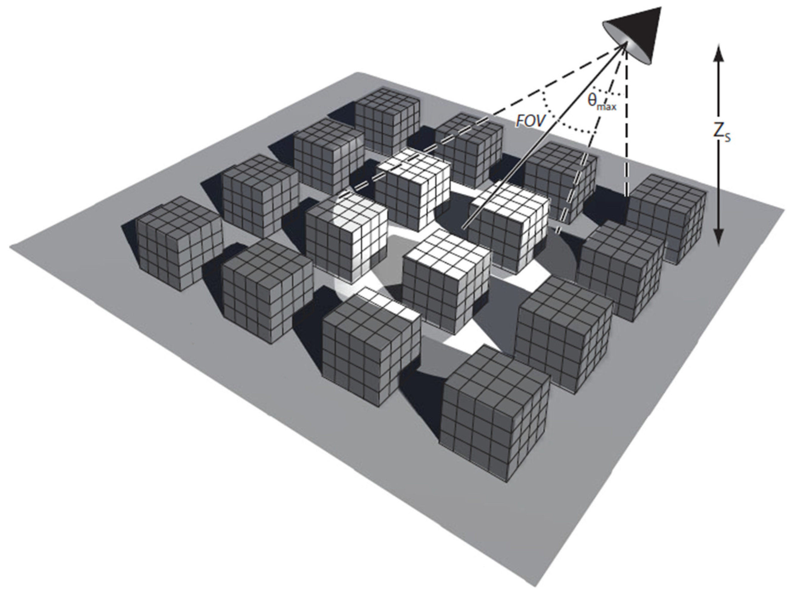
5.3. Sampling Anisotropic Distributions: Maximum Off-Nadir Angle

Results in Section 5.1 and Section 5.2 are based on the maximum difference between any two brightness temperatures, Λ = TB,maxTB,min, or the maximum difference of any brightness temperature from the nadir brightness temperature, ν = max (TB,maxTB,nad, TB,nadTB,min). Results in those sections depend on the maximum off-nadir angle (θmax) chosen, 45°, an angle that approximates the common useable limit of satellite viewing angles (otherwise atmospheric effects and the projected sensor FOV become too large).
To illustrate this effect, the mean difference from TB,nad is plotted as a function of different sensor off-nadir angle (Figure 10). For solar zenith angle < 45° and H/W < 1.25, the slope of increase with H/W varies with off-nadir angle (θ); as expected, greater variation from nadir corresponds to a larger range of θ sampled. For larger solar zenith angle, a muted version of the same variation with off-nadir angle is found. For larger H/W, the reverse variation with θ is found for some solar zenith angles. The important point is that the degree of anisotropy observed depends on the range of off-nadir angles sampled. A possible method that avoids this difficulty is that of Huang et al. [51], who simply compute the mean and standard deviation of the difference between TB(θ) and TB(0°) = TB,nad; however, whether mean and standard deviation are appropriate measures for these distributions is questionable.
Figure 10. Mean temperature difference from nadir view as a function of H/W for three off-nadir angles (ONA), over four solar zenith angle ranges. Model output is for 1200 LST and 1800 LST for all latitudes.
Remotesensing 08 00108 g010

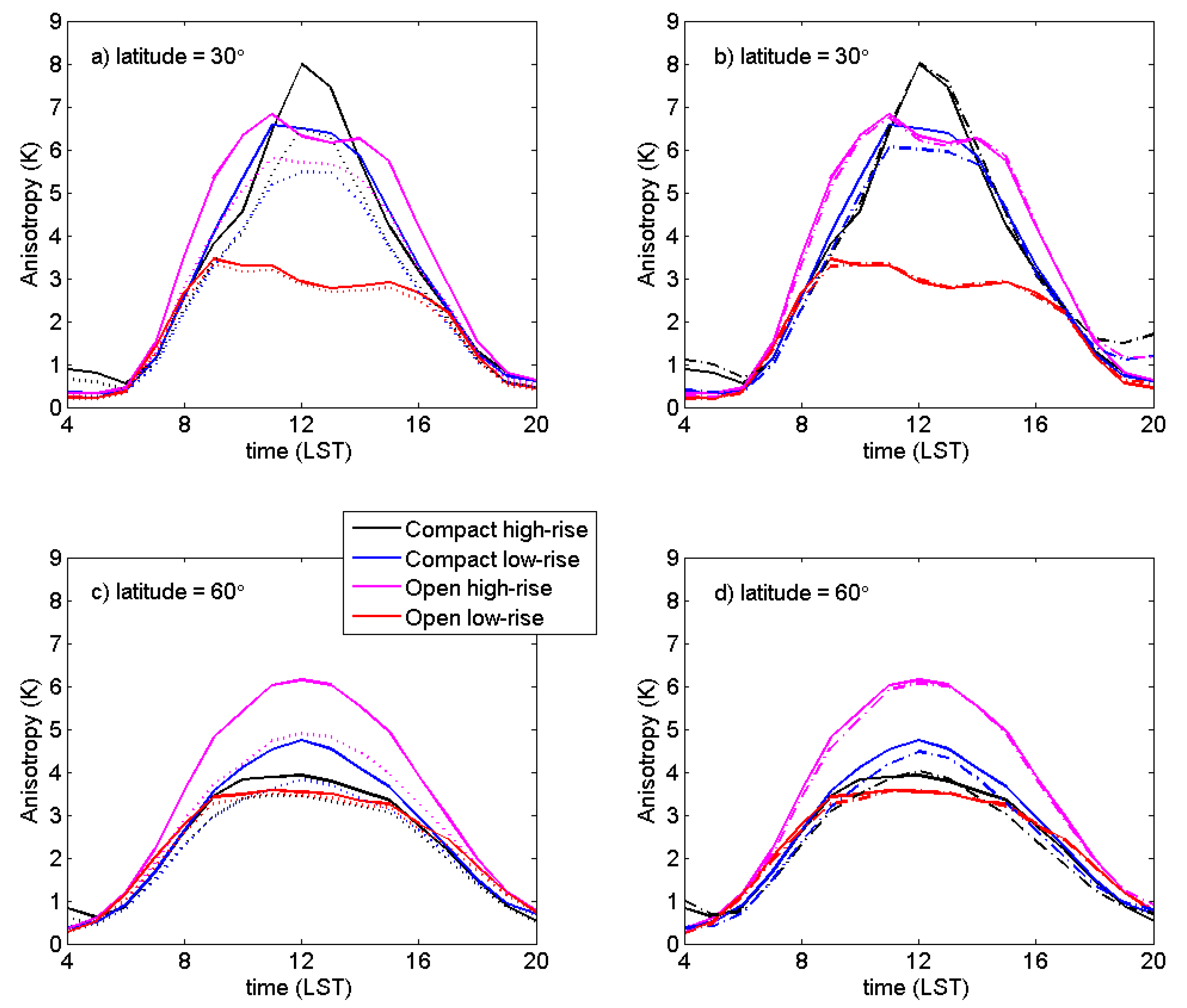
6. Anisotropy of Common Neighbourhoods: Local Climate Zones

Previous simulations of anisotropy of urban zones clearly distinguish between tall commercial zones and shorter residential and light industrial zones [39]. Here, select “local climate zones” (LCZs) [41] with a range of geometries are modeled with TUF3D and SUM: LCZ1—Compact high-rise, LCZ3—Compact low-rise, LCZ4 – Open high-rise, LCZ6 – Open low-rise. The height-to-width ratios for these zones, as modeled here, are H/W = 2.5, 1.3, 1.0, and 0.5, respectively. Input parameters are from Stewart et al. [52]. Modelling is performed for latitudes of 30° and 60° on 21 June. Anthropogenic heat is added as in Krayenhoff and Voogt [53], because it can substantially affect surface temperatures, especially in high density zones such as LCZ1.
Maximum anisotropy varies between latitudes, and it varies between high-rise and low-rise zones in a similar manner to previous work [39]. At a latitude of 60°, variation of anisotropy is smooth and mimics the shape of the incoming solar radiation curve. The “open high-rise” zone generates about 2 K more maximum anisotropy than the other three zones throughout the midday period (Figure 11). The “compact highrise” zone exhibits similar anisotropy magnitude to the two lowrise zones, suggesting that increased λP attenuates anisotropy (e.g., Section 5.2.2). Conversely, at a latitude of 30°, the “compact high-rise” zone produces 1–2 K more anisotropy than the “open high-rise” and “compact low-rise” zones at midday, when its roads are sunlit; however, the “open high-rise” zone exhibits higher anisotropy in the morning and afternoon. The “open low-rise” zone generates about half of the anisotropy magnitude of the other three compact/high-rise zones throughout the midday period for this latitude, probably due to its lower H/W (Section 5.2.2). Maximum anisotropy magnitude is higher and more differentiated between the zones for smaller solar zenith angle (latitude = 30°), except the “open low-rise” zone, for which it is similar for both latitudes.
Figure 11. Diurnal evolution of TUF3D-SUM predicted maximum anisotropy (Λ) for four Local Climate Zones on 21 June. Solid lines indicate default material properties for each zone and the average of the anisotropy for each street orientation (i.e., full regularity of street orientation). (a) Latitude = 30°, anisotropy derived from a neighbourhood with equal coverage of all street orientations, i.e., no regularity of street orientation (dotted lines); (b) latitude = 30°, anisotropy derived from neighbourhoods with identical material properties (dash-dot lines); (c) latitude = 60°, anisotropy derived from a neighbourhood with equal coverage of all street orientations, i.e., no regularity of street orientation (dotted lines); (d) latitude = 60°, anisotropy derived from neighbourhoods with identical material properties (dash-dot lines).
Remotesensing 08 00108 g011
In summary, low-density residential (suburban) anisotropy magnitude is lower and relatively invariant through the middle half of the day and between latitudes 30° and 60°. Higher density residential and commercial zones exhibit greater anisotropy magnitude and larger variation with both latitude and time of day (i.e., with solar zenith angle).

6.1. Effects of Neighbourhood Regularity: Street Orientation

Based on observations of anisotropy of natural surfaces (i.e., especially row crops [54]), Voogt and Oke [7] postulate that regularity of surface structure is an important factor contributing to urban effective anisotropy. A number of structural metrics could be assessed in terms of their regularity, including building spacing, building height, building size, and ratios of these quantities, as well as street/block orientation, etc. In the present work, street orientation is assessed.
For each LCZ, six street orientations (η) are modelled: 0°, 15°, 30°, 45°, 60°, and 75°. Due to symmetry, all possible street orientations are represented, with a resolution of 15°. All previous results in this section (Section 6) and Section 5 average the magnitudes of Λ and ν, which are obtained separately for each street orientation, over all six street orientations. That is, separate SUM simulations are performed for each street orientation, and therefore the distribution of TB with view angle is determined separately for each street orientation. Maximum anisotropy (Λ) is computed for each street orientation, and then mean Λ over the six street orientations is determined.
Dotted lines in plots A and C in Figure 11 demonstrate the difference in maximum anisotropy when SUM simulations view all six street orientations in equal proportion at each view angle. Essentially, TB at each view angle (θ, ϕ) is determined based on a neighbourhood composed of equal proportions of each street orientation, for each LCZ, latitude and time of day; in other words, all street orientations are within the sensor FOV in equal proportion for each view angle, and so the averaging over the six street orientations is performed during the determination of the TB distribution rather than after the computation of maximum anisotropy. This amounts to a reduction of regularity of the urban surface in terms of street, or block, orientation, because all street orientations are equally present within the sensor FOV at each view angle.
Neighbourhoods with all street orientations reduce maximum anisotropy of all zones relative to the average anisotropy of neighbourhoods that each exhibit a unique street orientation; however, they do so more substantially for zones with greater anisotropy (Figure 11a,c). Reductions in maximum anisotropy range from 3% to 31% (6% to 18% in the mean of all daytime hours), with larger impacts from this removal of regularity occurring at a latitude of 30° and for compact high-rise, compact low-rise, and open high-rise zones. Hence, regularity of street orientation appears to more effectively generate anisotropy for smaller solar zenith angle and for larger H/W.

6.2. Effects of Material Property Variability

TUF3D and SUM simulations for each LCZ are then repeated; however, the material properties are set to those for Basel Sperrstrasse in Krayenhoff and Voogt [34] for all zones. Hence, only surface geometry changes between the zones for the dash-dot lines in plots B and D in Figure 11. For all zones and both latitudes, the altered material properties change mean anisotropy by less than 8% for all cases but one (20%). Moreover, the shape of the curves change minimally. These results suggest that geometry is more important to the causation of anisotropy than material properties.

7. Conclusions

A conceptual model of urban effective thermal anisotropy that distinguishes “direct” and “indirect” causative factors is introduced. Coupling between the TUF3D and SUM models is described, and the model combination is evaluated against airborne measurements of directional brightness temperature conducted 15 August 1992 in Vancouver. Similar to previous modeling studies, TUF3D-SUM underestimates observed anisotropy magnitude. Introduction of a modest amount of small scale structure (0.06–0.12 plan area fraction) can account for much of the discrepancy. More research is required to better understand the causes of anisotropy that are missed by current modeling approaches, and to characterize and quantify them for modeling purposes (e.g., small scale structure). The subsequent sensitivity simulations therefore represent the contribution to the anisotropy magnitude of real neighbourhoods that results solely from the building shapes and their distribution. Note that land-cover heterogeneity is not investigated, but may play a significant role in thermal anisotropy. This heterogeneity may include the effect of large vegetation that can modulate the magnitude of anisotropy [55], as well as larger scale variations in surface characteristics (i.e., LCZ variations, topographic variations) that could occur in the footprint of satellite-scale observations.
Sensitivity simulations of urban effective thermal anisotropy as observed by a narrow FOV thermal remote sensor are performed using the TUF3D and SUM models for a range of simplified urban geometries, each at six latitudes, on a clear-sky day (21 June). The range of directional variation of brightness temperature is investigated, as opposed to average measures. For the suite of simulations performed here, the range of anisotropy (i.e., maximum anisotropy) and the maximum difference of brightness temperature relative to the nadir view angle behave similarly, with the former being ≈10%–40% larger. Primary findings of these sensitivity experiments during daytime are:
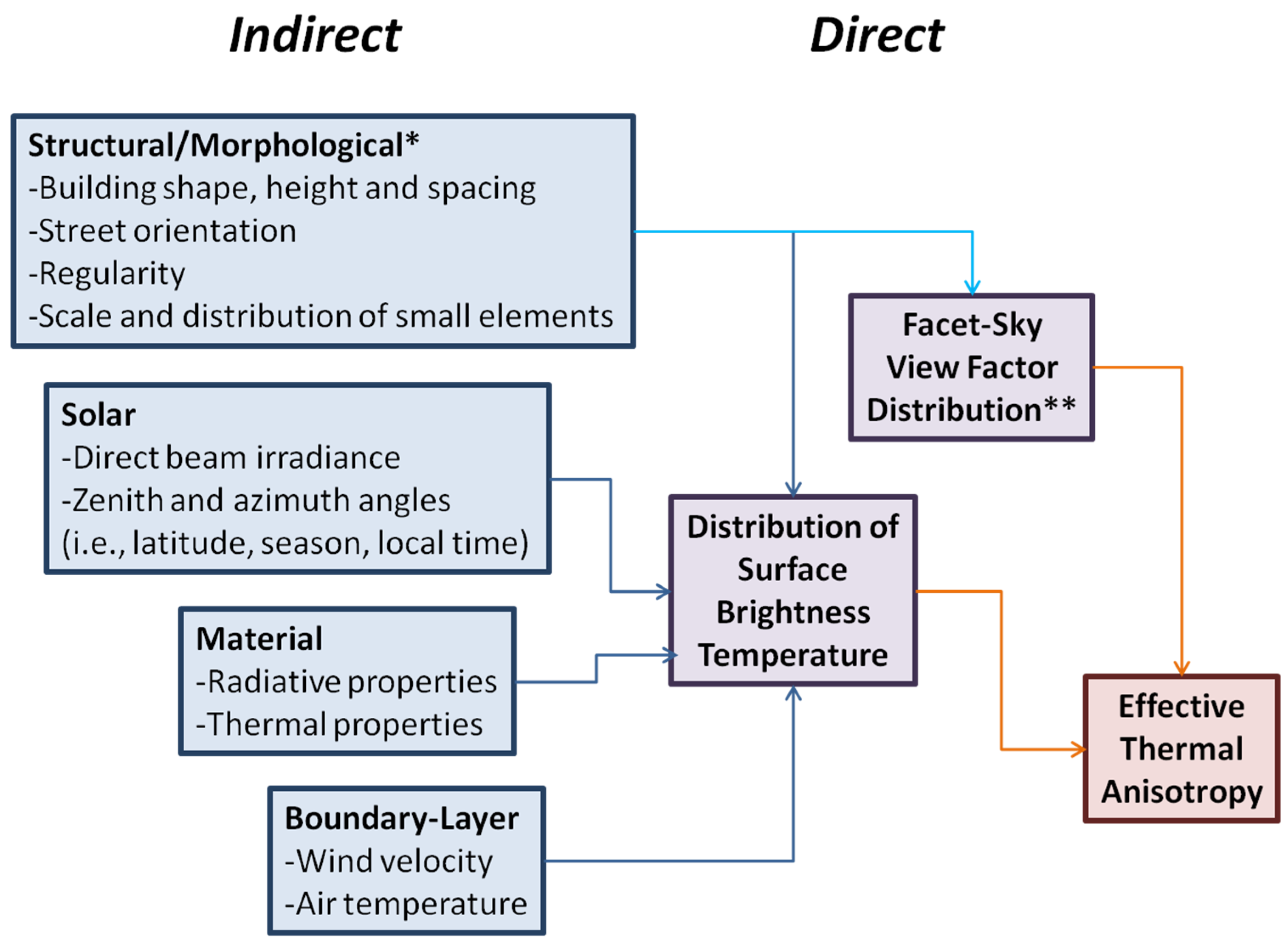
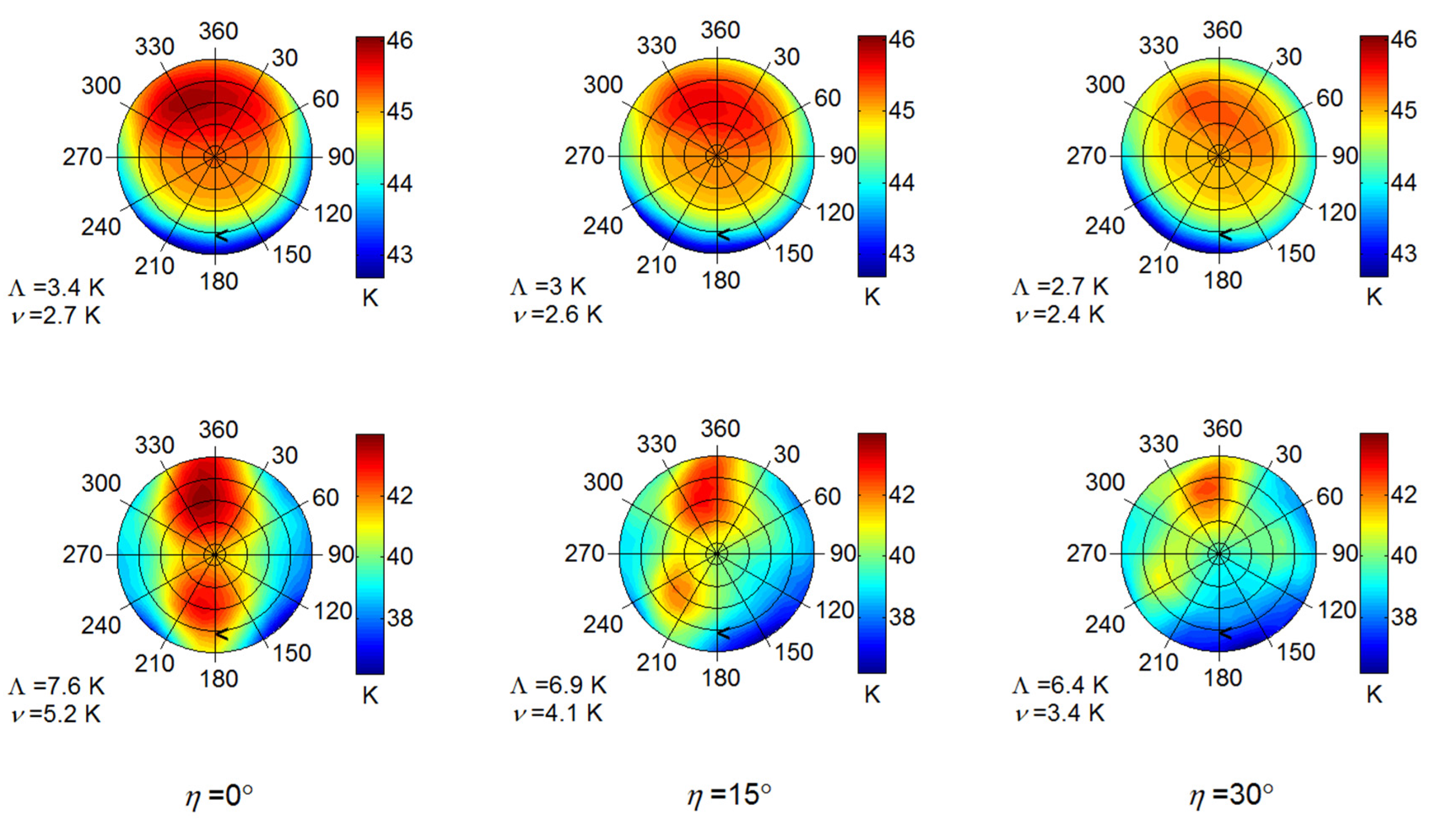
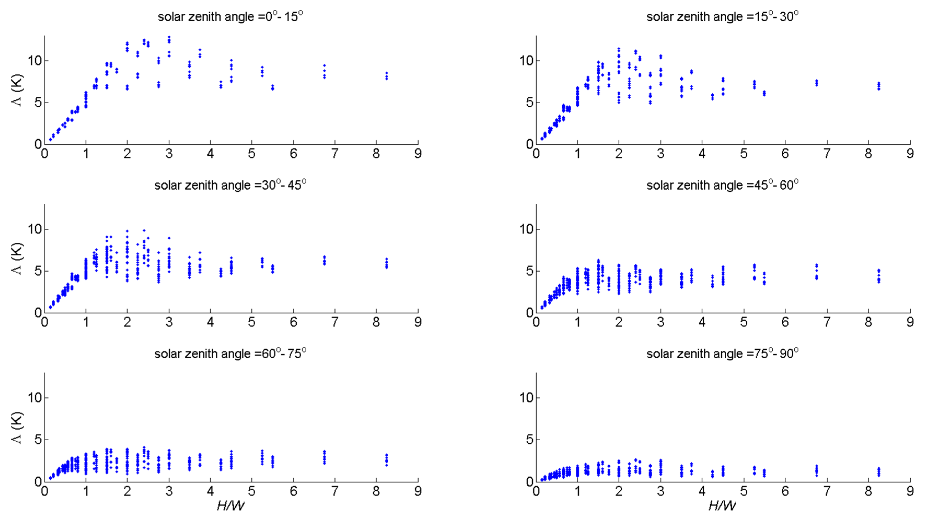
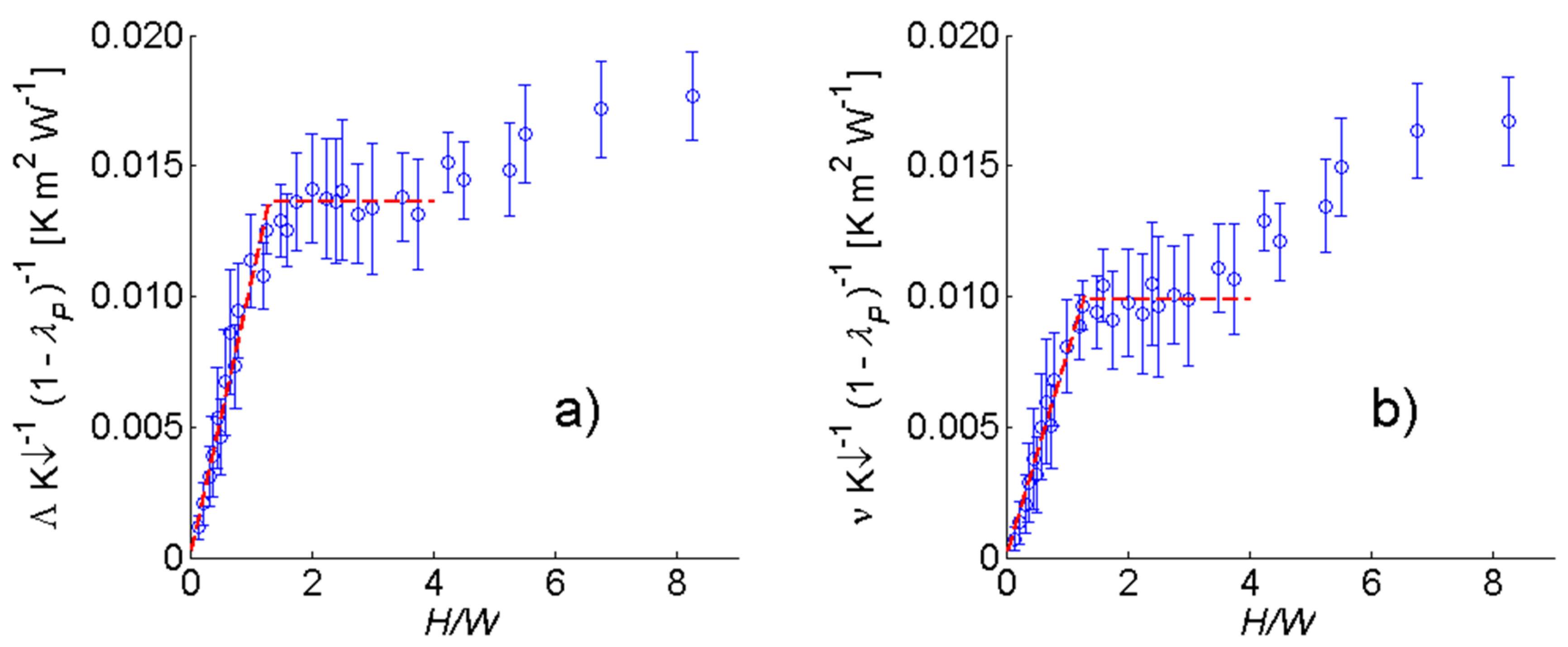
  • Urban effective anisotropy depends strongly on solar elevation and irradiance. It is increased for smaller solar zenith angle and greater irradiance. When normalized by solar irradiance (or roof surface temperature), anisotropy magnitude is independent of solar zenith angle.
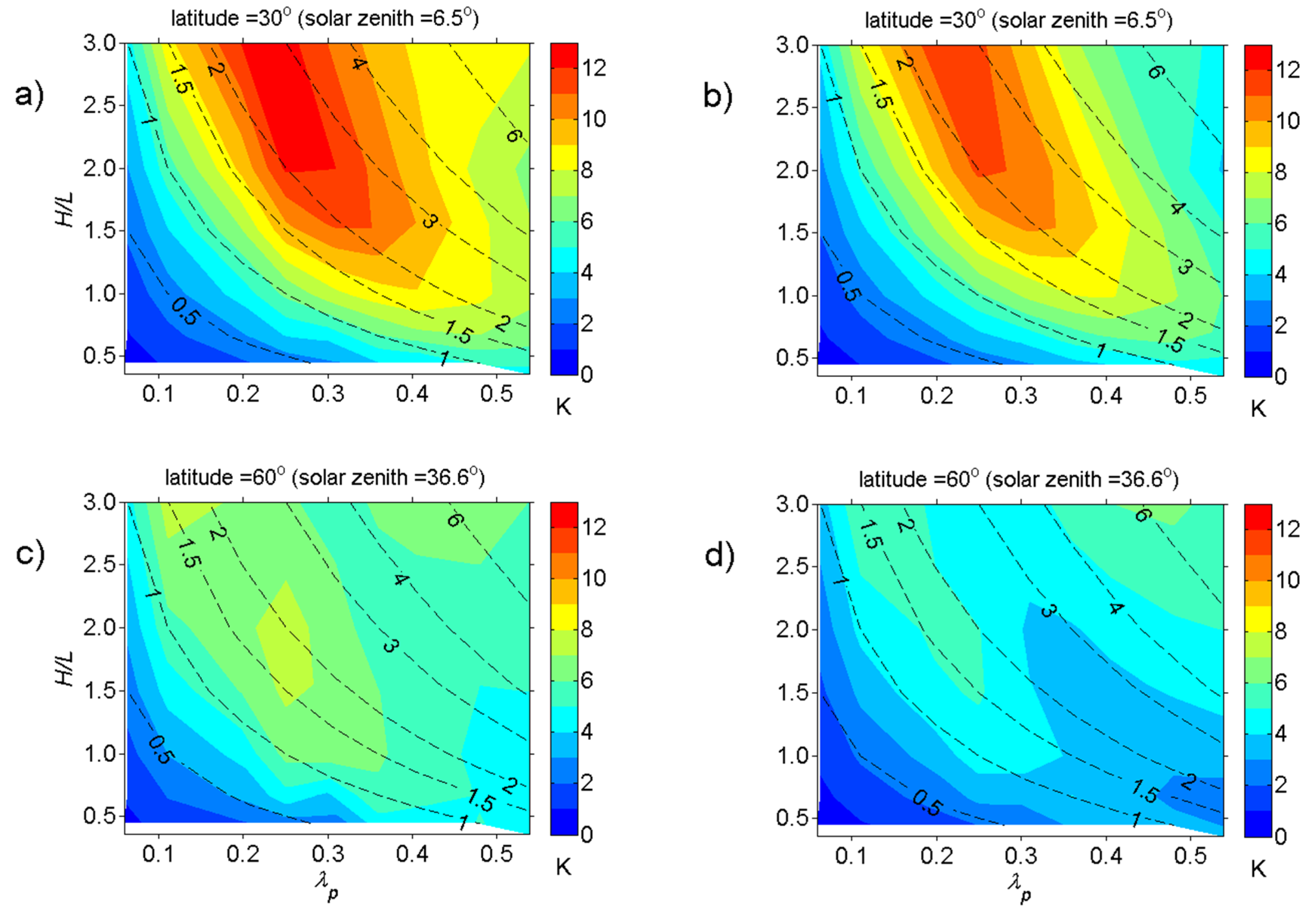
  • Urban effective anisotropy depends strongly on urban morphology, in particular, the ratio of building height to street width (H/W). It is maximized for H/W ≈ 1.5–3.0, and within this range it is greater for tall, moderately-spaced buildings than for shorter, closely-spaced buildings. Normalizing anisotropy magnitude by canyon (non-building) plan area (1 – λP) removes this dependence on building shape and spacing, strengthening the relation between anisotropy and H/W.
  • Modelled effective thermal anisotropy increases linearly as a function of H/W for H/W < 1.25 (approx.), with a slope that depends on maximum sensor off-nadir angle. For a maximum off-nadir angle of 45°, modeled anisotropy magnitude (in K) is Λ = 0.011 K↓ (1 – λP) H/W over this range of H/W, where K↓ is solar irradiance on a flat surface in W·m−2. This is considered a minimum estimate of anisotropy magnitude for real urban neighbourhoods because small scale structure, tree crowns and other neighbourhood features are neglected.
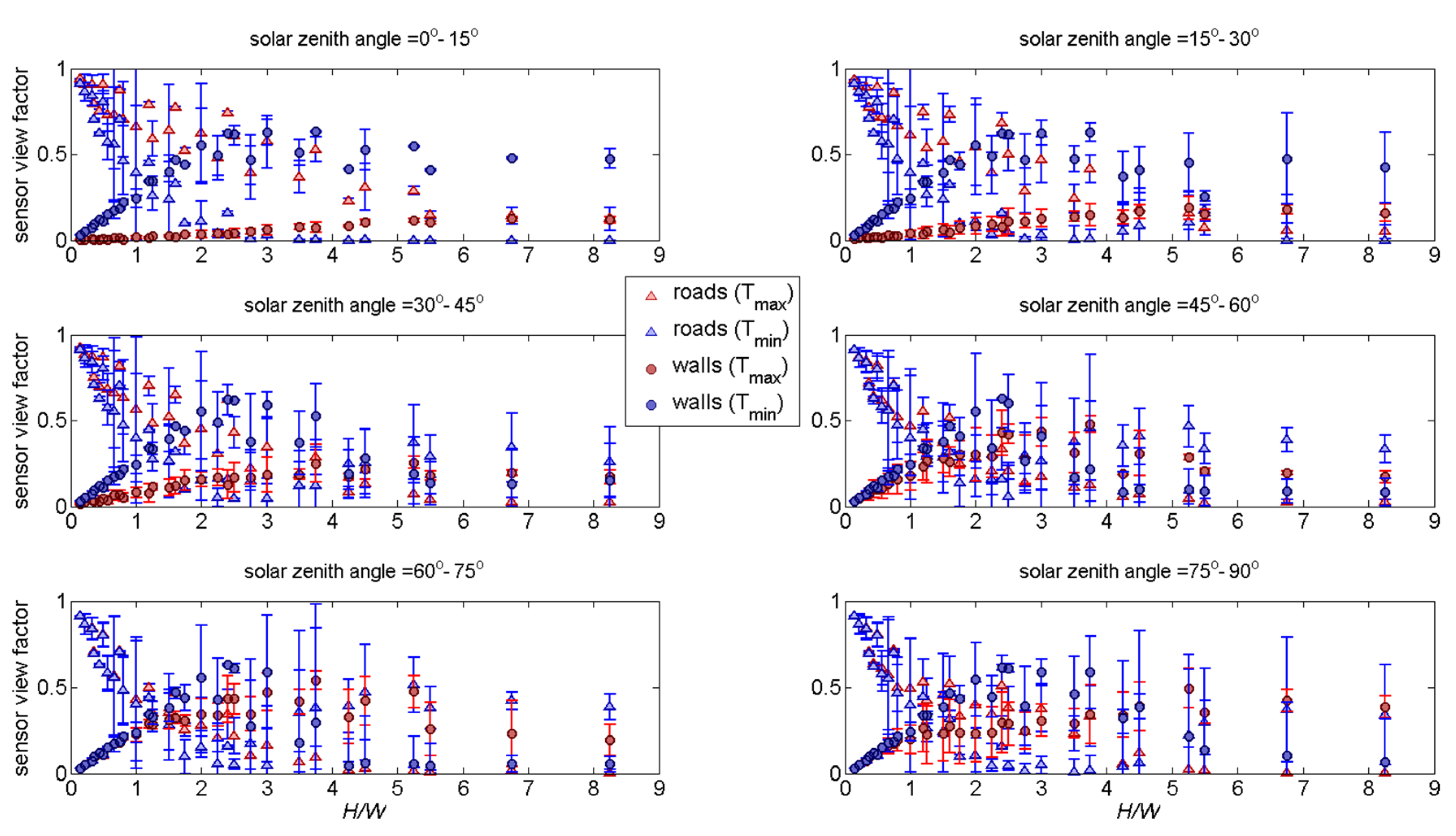
  • Variation of minimum brightness temperature with H/W controls the dependence of anisotropy on H/W more than the corresponding variation of maximum brightness temperature. Cool shaded walls are critical to production of anisotropy for H/W < 3.0.
TUF3D-SUM simulations of four “local climate zones” [41] at two latitudes provide some practical guidance:
  • Compact and high-rise zones generate greater anisotropy than an “open low-rise” (e.g., suburban) zone. With lower solar elevation angles (i.e., higher latitude), the difference is reduced: the “open low-rise” zone changes little, while the compact and highrise zones’ anisotropy is reduced.
  • Regularity of street orientation increases anisotropy. For this limited sample of solar angles and urban geometries, it represents 3%–31% of anisotropy magnitude depending on morphology and time of day (solar elevation).
  • Building shape and density, i.e., urban morphology, more strongly modulate anisotropy than material radiative and thermal properties.
In future work, relations between indirect factors, direct factors and effective anisotropy (Figure 1) should be more fully elucidated. Some particular focii should be: more realistic urban geometries, including variable building heights, trees [55,56] and ground-level vegetation, and small scale structures [37], which appear to be of particular importance (Section 3.3). Meteorological factors, in particular wind speed, were held constant in the present simulations, and are potentially important modulating factors of anisotropy [26]. Additionally, future work should more systematically investigate the variation of urban anisotropy with sensor off-nadir angle.
The present work is the first systematic investigation of daytime urban anisotropy magnitude and of its morphological causation. It confirms that neighbourhood geometry is a primary determinant of anisotropy magnitude, in particular the ratio between building height and building spacing, as well as solar factors, in particular shortwave radiation flux density.

Acknowledgments

Thanks are due to Daniel Dyce for helpful discussions. This work was funded by an NSERC Discovery Grant awarded to J.A.V.

Author Contributions

E.S.K. and J.A.V. conceived the experiments; E.S.K. designed and performed the model coupling, evaluation and sensitivity experiments; E.S.K wrote the paper with contributions from J.A.V.

Conflicts of Interest

The authors declare no conflict of interest.

Abbreviations

The following abbreviations are used in this manuscript:
FOV
Field of view
TUF3D
Temperature of Urban Facets in 3-D
SUM
Surface–sensor–sun Urban Model
AVHRR
Advanced Very High Resolution Radiometer
MODIS
Moderate-resolution Imaging Spectroradiometer
LST
Local solar time
LCZ
Local climate zone

References

  1. ReferencesOke, T.R. The urban energy balance. Prog. Phys. Geogr. 1988, 12, 471–508. [Google Scholar]
  2. Li, Z.-L.; Wu, H.; Wang, N.; Qiu, S.; Sobrino, J.A.; Wan, Z.; Tang, B.-H.; Yan, G. Land surface emissivity retrieval from satellite data. Int. J. Remote Sens. 2013, 34, 3084–3127. [Google Scholar] [CrossRef]
  3. Voogt, J.A.; Oke, T.R. Thermal remote sensing of urban climates. Remote Sens. Environ. 2003, 86, 370–384. [Google Scholar]
  4. Weng, Q. Thermal infrared remote sensing for urban climate and environmental studies: Methods, applications, and trends. ISPRS J. Photogram. Remote Sens. 2009, 64, 335–344. [Google Scholar] [CrossRef]
  5. Li, Z.-L.; Tang, B.-H.; Wu, H.; Ren, H.; Yan, G.; Wan, Z.; Trigo, I.F.; Sobrino, J.A. Satellite-derived land surface temperature: Current status and perspectives. Remote Sens. Environ. 2013, 131, 14–37. [Google Scholar] [CrossRef]
  6. Norman, J.M.; Divakarla, M.; Goel, N.S. Algorithms for extracting information from remote thermal-IR observations of the Earth’s surface. Remote Sens. Environ. 1995, 51, 157–168. [Google Scholar] [CrossRef]
  7. Voogt, J.A.; Oke, T.R. Effects of urban surface geometry on remotely-sensed surface temperature. Int. J. Remote Sens. 1998, 19, 895–920. [Google Scholar] [CrossRef]
  8. Oke, T.R. Boundary Layer Climates; Routledge: London, UK, 1987. [Google Scholar]
  9. Lagouarde, J.-P.; Kerr, Y.H.; Brunet, Y. An experimental study of angular effects on surface temperature for various plant canopies and bare soils. Agric. For. Meteorol. 1995, 77, 167–190. [Google Scholar] [CrossRef]
  10. Chehbouni, A.; Nouvellon, Y.; Kerr, Y.H.; Moran, M.S.; Watts, C.; Prevot, L.; Goodrich, D.C.; Rambal, S. Directional effect on radiative surface temperature measurements over a semiarid grassland site. Remote Sens. Environ. 2001, 76, 360–372. [Google Scholar] [CrossRef]
  11. Menenti, M.; Jia, L.; Li, Z.-L.; Djepa, V.; Wang, J.; Stoll, M.P.; Su, Z.; Rast, M. Estimation of soil and vegetation temperatures with multiangular thermal infrared observations. IMGRASS, HEIFE and SGP 1997 experiments. J. Geophys. Res. 2001, 106, 11997–12010. [Google Scholar] [CrossRef]
  12. Rasmussen, M.O.; Göttsche, F.; Olesen, F.; Sandholt, I. Directional effects on land surface temperature estimation from Meteosat Second Generation for savanna landscapes. IEEE Trans. Geosci. Remote Sens. 2011, 49, 4458–4468. [Google Scholar] [CrossRef]
  13. McGuire, M.J.; Balick, L.K.; Smith, J.A.; Hutchison, B.A. Modeling directional thermal radiance from a forest canopy. Remote Sens. Environ. 1989, 29, 169–186. [Google Scholar] [CrossRef]
  14. Lagouarde, J.-P.; Ballans, H.; Moreau, P.; Guyon, D.; Coraboeuf, D. Experimental study of brightness surface temperature angular variations of Maritime Pine (Pinus pinaster) stands. Remote Sens. Environ. 2000, 72, 17–34. [Google Scholar] [CrossRef]
  15. Ermida, S.L.; Trigo, I.F.; Dacamara, C.C.; Göttsche, F.M.; Olesen, F.S.; Hulley, G. Validation of remotely sensed surface temperature over an oak woodland landscape—The problem of viewing and illumination geometries. Remote Sens. Environ. 2014, 148, 16–27. [Google Scholar] [CrossRef]
  16. Lipton, A.E.; Ward, J.M. Satellite-view biases in retrieved surface temperatures in mountain areas. Remote Sens. Environ. 1997, 60, 92–100. [Google Scholar] [CrossRef]
  17. Minnis, P.; Khaiyer, M.M. Anisotropy of land surface skin temperature derived from satellite data. J. Appl. Meteorol. 2000, 39, 1117–1129. [Google Scholar] [CrossRef]
  18. Pinheiro, A.C.T.; Privette, J.L.; Mahoney, R.; Tucker, C.J. Directional effects in a daily AVHRR land surface temperature dataset over Africa. IEEE Trans. Geosci. Remote Sens. 2004, 42, 1941–1954. [Google Scholar] [CrossRef]
  19. Trigo, I.F.; Peres, L.F.; DaCamara, C.C.; Freitas, S.C. Thermal land surface emissivity retrieved from SEVIRI/Meteosat. IEEE Trans. Geosci. Remote Sens. 2008, 46, 307–315. [Google Scholar] [CrossRef]
  20. Rao, P.K. Remote sensing of urban heat islands from environmental satellite. Bull. Am. Meteorol. Soc. 1972, 53, 647–648. [Google Scholar]
  21. Roth, M.; Oke, T.R.; Emery, W.J. Satellite-derived urban heat island from three coastal cities and the utilization of such data in urban climatology. Int. J. Rem. Sens. 1989, 10, 1699–1720. [Google Scholar] [CrossRef]
  22. Iino, A.; Hoyano, A. Development of a method to predict the heat island potential using remote sensing and GIS data. Energy. Build. 1996, 23, 199–205. [Google Scholar] [CrossRef]
  23. Lagouarde, J.-P.; Moreau, P.; Irvine, M.; Bonnefond, J.M.; Voogt, J.A.; Solliec, F. Airborne experimental measurements of the angular variations in surface temperature over urban areas: Case study of Marseille (France). Remote Sens. Environ. 2004, 93, 443–462. [Google Scholar] [CrossRef]
  24. Sugawara, H.; Takamura, T. Longwave radiation flux from an urban canopy: Evaluation via measurements of directional radiometric temperature. Remote Sens. Environ. 2006, 104, 226–237. [Google Scholar] [CrossRef]
  25. Lagouarde, J.P.; Irvine, M. Directional anisotropy in thermal infrared measurements over Toulouse city centre during the CAPITOUL measurement campaigns: First results. Meteorol. Atmos. Phys. 2008, 102, 173–185. [Google Scholar] [CrossRef]
  26. Lagouarde, J.P.; Hénon, A.; Kurz, B.; Moreau, P.; Irvine, M.; Voogt, J.; Mestayer, P. Modelling daytime thermal infrared directional anisotropy over Toulouse city centre. Remote Sens. Environ. 2010, 114, 87–105. [Google Scholar] [CrossRef]
  27. Lagouarde, J.P.; Hénon, A.; Irvine, M.; Voogt, J.; Pigeon, G.; Moreau, P.; Masson, V.; Mestayer, P. Experimental characterization and modelling of the nighttime directional anisotropy of thermal infrared measurements over an urban area: Case study of Toulouse (France). Remote Sens. Environ. 2012, 117, 19–33. [Google Scholar] [CrossRef]
  28. Voogt, J.A.; Soux, C.A. Methods for the assessment of representative urban surface temperatures. In Proceedings of the 3rd Symposium on the Urban Environment (AMS), Davis, CA, USA, 14–18 August 2000; pp. 179–180.
  29. Adderley, C.; Christen, A.; Voogt, J.A. The effect of radiometer placement and view on inferred directional and hemispheric radiometric temperatures of a urban canopy. Atmos. Meas. Tech. 2015, 8, 1891–1933. [Google Scholar] [CrossRef]
  30. Nichol, J.E. Visualisation of urban surface temperatures derived from satellite images. Int. J. Remote Sens. 1998, 19, 1639–1649. [Google Scholar] [CrossRef]
  31. Voogt, J.A.; Oke, T.R. Complete urban surface temperatures. J. Appl. Meteorol. 1997, 36, 1117–1132. [Google Scholar] [CrossRef]
  32. Voogt, J.A.; Grimmond, C.S.B. Modeling surface sensible heat flux using surface radiative temperatures in a simple urban area. J. Appl. Meteorol. 2000, 39, 1679–1699. [Google Scholar] [CrossRef]
  33. Chappell, A.; van Pelt, S.; Zobeck, T.; Dong, Z. Estimating aerodynamic resistance of rough surfaces using angular reflectance. Remote Sens. Environ. 2010, 114, 1462–1470. [Google Scholar] [CrossRef]
  34. Krayenhoff, E.S.; Voogt, J.A. A microscale three-dimensional urban energy balance model for studying surface temperatures. Bound.-Layer Meteorol. 2007, 123, 433–461. [Google Scholar] [CrossRef]
  35. Soux, A.; Voogt, J.A.; Oke, T.R. A model to calculate what a remote sensor sees of an urban surface. Bound.-Layer Meteorol. 2004, 112, 109–132. [Google Scholar] [CrossRef]
  36. Krayenhoff, E.S. A Microscale 3-D Urban Energy Balance Model for Studying Surface Temperatures. Master’s Thesis, Department of Geography, Western University, London, ON, Canada, 2005. [Google Scholar]
  37. Voogt, J.A. Assessment of an urban sensor view model for thermal anisotropy. Remote Sens. Environ. 2008, 112, 482–495. [Google Scholar] [CrossRef]
  38. Voogt, J.A.; Krayenhoff, E.S. Modeling urban thermal anisotropy. In Proceedings of the 5th International Symposium Remote Sensing of Urban Areas, Phoenix, AZ, USA, 14–16 March 2005.
  39. Krayenhoff, E.S.; Voogt, J.A. Combining sub-facet scale urban energy balance and sensor-view models to investigate effective thermal anisotropy on city structure. In Proceedings of the 7th Symposium on the Urban Environment, American Meteorological Society, San Diego, CA, USA, 10–13 September 2007.
  40. Henon, A.; Mestayer, P.G.; Lagouarde, J.-P.; Voogt, J.A. An urban neighborhood temperature and energy study from the CAPITOUL experiment with the SOLENE model. Theor. Appl. Climatol. 2012, 110, 197–208. [Google Scholar] [CrossRef]
  41. Stewart, I.D.; Oke, T.R. Local climate zones for urban temperature studies. Bull. Am. Meteorol. Soc. 2012, 93, 1879–1900. [Google Scholar] [CrossRef]
  42. Ashdown, I. Radiosity: A Programmers Perspective; John Wiley & Sons: New York, NY, USA, 1994. [Google Scholar]
  43. Mills, G.M. An urban canopy-layer climate model. Theor. Appl. Climatol. 1997, 57, 229–244. [Google Scholar] [CrossRef]
  44. Masson, V.; Grimmond, C.S.B.; Oke, T.R. Evaluation of the town energy balance (TEB) scheme with direct measurements from dry districts in two cities. J. Appl. Meteorol. 2002, 41, 1011–1026. [Google Scholar]
  45. Kurz, B. Modelisation De L’anisotropie Directionelle de la Temperature de Surface: Application au Cas de Milieu Forestiers et Urbains. Ph.D. Thesis, University of Toulouse, Toulouse, France, 2009. [Google Scholar]
  46. Rotach, M.W.; Vogt, R.; Bernhofer, C.; Batchvarova, E.; Christen, A.; Clappier, A.; Feddersen, B.; Gryning, S.-E.; Martucci, G.; Mayer, H.; et al. BUBBLE—An urban boundary layer meteorology project. Theor. Appl. Climatol. 2005, 81, 231–261. [Google Scholar] [CrossRef]
  47. Iqbal, M. An Introduction to Solar Radiation; Academic Press: Toronto, ON, Canada, 1983. [Google Scholar]
  48. Prata, A.J. A new long-wave formula for estimating downward clear-sky radiation at the surface. Q. J. R. Meteorol. Soc. 1996, 122, 1127–1151. [Google Scholar] [CrossRef]
  49. Stull, R.B. Meteorology for Scientists and Engineers, 2nd ed.; Brooks/Cole: Pacific Grove, CA, USA, 2000; p. 502. [Google Scholar]
  50. Oke, T.R. Street design and urban canopy layer climate. Energy Build. 1988, 11, 103–113. [Google Scholar] [CrossRef]
  51. Huang, H.; Liu, Q.; Qin, W.; Du, Y.; Li, X. Temporal patterns of thermal emission directionality of crop canopies. J. Geophys. Res. 2011, 116, D06114. [Google Scholar] [CrossRef]
  52. Stewart, I.D.; Oke, T.R.; Krayenhoff, E.S. Evaluation of the local climate zone scheme using temperature observations and model simulations. Int. J. Climatol. 2014, 34, 1062–1080. [Google Scholar] [CrossRef]
  53. Krayenhoff, E.S.; Voogt, J.A. Impacts of urban albedo increase on local air temperature at daily-annual time scales: Model results and synthesis of previous work. J. Appl. Meteorol. Climatol. 2010, 49, 1634–1648. [Google Scholar] [CrossRef]
  54. Kimes, D.S. Remote sensing of row crop structure and component temperatures using directional radiometric temperatures and inversion techniques. Remote Sens. Environ. 1983, 13, 33–55. [Google Scholar] [CrossRef]
  55. Dyce, D.R. A Sensor View Model to Investigate the Influence of Tree Crowns on Effective Urban Thermal Anisotropy. Master’s Thesis, Department of Geography, Western University, London, ON, Canada, 2014. [Google Scholar]
  56. Dyce, D.R.; Voogt, J.A. The influence of tree crowns on effective urban thermal anisotropy. In Proceedings of the ICUC9—9th International Conference on Urban Climate/12th Symposium on the Urban Environment, Toulouse, France, 20–24 July 2015.

