Article

Vertical Profiling of Volcanic Ash from the 2011 Puyehue Cordón Caulle Eruption Using IASI

1
Belgian Institute for Space Aeronomy, 3 Avenue Circulaire, Brussels 1180, Belgium
2
Department of Analytical Chemistry, Ghent University, Krijgslaan 281 S12, Ghent 9000, Belgium
3
German Aerospace Center (DLR), German Remote Sensing Datacenter (DFD), Oberpfaffenhofen, 82334 Wessling, Germany
*
Authors to whom correspondence should be addressed.
These authors contributed equally to this work.
Remote Sens. 2016, 8(2), 103; https://doi.org/10.3390/rs8020103
Submission received: 18 September 2015 / Revised: 8 January 2016 / Accepted: 20 January 2016 / Published: 29 January 2016
(This article belongs to the Special Issue Aerosol and Cloud Remote Sensing)

Abstract

:
Volcanic ash is emitted by most eruptions, sometimes reaching the stratosphere. In addition to its climate effect, ash may have a significant impact on civilian flights. Currently, the horizontal distribution of ash aerosols is quite extensively studied, but not its vertical profile, while of high importance for both applications mentioned. Here, we study the sensitivity of the thermal infrared spectral range to the altitude distribution of volcanic ash, based on similar work that was undertaken on mineral dust. We use measurements by the Infrared Atmospheric Sounding Interferometer (IASI) instruments onboard the MetOp satellite series. The retrieval method that we develop for the ash vertical profile is based on the optimal estimation formalism. This method is applied to study the eruption of the Chilean volcano Puyehue, which started on the 4th of June 2011. The retrieved profiles agree reasonably well with Cloud-Aerosol LiDAR with Orthogonal Polarization (CALIOP) measurements, and our results generally agree with literature studies of the same eruption. The retrieval strategy presented here therefore is very promising for improving our knowledge of the vertical distribution of volcanic ash and obtaining a global 3D ash distribution twice a day. Future improvements of our retrieval strategy are also discussed.

Graphical Abstract

1. Introduction

Volcanoes are ubiquitous on our planet. On average, there are 50 to 70 eruptions per year. Many emit ash particles into the atmosphere where they may cause damage to aircraft (reduce visibility, clog sensors, at worst block the engines; see, for example, [1,2,3,4]). During the time aerosols spend in the atmosphere (from days to months depending on the eruption intensity, the emission altitude, etc.) [5], they also impact the radiative balance of our planet. Indeed, these particles scatter and absorb the incoming and reflected solar light: this is the short-wave (SW) direct effect. Because almost all ash particles are coarse particles [6], they also scatter and absorb the longer wavelengths from the thermal infrared emission from the surface and the atmosphere: this is the long-wave (LW) direct effect. Following Planck and Kirchoff’s laws, ash particles also emit infrared radiation themselves. In addition to these direct effects, aerosols show several indirect effects due to their interaction with clouds [7,8]. For example, they can act as cloud or ice condensation nuclei to modify the lifetime or albedo of a cloud. Additionally being inside a cloud increases the atmospheric lifetime of aerosols. All of these radiative effects of ash aerosols depend on their vertical distribution. Indeed, the thermal emission of the mineral aerosols depends intrinsically on their temperature, therefore on their altitude. The indirect effects through the interaction of ash and clouds also depend on their relative vertical location [5].
The global impact of aerosols on the radiation budget of the Earth is called the aerosol radiative forcing (RF). The RF is the net change in energy at a certain altitude due to a changed parameter in the climate system. According to the Fifth Assessment Report (AR5) of the Intergovernmental Panel on Climate Change in 2013 (IPCC [9]), aerosols in general have a slightly negative RF. However, a large uncertainty exists on this RF, including the possibility that it is actually positive (i.e., positive values are within the error bar). Regarding volcanic ash (and mineral dust), a non-negligible part of the RF uncertainties comes from the very poor knowledge about the vertical distribution of the aerosol.
Because of their hazardous effects, ash aerosols have been extensively studied. In Europe alone, the recurrent eruptions of Etna and the recent eruption of Eyjafjallajökull resulted in much scientific research. Using remote sensing techniques, different properties of ash clouds are retrieved, mainly the geographical dispersion, the particle size and optical depth (e.g., [10,11,12,13,14,15,16]). SO 2 is sometimes used as a proxy for ash clouds (e.g., [17,18]). Many efforts have also been made to design new ways of retrieving volcanic plume heights (e.g., [19,20,21,22,23,24,25]), also sometimes based on SO 2 . These methods retrieve the volcanic plume height, but they only retrieve single-layer altitudes, either top altitude or an average. This obviously is sufficient as long as there is only one ash layer in the atmosphere. However, there is sometimes more than one layer of ash in the atmosphere, for example when different events within the same eruption inject ash at different altitudes.
There is, to the authors’ knowledge, currently no availability of ash aerosol vertical profiles with sufficient time and space coverage to allow climate applications. The only satellite instrument that provides vertical profiles of ash (together with other aerosols) is the Cloud-Aerosol LiDAR with Orthogonal Polarization (CALIOP) [26]. CALIOP has the advantage of an extremely high vertical and horizontal resolution, but the drawback of a very poor geographic coverage (15 orbits with a 70-m swath width each day around the globe). If one were able to retrieve vertical information on ash aerosols from thermal infrared (TIR) measurements by instruments like IASI onboard the MetOp satellite series [27], it would be possible to obtain global coverage twice a day, with a time coverage spanning 2006 to 2025 at least. This dataset would greatly benefit both climate studies and the aviation business.
Ash particles are not the only aerosols that impact the TIR radiation. The presence of other aerosol types together with ash may influence ash retrievals. Clarisse et al. [28] studied differences in extinction in the TIR “atmospheric window” due to different aerosol types. The “atmospheric window” is the spectral region between about 750 and 1250 cm - 1 , so called because of its particularly high transmittance in clear sky situations, allowing the retrieval of the surface temperature. The authors compared five types of aerosols: sand, volcanic ash, sulfuric acid, biomass burning and ice. For sand and ash, a clear V shape is observed between 800 and 1200 cm - 1 . The signatures of sand and ash are quite alike, due to the fact that they are both minerals. This makes it quite difficult to distinguish between them, but not impossible, as was demonstrated by Clarisse et al. [29]. For ice particles, strong extinction is observed in the atmospheric window. The ice particles extinguish the radiation most significantly around 800 cm - 1 , and less for increasing wavenumbers up to the ozone absorption band at 1050 cm - 1 , forming an ascending slope in the spectrum where minerals cause a descending slope. From 1100 to 1200 cm - 1 , ice particles cause a flat reduction of radiation. Because of this spectral signature of ice particles, which is somewhat opposite that of dust and ash, the mineral aerosol retrievals will be more difficult in the presence of ice, maybe even impossible if there is a large amount of ice particles (however, we are not yet able to quantify this). In particular, this affects the ash retrievals, as ice is often found mixed with ash. Sulfuric acid and biomass burning both cause only a weak extinction, making it difficult to retrieve their properties from TIR measurements. On the other hand, their presence in the sampled atmospheric air mass is then not an issue for ash retrievals from TIR radiances.
This work presents the first retrievals of volcanic ash vertical profiles (with up to two degrees of freedom) from TIR measurements by the nadir-viewing Infrared Atmospheric Sounding Interferometer (IASI). As such, the development of the method itself is an important part of this paper. First, we use a radiative transfer forward model to study the sensitivity of the IASI radiances to the presence and altitude of ash aerosols, in the full IASI spectral range. The spectral windows experiencing the largest sensitivity to ash aerosols are investigated further by the computation of derivatives of the radiance with respect to the aerosol concentrations at different altitudes (radiance Jacobians). The impact of differences in the aerosol parameters is also briefly studied. Based on these findings, a retrieval strategy for ash vertical profiles is designed using Rodgers’ optimal estimation (OE) formalism [30]. This strategy is called mineral aerosol profiling from infrared radiances (MAPIR). The retrieval strategy is then applied to the Plinian eruption from a fissure in the Puyehue-Cordón Caulle Volcanic Complex in central Chile, which began on the 4th of June 2011 at 19:15 UTC. This eruption has already been studied from IASI measurements by Klüser et al. [31] using another method based on principal components analysis to retrieve the aerosol optical depth (AOD) and by Bignami et al. [13] using different sensors. In this work, we compare our results with both of these studies, in terms of ash detection, optical depth and altitude information. We also compare our retrieved vertical profiles with coinciding measurements by CALIOP on 16 June 2011 (no CALIOP data are available between the start of the eruption and that date).
The conclusion of this paper is that it is possible to retrieve reasonable vertical information about ash plumes from IASI measurements, with the ability to separate two ash layers, at least for the case studied here. This is a very promising result, considering the time and space coverage by IASI instruments, and the long-term availability of IASI data. To be able to generalize this work to any volcanic eruption, more work is required, as the sensitivity depends on the surface and atmospheric conditions and also because the ash particles vary in size and composition for each eruption.

2. Experimental Section

2.1. Satellite Data Characteristics

2.1.1. IASI

IASI is a nadir-viewing Fourier transform Michelson interferometer measuring the upwelling radiation in the thermal infrared window between 645 and 2760 cm - 1 (15.5 to 5 μm) with a spectral sampling of 0.25 cm - 1 and a resolution of 0.5 cm - 1 after apodization (Level 1c data). The instrument is developed by the Centre National d’Etudes Spatiales (CNES) in cooperation with the European Organisation for the Exploitation of Meteorological Satellites (EUMETSAT). It has an average radiometric noise around 9×10 - 7 W · cm - 2 (sr·cm - 1 ) - 1 or 0.2 K for a temperature of 280 K [27]. IASI has a swath width of 2130 km and an instantaneous field of view of four circles of 12 km in diameter at nadir. IASI flies on board the MetOp satellites on a mid-morning Sun-synchronous polar orbit (around 9:30 local solar Equator crossing time), allowing global coverage twice a day. The first satellite, MetOp-A, was launched in October 2006, and the second one, MetOp-B, was launched in September 2012. In 2018, the launch of a third satellite is planned, providing measurements up to probably 2025. An improved version of the IASI instrument is already planned to fly onboard the second generation of MetOp instruments, starting around 2021, for about 20 years of operations.

2.1.2. CALIOP

The Cloud-Aerosol LiDAR with Orthogonal Polarization (CALIOP) instrument is part of the Cloud-Aerosol LiDAR and Infrared Pathfinder Satellite Observations (CALIPSO) satellite. CALIPSO has a mid-afternoon Sun-synchronous polar orbit (13:30 Equator crossing local solar time). CALIOP is a LiDAR measuring actively at nadir. It has 2 lasers (532 and 1064 nm) that emit to the Earth with a diameter of 70 m at the surface, directly underneath the satellite. CALIOP measures the backscattered radiation at those wavelengths, which provides information about the scattering and extinction properties of clouds and aerosols as a function of their altitude. CALIOP measures day and night every 330 m along its track, with a vertical resolution of 30 m. It covers the Earth in 16 days [26].

2.2. Development of the Retrieval Algorithm and Strategy for Ash Vertical Profiles

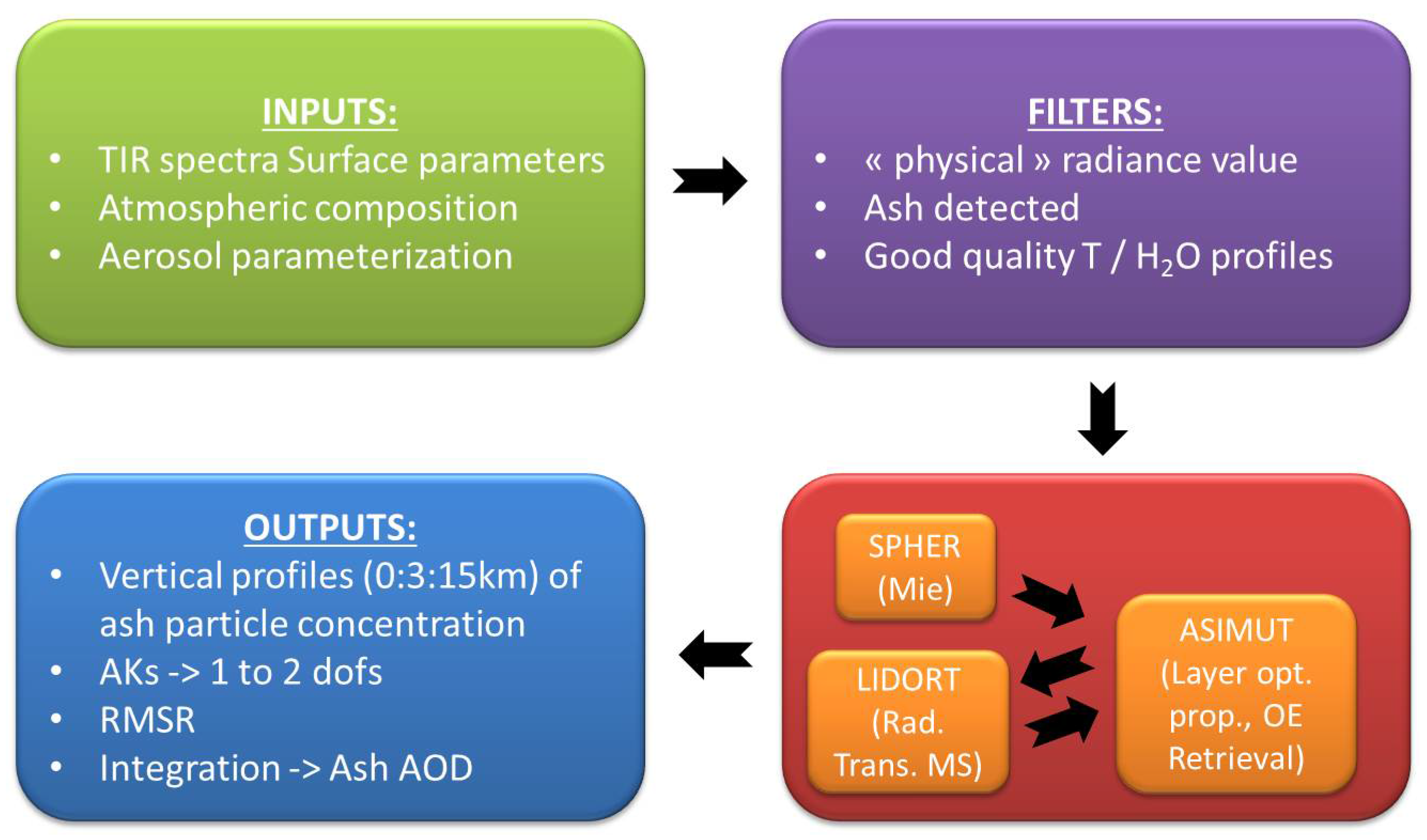
2.2.1. The MAPIR Algorithm and Software

The retrieval of vertical profiles of volcanic ash presented here is based on the work by Vandenbussche et al. [32], who presented the first retrievals of vertical profiles of mineral dust from IASI measurements. However, as volcanic ash may be found at higher altitudes (dust is found mostly below 6 km), the establishment of the ash retrieval strategy requires further study of the altitude effects of the volcanic ash aerosols on the TIR radiance. The effect of refractive index and particle size may also be different and is therefore briefly studied. The retrieval scheme has been called mineral aerosol profiling from infrared radiances (MAPIR).
MAPIR is built on the ASIMUT software package [33] combined with the advanced radiative transfer code LInearized Discrete Ordinate Radiative Transfer (LIDORT) [34] and the Mie code from M. Mishchenko [35]. ASIMUT performs the retrieval using Rodgers OE formalism [30]. It computes surface and atmospheric emissions at each wavelength (using the Planck formula), total optical depth (OD), single scattering albedo (SSA) and scattering phase functions of each atmospheric layer, as well as the individual contributions (to OD, SSA and phase functions) of parameters for which Jacobians are requested. Gas extinction at each wavelength is computed line-by-line. ASIMUT then provides all of these surface and atmospheric parameters in the format needed by LIDORT. The Mie code calculates the aerosol single scattering albedo (SSA), extinction coefficients and scattering functions from a particle size distribution (PSD) and refractive index. LIDORT calculates the radiative transfer, including multiple scattering, and the necessary weighting functions (Jacobians), being in our case the derivatives of the radiance with respect to the concentration of the aerosols at different altitudes.

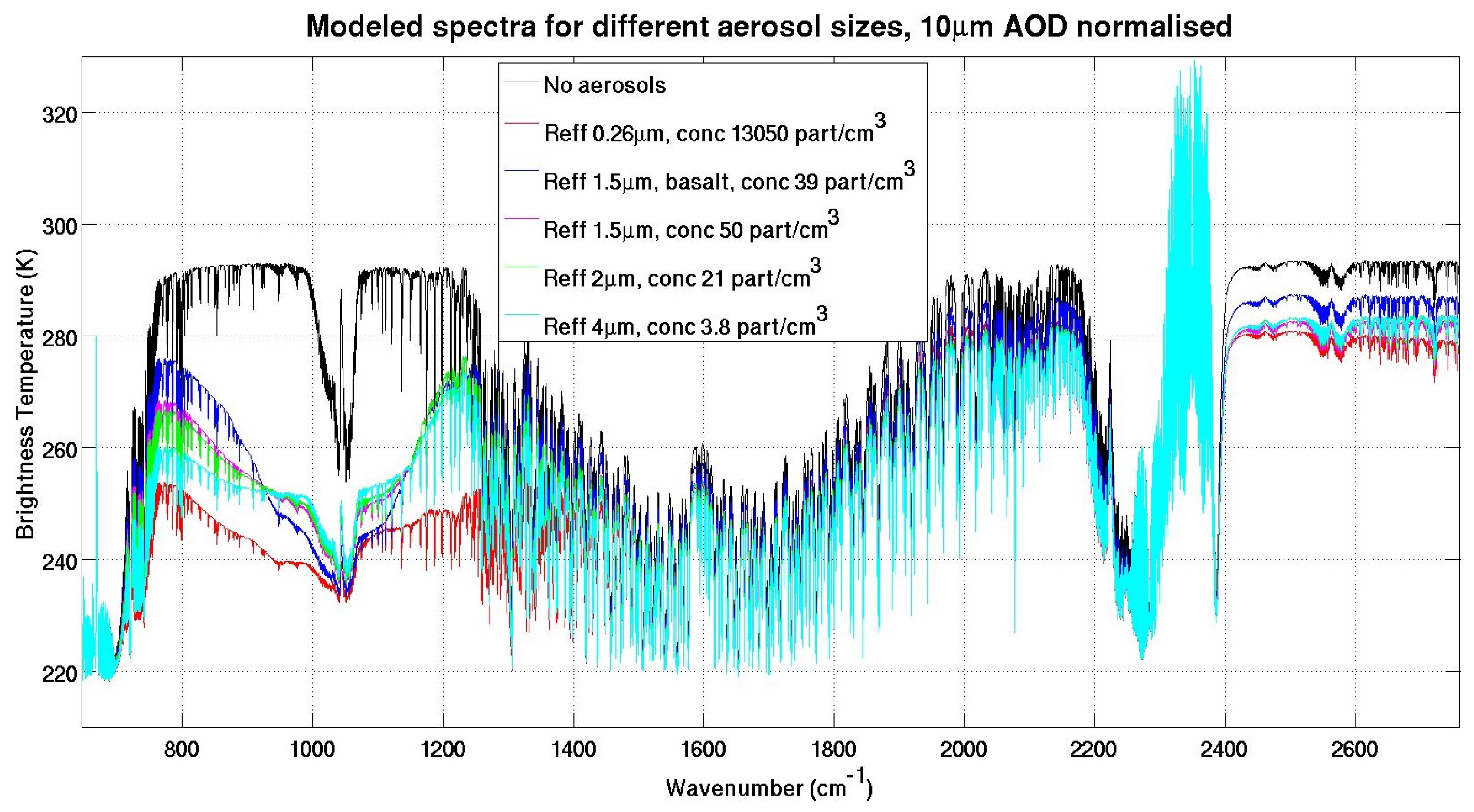
2.2.2. Aerosol Model Selection

The first step of this analysis is to select appropriate data to model the ash aerosols. Considering the software, a particle size distribution and a refractive index have to be ingested in the Mie computation. We have chosen the “volcanic ash” refractive index from the gestion et étude des informations spectroscopiques atmosphriques (GEISA)/high-resolution transmission molecular absorption (HITRAN) database [36,37], which is based on measurements by Volz [38,39] and Shettle and Fenn [40] on feldspar and perlite ash. We also tested the refractive index of basalt given by Pollack et al. [41]. We assume a lognormal particle size distribution (PSD) as described for example in Clarisse et al. [28]:
N r = N 0 2 π l n σ g r e x p ( - l n 2 ( r r g ) 2 l n 2 σ g )
with N 0 being the total amount of aerosols, r g the geometrical average radius and σ g the average standard deviation. The effective radius r e often given in the literature is linked to the previous parameters as follows:
r e = r g e x p ( 2 . 5 l n 2 σ g )
We modeled spectra with four different aerosol sizes to evaluate their impact on the IASI spectral range: small ( r g = 0 . 2 μ m and σ = 1 . 4 , r e = 0 . 26 μ m), medium ( r g = 0 . 45 μ m and σ = 2 , r e = 1 . 5 μ m), large ( r g = 0 . 6 μ m and σ = 2 , r e = 2 μ m) and extra large particles ( r g = 1 . 2 μ m and σ = 2 , r e = 4 μ m). The particles are assumed to be spherical, as is often the case in TIR mineral aerosol retrievals; see, for example, [12,28,32,42,43]. Indeed, while there might be non-spherical effects in the TIR, they are expected to be much less important than in the solar spectral window. In MAPIR, we consider these effects as being smaller than the effect of other aerosol parameter uncertainties.
We performed forward model simulations over the whole spectral range of IASI measurements, with one huge aerosol layer from 0 to 18 km for different aerosol sizes, using the refractive index from the GEISA/HITRAN database. An additional simulation has been done using the basalt refractive index of Pollack et al. [41], for the medium aerosol size. In each case, the aerosol concentration has been set so that the 10 μ m AOD amounts to the fixed value of 2.2; the latter value has been chosen because it makes the aerosol effects and their sensitivity to different aerosol physical parametrization easily observed. The atmospheric conditions for those simulations were typical of the conditions during the Puyehue eruption used as a test case in this work. Figure 1 shows the simulated spectra, and the legend contains the aerosol number concentration necessary to reach the desired optical depth. One important preliminary remark is that even though the AOD were normalized at 10 μ m, the different spectra do not match at that wavelength, because different particle properties also mean a different ratio between emission and extinction, the emission not being accounted for when computing the AOD. This is particularly visible as a difference between the almost non-scattering small particles (single scattering albedo close to zero) and the medium or large particles (single scattering albedo of about 0.55).
Figure 1. Modeled spectra without aerosols and for different aerosol sizes. Aerosols were placed from a 0- to 18-km altitude with a 10 μm (1000 cm - 1 ) aerosol optical depth (AOD) of 2.2. The dark blue spectrum has been modeled using the refractive index of basalt, while all of the others were obtained with the GEISA/HITRAN volcanic ash refractive index.
Remotesensing 08 00103 g001
For the small particles, the necessary aerosol number concentration to reach the desired AOD was extremely high (about 250-times that for the medium particles). Such a high concentration of small particles is improbable, meaning that the small particles’ effect is almost certainly negligible in the total TIR radiative effect of ash aerosols. The difference between spectra for the medium and large particles (purple and green, respectively) is small, making it clear that if the particle size is not precisely known, it does not matter too much at least as far as AOD is concerned. For the biggest particles (cyan curve), the V-shaped signature is flattened in particular in the 800 to 950 cm - 1 spectral part, due to the higher scattering. The ash retrievals attempted in our test case using those big particles resulted in extremely high residuals (more than 50 K), underlining a failed convergence. On the other hand, the medium aerosol particles allowed good quality retrievals, and that PSD was therefore selected for our test case study.
The V shape is more pronounced when using the refractive index of basalt (dark blue curve versus purple in Figure 1) than with that from the GEISA/HITRAN database. The real IASI spectra from our test case did not show such strong spectral slopes (some real spectra are shown in the first figure in Section 3.2.1). In addition, the basalt refractive index produces two sharp modifications of the spectral slope, at about 975 and 1100 cm - 1 , which were never observed in the real IASI spectra from the Puyehue eruption test case. Those could be due to the very low spectral resolution of that refractive index compared to the resolution of IASI. We concluded that the spectra computed with the refractive index of basalt fit less well the IASI observations in the ash test case of this work than the spectra modeled with the refractive index from the GEISA/HITRAN database. This database may indeed be more suited for our test case, because it is based on measurements using feldspar, and the Puyehue-Cordón Caulle volcanic complex produces tephra ranging from basaltic-andesitic to rhyolitic or rhyodacitic with a high plagioclase feldspar content [44]. The Pollack et al. [41] refractive index on the other hand is derived from pure basalt sampled from lava flows rather than from sedimented tephra. Further study on the refractive index would however be useful, especially since ash can have many different compositions depending on the volcano/eruption.
An interesting remark is that the difference in aerosol size impacts slightly more the radiance around 925 cm - 1 than around 1125 cm - 1 , inducing a difference in the V shape. This difference is due to the stronger scattering of bigger particles around 925 cm - 1 (SSA of 0.52 and 0.536, respectively, for the 1.5- and 4-μm particles) and the fact that the scattering efficiency diminishes drastically at wavenumbers above 1100 cm - 1 , as was already studied by Vandenbussche et al. [32] for desert dust particles. This might lead to the possibility to retrieve the size of the aerosols if the vertical profile is known, in agreement with the conclusions of Vandenbussche et al. [32], Pierangelo et al. [42] and Klüser et al. [45,46]. However, this is beyond the scope of this work.

2.2.3. Retrieval Windows Selection

The second step of this analysis is to determine the spectral windows to use in the ash aerosol retrievals. The requirements are high sensitivity to the presence and altitude of ash and as poor as possible sensitivity to all other parameters. We first performed forward simulations over the whole spectral range of IASI for different altitudes of the ash layer, to roughly determine the spectral windows to be further analyzed. The computed spectra are presented in Figure 2. They have been simulated with an aerosol concentration in each layer of 50 particles/cm 3 (AOD of 0.7 at 10 μm), to ensure a strong ash signature. There are three spectral regions where the aerosol extinction is clearly visible, all of which are regions of high transmittance. The spectral window between 700 and 1200 cm - 1 (the TIR atmospheric window) presents the highest aerosol extinction. This is not surprising, as mineral aerosols are known to have a strong extinction around 10 μm due to Si-O resonance. The so-called V shape typical for mineral aerosols [28] is observed in that spectral window. A second region where ash extinction is clear, but quite less pronounced, is between 1800 and 2200 cm - 1 . The third region with clear ash aerosol extinction is situated from 2450 cm - 1 until the limit of the IASI spectrum at 2760 cm - 1 . This last spectral window is at the edge of the solar spectrum, and it therefore requires the addition of the solar sources for the day-time data analysis. As this would significantly increase the required computing power, as well as the complexity of the surface description (regarding the albedo in particular), it was decided that for the first establishment of the ash vertical profile retrieval strategy, this window would be excluded unless absolutely necessary (which was not revealed to be the case).
The altitude sensitivity is also visible in Figure 2, especially in the TIR atmospheric window. Aerosols higher in the atmosphere produce a higher “effective extinction” of the radiance, which is the combined effect of the absorption, the scattering outside the line of sight and the thermal emission. The first two of these effects are almost insensitive to altitude (because they are only sensitive to the radiance intensity, and there is very little gas extinction in those spectral windows). The third one, the aerosol thermal emission, depends on the temperature and therefore on the altitude. The higher the altitude of the aerosols, the cooler they are and the lower their thermal emission. In addition to that, the slopes of the V shape are different for the different aerosol altitudes, because thermal emissions are linked to SSA; therefore, they also vary with wavenumber. In the other spectral ranges with aerosol sensitivity, the aerosol altitude does not seem to impact the spectrum much. This might prove useful for retrieving separate total column information. However, the sensitivity to aerosol presence is also smaller in those spectral areas.
Figure 2. Simulated IASI-like spectra between 645 and 2760 cm - 1 with an aerosol layer at different heights. Ash concentration was consistently 50 particles/cm 3 , leading to a 10 μm AOD of 0.7. The black spectrum is the reference without aerosols.
Remotesensing 08 00103 g002
To have a closer look at altitude sensitivities, we computed the weighting functions or Jacobians (derivatives of the radiance with respect to the aerosol vertical profile) for 4 sub-regions of the above highlighted spectral windows: 900 to 950 cm - 1 , 1100 to 1150 cm - 1 , 1150 to 1200 cm - 1 and 1950 to 2000 cm - 1 . As they represent the sensitivity of the radiance to the presence and altitude of aerosols, these Jacobians may vary with other parameters that impact the aerosol effect, i.e., atmospheric conditions and surface temperature. However, the Jacobians remain similar for similar conditions. The upper panel in Figure 3 shows the absolute values, while the lower panels shows relative values. Each line represents one weighting function (for one wavelength). The first important fact here is that all of those Jacobians show the same pattern of sensitivity to the mid- and high troposphere mainly, explained by the highest thermal contrast with the surface for those altitudes. However, there is still sensitivity down to the surface and above the tropopause. Indeed, aerosol retrievals from TIR are not as sensitive to the thermal contrast as the gas retrievals from TIR are, because the scattering component does not depend on this thermal contrast. However, there remains the absorption versus emission that depends on this thermal contrast, as for the gases. When looking at the relative values, there is almost no difference between all of the considered wavelengths. Only the red curves for the 1950 to 2000 cm - 1 spectral window show differences: some of them peak slightly lower in the atmosphere (around 9 km instead of 12 km), and some of them have almost no sensitivity to the lower part of the troposphere. This means the radiance in that window is more sensitive to aerosol layer heights than in the other studied windows, a valuable asset. However, if we look at the absolute values, we notice that this 1950 to 2000 cm - 1 spectral window’s sensitivity to aerosols is an order of magnitude lower than that of the other spectral windows (as already seen in the forward simulations). The slight additional height information that this spectral window would bring compared to the 800 to 1200 cm - 1 window would be lost in the uncertainties linked to the concentrations of CO, CO 2 and H 2 O, which are all significantly absorbing in that part of the spectrum: even if the transmittance is high, there are many absorption lines and almost no absorption-free parts. We have made an attempt to use that 1950 to 2000 cm - 1 spectral window in the ash retrievals; however, the RMSR (root mean square of residuals) was always really high, and it has therefore been discarded. The spectral window between 900 and 950 cm - 1 is the most sensitive to the ash layer altitude, followed by the 1100 to 1150 cm - 1 spectral window. The 1150 to 1200 cm - 1 spectral window does not seem to bring additional information to the picture and was therefore not used.
Figure 3. Ash aerosol weighting functions or Jacobians for the spectral windows listed in the figure legend, in absolute values (upper panel) and in relative values (lower panel; all Jacobians were scaled to the maximum absolute value of 1). The aerosol vertical distribution was 50 particles/cm 3 from a 0- to 18-km altitude, leading to a 10 μm AOD of 2.2.
Remotesensing 08 00103 g003

2.2.4. The Selected Retrieval Strategy

Strategy

Figure 4 shows a schematic representation of the complete processing chain, with inputs, filters, codes and outputs. We perform the retrievals using Rodgers OE formalism [30] in the 900 to 950 cm - 1 and 1100 to 1150 cm - 1 spectral windows. The state vector is the ash aerosol number concentration at 6 different altitudes (0, 3, 6, 9, 12, 15 km). The ash concentration is set to zero above 18 km. For the forward modeling, the aerosol concentration is linearly interpolated from the retrieval scale to the radiative transfer scale (every 1 km in the troposphere, then every 3 km from a 12- to 30-km altitude, then every 5 to 10 km up to the top of atmosphere fixed at an 80-km altitude). The AOD is obtained by integrating the retrieved number concentration profile along the vertical range and multiplying by the extinction cross-section at the desired wavelength (here, 10 μ m or 1000 cm - 1 ). The forward models are run using a spectral step of 0.25 cm - 1 and with a Gaussian instrument line shape (0.5 cm - 1 full width at half maximum), to properly reproduce the sampling and resolution of IASI. The spectral noise used in this work is 4 × 10 - 5 W/(m 2 · sr·m - 1 ) for the 900 to 950 cm - 1 spectral window and 3 × 10 - 5 W/(m 2 · sr·m - 1 ) for the 1100 to 1150 cm - 1 spectral window. This is significantly higher than the radiometric noise of the instrument (being between 4 × 10 - 7 and 2 × 10 - 6 W/(m 2 · sr·m - 1 ) in our retrieval windows [27]), because it also accounts for other un-modeled sources of uncertainty (mainly uncertainties in surface temperature and emissivity and in the main atmospheric parameters as T and water vapor profiles). The ash aerosols are represented by a monomodal log-normal size distribution with an effective radius of 1 . 5 μ m and the volcanic ash refractive index from the GEISA/HITRAN database as described earlier.
Figure 4. Schematic representation of the mineral aerosol profiling from infrared radiances (MAPIR) processing chain applied in this work.
Remotesensing 08 00103 g004
The retrievals following Rodgers OE scheme require an a priori vertical profile of ash number concentration, which usually is a relevant climatology. As there is currently no dataset that could be used as such (there exists no vertical profile climatology of ash), we used a vertical profile of the same concentration of 12.5 particles/cm 3 all along the retrieval vertical range (0 to 15 km altitude) with a 100% variance. No vertical correlation is assumed between aerosol layers in the a priori profile.

Ancillary Data

Surface temperatures are taken from the European Center for Medium-Range Weather Forecasts (ECMWF, stream BE, operational surface skin temperature, linear interpolation between the 2 closest model points to the IASI measurement location). The ocean surface emissivity is taken from the measurements of Newman et al. [47]; land surface emissivity is the latest version of Zhou et al. [48]. The atmospheric vertical temperature profiles and the concentration of water vapor come from IASI Level 2 operational products provided by EUMETSAT [49] (Version 5.1.1 for that time period). For other relevant gas profiles, we use the data from Anderson et al. [50].

Filters

The data from IASI are filtered prior to the retrieval. A basic quality filter is applied first: spectra for which the operational Level 2 data show high water vapor values (relative humidity >95% at a 1-km altitude) or empty profiles are rejected. The remaining data should however be considered with caution, because the presence of volcanic ash may influence the water vapor retrievals: water vapor and temperature are retrieved together, and the latter certainly suffers from the presence of ash aerosols in the air mass.
Spectra without a clear ash signature are rejected (to avoid useless computing). The selection criterion is B T 1085 + 0 . 75 K < B T 1158 where B T 1085 and B T 1158 are the mean brightness temperatures (BT) in the 1082 to 1087 cm - 1 and 1155 to 1160 cm - 1 spectral bands. It can be seen in Figure 5 (left side) that the gradient in the B T 1158 - B T 1085 slope is quite strong at the borders of the plume. Therefore, our test may be considered conservative enough for the first analysis. It is difficult to quantify this filter on the spectral slope with an equivalent AOD, as the spectral effect depends on the altitude as already underlined. Within the dataset obtained for this study, the lowest retrieved AOD was about 0.01, for a case with low ash concentration at 15 km. For aerosols lower in the atmosphere, a higher AOD would be required to trigger the pre-filter.
A cloud filter has not been implemented, because we have tested two possibilities, which both proved to be unusable. The first one is to use the IASI Level 2 cloud product for data filtering. In our particular case of interest, almost all of the IASI scenes within the plume were flagged as cloudy (as also seems to be the case for MODIS data, as mentioned in Section 3.2). The second option was to develop a cloud filter ourselves. This is already partially the case with the use of the ash signature filter, because this signature would not be detected under really cloudy conditions. We have tested an additional filter based on the signature of ice particles in the IASI spectra, in the form of a typical spectral slope: B T 874 - B T 832 , where B T 832 and B T 874 are the mean brightness temperatures (BT) in the 830 to 834 cm - 1 and 873 to 877 cm - 1 spectral bands, as shown in Figure 5 (right). From the comparison of the ash and ice slopes for the 5th of June 2011 morning overpass, it is quite clear that ice was present together with ash in most of the plume above ocean. This is not the case above land. Therefore, we decided to use all of the spectra containing the ash signature for our retrieval, without any additional cloud/ice filtering. However, as mentioned earlier, the ice spectral signature in the 800 to 1000 cm - 1 spectral window is opposite that of ash particles, and ice generates a linear radiance reduction in the 1000 to 1200 cm - 1 spectral window. As ice particles were not included in the retrievals, their presence will clearly affect our retrievals, mainly by increasing the retrieved ash AOD and the root mean square of the residuals (RMSR). Including ice particles in our retrieval means to undertake the retrieval of two different particulates at the same time, which is not the scope of this work, but will be investigated later.
Figure 5. Aerosol signatures, in the form of TIR spectral slopes, as described in the text, for the 5 June 2011 local morning overpass. On the left: the ash spectral slope; on the right: the ice spectral slope.
Remotesensing 08 00103 g005

3. Results and Discussion

3.1. The IMARS Aerosol Retrieval Product as a Comparison Dataset

In the following sections, we will compare our results for the selected test case with the ones from the infrared mineral aerosol retrieval scheme (IMARS) developed for desert dust retrieval from IASI observations. This algorithm is based on a principal components analysis of IASI spectra. Mathematical details of the approach are found in Klüser et al. [31,45]. Recently, the sensitivity to the selection of input spectra has been analyzed for desert dust [46]. For this study, the method has been run with a couple of minerals typical for desert dust, listed in [46]. These minerals do not exactly represent volcanic ash, consequently resulting in increased uncertainties for plume parameters, such as composition and particle size (see, e.g., Pavolonis et al. [51]). Although volcanic ash is also largely composed of silica and feldspathic components, these are quite often not crystalline, but amorphous glasses. Nevertheless, the retrieval results show good capabilities of retrieving AOD, as well as emission temperatures of the Puyehue plume. The IMARS retrieval is run with Mie spectra in order to allow for larger particles [46]. Aerosol (here: ash) emission temperature, and consequently altitude, is highly dependent on the optical properties of the assumed aerosol, that is on a single scattering albedo and asymmetry parameter. Klüser et al. [46] showed high dependence of the asymmetry parameter and single scattering albedo to particle size distribution and aerosol composition. Moreover, it was shown that using Mie theory for simulating the optical properties of desert dust for this multi-component approach resulted in overestimation of emission temperature and, thus, an underestimation of dust layer height, presumably due to a wrong characterization of the single scattering albedo. Consequently, it can be assumed that the emission temperatures from IMARS presented in this study will be high biased as a result of the use of Mie simulations.

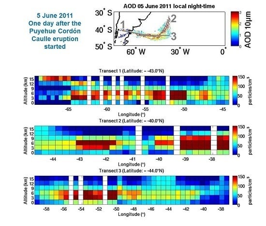
3.2. The Test Case: The Puyehue-Cordón Caulle Eruption in June 2011

The eruption studied in this work is a Plinian eruption from a fissure in the Puyehue-Cordón Caulle Volcanic Complex (2236 m altitude) in central Chile, which began on 4 June 2011 at 19:15 UTC (or 16:15 local time). This was an intense eruption, lasting for a few months. Following Bignami et al. [13], the initial explosion ejected ash in the air up to a 12.2-km altitude. They have also retrieved AOD and effective radius from measurements by MODIS onboard Aqua, using the brightness temperature difference technique, and the plume altitude using an interpolation between MODIS brightness temperature (BT) in the 11-μm band of the most opaque pixels and an atmospheric temperature profile. The geographic pattern of the plume on 5 June is very similar to the one we observe (as shown for example in Figure 6), with a 550-nm AOD of up to four. The effective radius obtained by Bignami et al. [13] is about 4 to 5 μm, remaining approximately constant with time during the first month after the beginning of the eruption. However, as mentioned previously, the MAPIR retrievals were of extremely poor quality with such big particles, while they were good with smaller particles. This issue is linked to the fact that the TIR signature of mineral aerosols depends on their physical parameters (refractive index and particle size) in addition to the effect of the particle concentration (or integrated AOD) and altitude distribution. Ideally, one would retrieve all of these parameters together. However in practice, this is impossible. Those parameters are not independent, and the signal does not contain enough information for a joint retrieval of vertical profiles, particle size and refractive index from each single spectrum. In MAPIR, we have set the focus on the vertical distribution and used a decent set of fixed aerosol physical parameters. This set has been selected because it led to converging retrievals. Additionally, the presence of ice clouds together with the ash particles makes the situation even more difficult. It is possible (even though impossible to confirm without retrieving information about ice particles) that the set of physical parameters that seems to suit our test case best is actually describing the ash/ice mixture.
The plume altitude was estimated by Bignami et al. [13] at about a 19-km altitude right after the eruption (but with an uncertainty of about 5 km) and quickly decreases to reach about a 7-km altitude on 7 June (with an uncertainty of about 2.5 km). However, our understanding is that this approach only allows the detection of one ash cloud. The given altitude is probably close to the top of the ash layer (with an effect of the cloud opacity).
Klüser et al. [31] studied this eruption by applying the IMARS algorithm to IASI observations, in terms of optical depth and, in a newer version, also ash emission altitude. These results will be used in Section 3.2.2 for comparisons. Additionally, they traced back the trajectory of the ash plume from the locations of IASI observations of this plume to the volcano, which revealed that there were two emission heights: between 3 and 7 km with a plume transported to the southeast and above 9 km with a plume transported to the east.
Figure 6. Retrieval results for 5 June 2011, local morning overpass. The plots show the retrieved ash aerosol optical depth (AOD) at 10 μm, the root mean square of the residuals (RMSR) in brightness temperature (BT) units (K) and the number of degrees of freedom (DOF). White spaces are locations where our ash pre-filter was not triggered; no retrieval was therefore undertaken. The black triangle represents the volcano (in the first panel, we have added an arrow pointing to that location, labeled PCC as the initials of the Puyehue Cordón Caulle). An insert in the RMSR plot shows a histogram of the values.
Remotesensing 08 00103 g006
It is interesting to mention that the Level 3 aerosol products for MODIS Collection 6 and MISR v31 at the location of the Puyehue ash plume contain mostly fill values, indicating that either the plume was detected as a cloud or that the retrieval failed. As studying these products is not the purpose of the work presented here, we did not go further into detail regarding the reasons for this. Nevertheless, it underlines the issues with the use of such instruments for studying very thick ash plumes mixed with ice, as is the case for the Puyehue eruption.

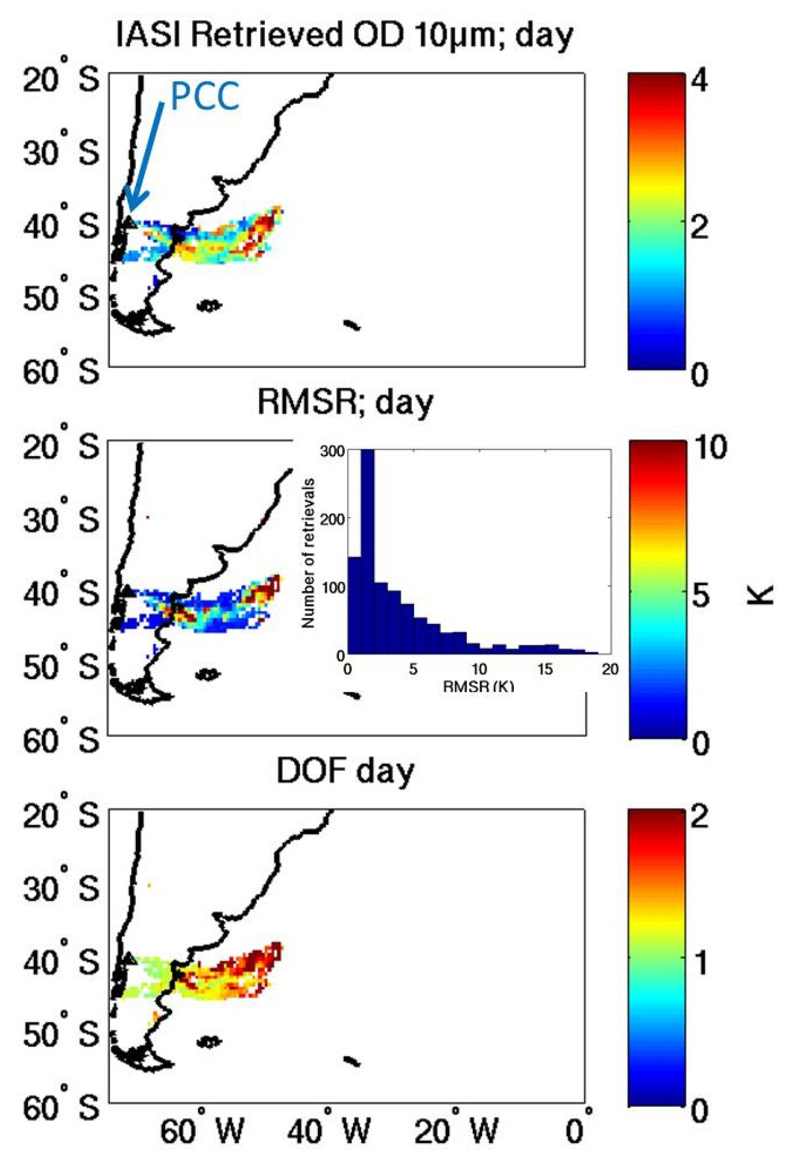
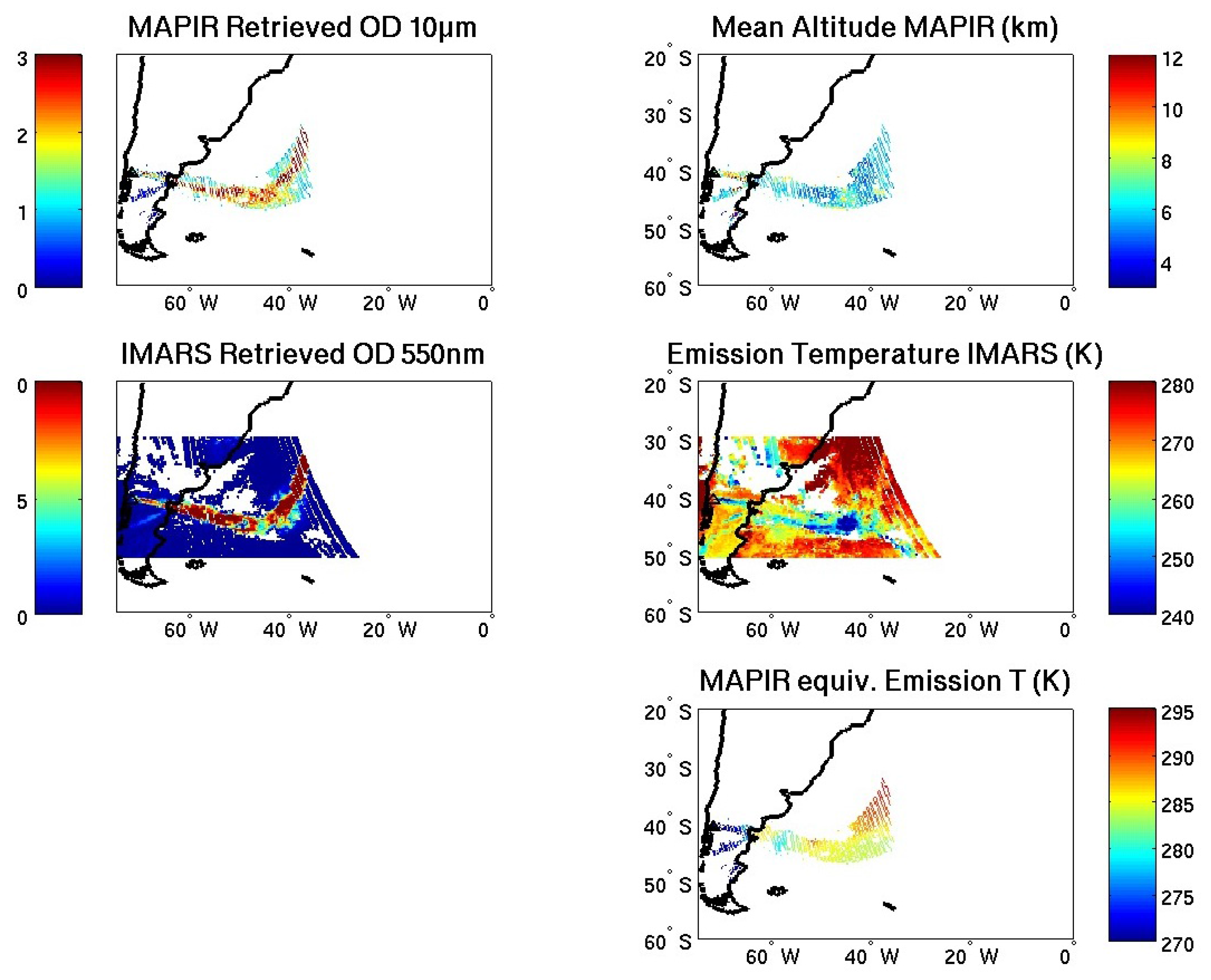
3.2.1. Detailed Analysis of Our Retrieval Results on the 5th of June

Figure 6 shows our retrieval results for the second overpass of IASI above the area of the Puyehue volcano after the eruption started (5 June 2011 at about 10:00 local time, 13:00 UTC). This is the first overpass for which the plume is geographically large enough for an analysis of the capabilities of our retrieval strategy. Indeed, for the first IASI overpass, only 6 h after the eruption, we only spot a few ashy spectra, quite scattered (not forming a real plume), mostly over Argentina going east from the volcano. Figure 6 shows the retrieved ash aerosol optical depth (AOD) at 10 μm, the root mean square of the residuals (RMSR) in BT units (K) and the number of degrees of freedom for the vertical profile retrieval (DOF). White spaces are locations where our ash pre-filter was not triggered; no retrieval was therefore undertaken. The first observation from those plots is that the retrieved 10 μm AOD is extremely high, as was also observed by Bignami et al. [13] reporting 550 nm ODs up to at least four. Even though one might argue that the 10 μm AOD does not contain the small particles’ contribution as does visible AOD, in this case, most of the ash particles are in the coarse mode, as shown by the effective size retrievals performed by Bignami et al. [13]. A conversion factor might therefore be obtained using a simple Mie code for computing the extinction at 10 μ m and at 550 nm using the PSD and refractive index used in this study (and with the spherical assumption, which might not be really good for visible wavelengths). This conversion factor is 1.67, the 550 nm AOD being higher. However, this conversion factor depends much more on the aerosol parametrization (refractive index and PSD) than the 10 μ m AOD does. For example, if the particle size is increased to an effective radius of 4 μ m, the 10 μ m AOD would vary by 10% at most, while the conversion to 550 nm would be divided by about a factor of two, depending also on the refractive index. As we have chosen a generic refractive index and a fixed particle size, the 10 μ m AOD reported is only slightly affected by uncertainties on those, while the conversion to 550 nm would be greatly affected by particle size and refractive index uncertainties. Therefore, we have decided not to convert the AOD to 550 nm and only provide an indicative conversion factor.
Our retrievals usually contain two degrees of freedom. This means that the six retrieved aerosol concentrations (at six altitudes) are not mutually independent; rather there are two independent partial columns. The two independent pieces of information do not always lie in the same altitude range. Therefore, it is impossible to determine in advance the altitude range that would match one piece of information.
The RMS of the retrievals is in most cases below 2 K, but increases up to more than 10 K at two places, for a limited number of retrievals, as shown in the insert containing a histogram, in Figure 6. At the coastline, the very high RMSR can be explained by the presence of quite a few ice particles, as seen in Figure 5, where an intense spectral signature of ice is detected. At the eastern part of the plume, the ice signature seems less intense. However, if looking at the IASI spectra in that area, selecting those for which the retrieval produced a RMSR higher than 10 K (Figure 7), the signature of a very thick ice cloud (as shown in Bantges et al. [52] or Clarisse et al. [28]) is present in the 800 to 850 cm - 1 spectral window. This signature is then overwhelmed by the extremely intense ash signature also clearly observed in the spectral window shown. It is this very intense ash signature that prevents our ice test from being triggered in most of those cases. Therefore, the high RMSR of our retrievals is explained by the presence of a thick ice cloud together with the extreme ash concentration. It is surprising that the ash retrievals do not fail under these conditions.
Figure 7. IASI measured spectra on 5 June, local morning overpass, in the area between 30 and 50 W, for which the ash retrievals were undertaken and resulted in a root mean square of residuals (RMSR) >10 K. Each line represents on single IASI spectrum.
Remotesensing 08 00103 g007
The strategy we have developed allows us to obtain, for the first time, vertical profiles of ash number concentration. A three-dimensional visualization on a two-dimensional plane is not always easy, and we have adopted three approaches here. The first one is to look at transects across the plume in different directions; the second one is to plot the concentration at each altitude separately; and the third one is to stack those plots to make it look like a 3D plot with perspective. The first option will be used here, to analyze the ash plume on the evening of the 5th of June, and the second and third options will be used to compare with IMARS results and show multiple days and follow the ash plume evolution.
Figure 8 shows three transects across the 5th June evening plume. The transects are computed with a step of 0.4 with averaging along 0.2 around the transect point. The first transect, which follows the southeast path from the volcano, clearly shows two distinct aerosol layers, at around 15 km close to the volcano and at around 3 to 6 km further east (at the southern part of the plume). For a small part of the transect, the two layers are observed together (in the same IASI scenes), underlining the ability of our algorithm to separate two aerosol layers. In order to support that statement, we also show a set of averaging kernels corresponding to a scene where we retrieve two aerosol layers (shown with a blue arrow in the first transect), with 1.6 degrees of freedom. Those averaging kernels clearly show sensitivity along the whole altitude range, but also a large vertical spread of the information as expected for nadir sensors. Most of the averaging kernels peak at the corresponding retrieval altitude, meaning that the retrieved concentration at each altitude comes mainly from the presence of aerosols at that altitude. However, a non-negligible contribution from the other altitudes is present. We cannot show averaging kernels for all possible situations, but we describe different possibilities and their implications. For most of the scenes, the situation is similar to the one shown in Figure 8. Then, there are scenes for which the averaging kernels show sensitivity only to a small part of the atmosphere (for example, two retrieval layers), even sometimes with two degrees of freedom. In those cases, only one distinct aerosol layer may be detected. Finally, there are scenes for which our retrievals provide two distinct aerosol layers, while there is only one degree of freedom. This does not mean that physically those two layers are incorrect, and in particular, in the case we have investigated, there was a high spatial coherence between those profiles and the other retrievals around them. It however means that the concentrations retrieved in these two aerosol layers are correlated, accounting together for only one piece of information.
Figure 8. Transects across different parts of the ash plume on 5 June 2011, local evening. The map at the top right shows the corresponding AOD map with the three transect locations. Averaging kernels are also shown for the IASI profile marked with a blue arrow in the first transect, for each retrieval altitude. The number of DOF for this scene was 1.6.
Remotesensing 08 00103 g008
The second transect crossing the plume from its southern part to the northeast and the third transect crossing the plume from west to east show mainly ash around a 3- to 6-km altitude and up to a 9-km altitude at the east of the plume. This is in agreement with the findings of Klüser et al. [31] based on trajectory simulations: the ash emitted between 3 and 7 km was transported to the southeast, and the ash emitted at altitudes above 9 km was transported to the east. The first transect profiles also agree with the detection of ash at quite high altitudes (up to respectively 19, 16, 14 km on the 4th, 5th and 6th of June) by Bignami et al. [13].

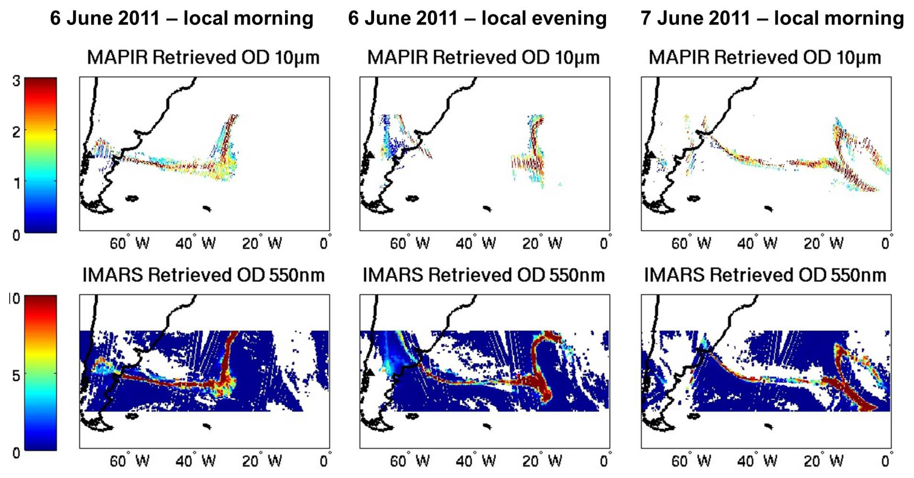
3.2.2. Comparison with the IMARS Product: 5 to 7 June 2011

The comparisons with results from the IMARS algorithm are two-fold. We first compare the AOD. The IMARS AOD was converted from TIR to 550 nm by using the ratio of extinction coefficients in TIR and at 550 nm [45,46]. This ratio is not constant, as IMARS uses a combination of minerals, which varies. As mentioned earlier, for the PSD and refractive index used in the MAPIR retrievals, the AOD factor from 10 μm to 550 nm would be 1.67, but it highly depends on the aerosol parameterization, as explained in Section 3.2.1; therefore, our AOD comparisons need to remain qualitative. The second part of the comparison concerns the altitude of the ash plume. In the IMARS algorithm, an emission temperature is retrieved, while MAPIR provides a vertical profile of number concentration, from which we have obtained a mean altitude for the ash plume (the altitude for which half the ash particles are below and half above). This concept of mean altitude may be irrelevant in the case of multiple aerosol layers, the mean altitude then possibly being the altitude at which there are no aerosols (i.e., one layer being above and the second layer being below the mean altitude). However, these cases are not so numerous in the studied plume. The link between emission temperature and altitude requires the knowledge of the atmospheric temperature vertical profile: we have used the IASI Level 2 operational product, which is also used in the MAPIR retrievals. An issue may arise from the fact that for the eruption studied in this work, ash went high enough in the air to cross the tropopause. Therefore, for some cases, an emission temperature could correspond to two different altitudes, below or above the tropopause. We have thus decided not to convert the IMARS emission temperature to an altitude, but to convert the MAPIR mean altitudes to an equivalent emission temperature. A second issue that might arise in those comparisons is the fact that the IMARS algorithm is based on different mineral refractive indices, while MAPIR is based on a single constant refractive index. Regarding the altitude-like information, the IMARS emission altitude is very sensitive to the single scattering albedo, which is varying with the combination of the different minerals, while again it is constant in the MAPIR algorithm. As mentioned earlier, it has been shown that the IMARS scheme is expected to overestimate the emission temperature because of the Mie treatment [46].
Figure 9 shows, for the 5th of June 2011 local evening, the 10 μm AOD and mean aerosol altitude from MAPIR, the AOD converted at 550 nm and the emission temperature from IMARS, as well as the emission temperature equivalent to the MAPIR mean altitude. Looking at the two sets of AOD, the first clear observation is that both algorithms spot ash at the same place, with the same geographical patterns. This is quite remarkable for two algorithms working with very different assumptions and mathematical approaches.
To analyze the emission temperatures, let us first provide the surface and atmospheric temperatures for that particular day at the plume location, respectively from ECMWF and IASI Level 2 data (the data used in MAPIR retrievals). The surface temperature is about 270 K above land and 285 to 290 K above sea. The atmospheric temperatures at 0 to 18 km by 3-km steps are, on average, within the ash plume: 274 K, 259 K, 241 K, 220 K, 217 K, 219 K, 216 K. The MAPIR emission temperatures are, within the plume, of the order of 230 to 250 K, corresponding to the mean altitudes of about 6 to 8 km. The IMARS emission temperatures are of the order of 240 to 265 K within the plume, with a geographical pattern matching that of our equivalent emission temperatures, but about 10 to 15 K higher. These temperatures cannot correspond to altitudes above the tropopause and are therefore linked to altitudes of 3 to 6 km. Considering all of the other altitude information that we already mentioned, it is most likely that the IMARS retrieval tends to overestimate the emission temperature, as was expected (see the earlier remarks). Nevertheless, this cannot be regarded as final proof for the validity of the MAPIR altitudes; therefore, a comparison with active remote sensing data is absolutely necessary (see Section 3.2.3). The results for the next three overpasses lead to the same conclusions: the IMARS emission temperature is higher than the MAPIR equivalent emission temperatures by 10 to 30 K. The AOD comparison for the following overpasses (Figure 10) clearly illustrates the plume transport and shows that two very different algorithms provide similar results for the ash plume of the Puyehue eruption.
Figure 9. Comparison between MAPIR (presented in this paper) and IMARS (updated from [31]) for the 5 June 2011, local evening. The retrievals are presented in terms of AOD and mean altitude information (in the form of emission temperature for the IMARS product).
Remotesensing 08 00103 g009
Figure 10. Same as Figure 9, left part, for the 6 June 2011 local morning (left) to the 7 June local morning (right).
Remotesensing 08 00103 g010

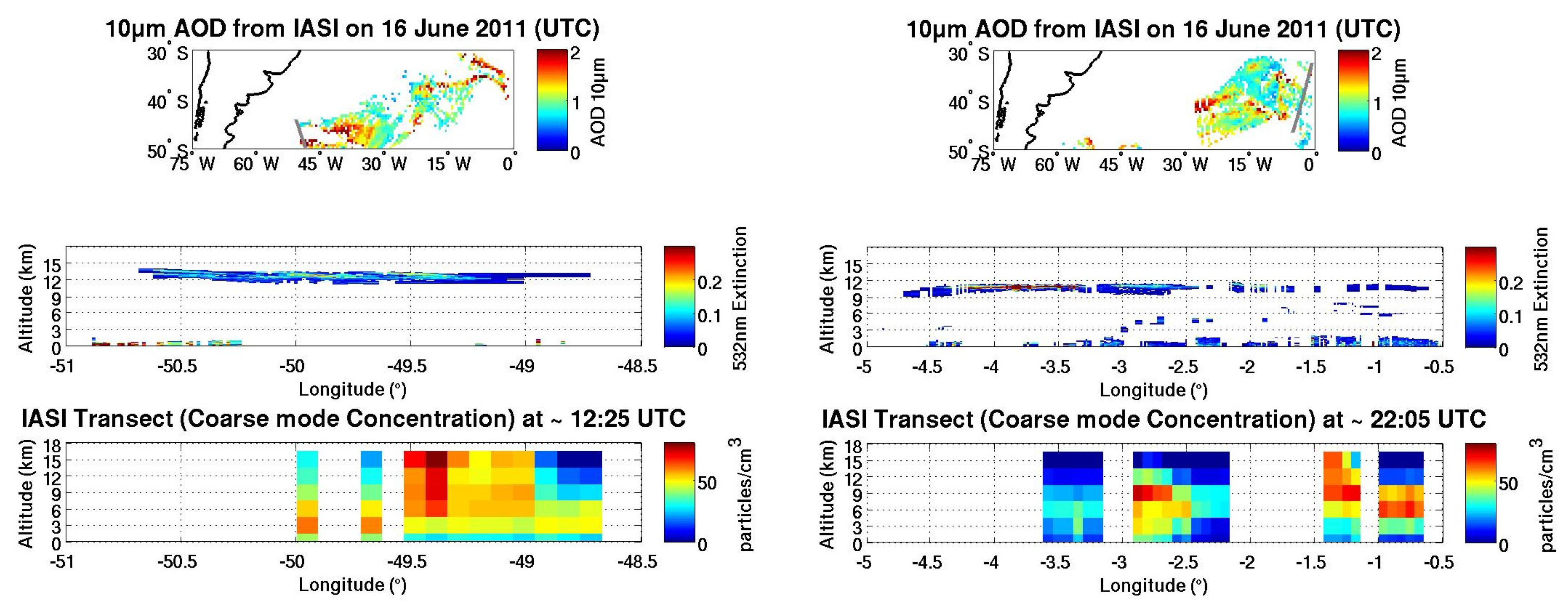
3.2.3. Comparison with CALIOP High Resolution Vertical Profiles: 16 June 2011

We have already compared our altitude information to what is available in the literature and shown that our retrieval results are reasonable in terms of altitude. However, to try to validate the vertical profiles, the use of CALIOP data is essential. The CALIOP instrument was (quite unfortunate for this study) out of service at the time of the eruption. It came back to operation on the 16th of June, more than 10 days after the initial eruption. We will use that day for comparisons.
Figure 11 shows comparisons of our results with CALIOP extinction measurements, for one CALIOP day-time track and one CALIOP night-time track. The comparison of the absolute value of the extinction versus concentration will not be done. Even though it is possible to estimate a factor from Mie computations as explained in Section 2.2.2, the main goal here is to compare our retrieved altitude information to the best available altitude information from another sensor. In addition, when comparing the IASI retrieval results with CALIOP measurements, one should be aware of the inherent time difference of about 3 to 6 h (depending if the CALIOP track falls in the west or east part of the IASI swath). During that time, the aerosols may have moved. The comparisons may be especially sensitive to this because CALIOP data are recorded along a very thin track and do therefore not provide a complete picture of the plume. For that reason, we constructed the IASI transects as follows: each 0.25 along the transect, a vertical profile is obtained as the mean of all of the IASI retrievals within 100 km of that point. An additional difficulty for the comparison is that the CALIOP product contains different types of aerosols with an aerosol type characterization flag, but currently, there does not exist an ash-type aerosol, and the discrimination must therefore be done “by the expert’s eye”. Finally, while CALIOP provides extinction with extremely high vertical resolution, our retrievals have a vertical resolution of 3 km.
For the day-time comparison (Figure 11, left), CALIOP sees a thin ash layer at a 12-km to a 14-km altitude, with a low extinction. In our IASI retrieval results along this CALIOP track, we see the peak ash concentration at that altitude (12 to 15 km), but also some ash lower in the troposphere, down to a 6-km altitude. The white places in our MAPIR results are mainly where the aerosol pre-filter was not triggered (and some that did not pass the pre-quality checks on ancillary data). The CALIOP aerosol layer very close to the surface is most probably marine aerosols. It is quite peculiar that this layer of marine aerosols is not seen from 50 to 49 W, while it is almost always observed above seas. This could, without any certainty, be an indication that CALIOP could not see under the ash layer. However, the extinction does not seem to be high enough to explain that. The two other CALIOP tracks crossing the plume during that day fall one right in the area between the two parts of the plume seen by IASI and the second at the east end of the plume. For the first one, the CALIOP track contains an extinction layer around 12 to 9 km, while ash is not detected by IASI. For the second one, high ash concentration is detected by IASI at about a 6-km altitude, and nothing is seen by CALIOP. Both can be explained by the plume’s movement during the time between the IASI and CALIOP overpass. Indeed, the plume seems to be moving fast considering the significant difference between the retrieval results during day-time and night-time (Figure 11).
Figure 11. Comparison between CALIOP transects (middle panel) across the ash plume on 16 June 2011 and the IASI retrievals along those transects (lower panel). The optical depths are also shown in the upper panel. The left part concerns day-time data, while the right part concerns night-time data.
Remotesensing 08 00103 g011
For the night-time comparisons (Figure 11, right), CALIOP data show again a continuous extinction between a 9- and 12-km altitude, with also some extinction between a 3- and 6-km altitude and the usual marine aerosols close to the surface. Our retrievals also clearly show the peak ash concentration around a 9-km altitude, with some ash underneath. The second CALIOP overpass of the plume during that night occurs right at the west part of the IASI observed plume (at a location where we do not have IASI data) showing a high extinction layer at around a 12- to 15-km altitude.
We have seen that the track to track comparisons between IASI and CALIOP are quite difficult to undertake considering the significant time difference and the very limited geographical coverage by CALIOP. Another approach might be to look at the “general trend” in the two datasets, regarding the plume altitude. On the 16th of June, CALIOP shows mainly an ash layer at a 12- to 15-km altitude in the west part of the plume, going down to a 9- to 12-km altitude towards the east part of the plume. Looking at the concentrations at each retrieval altitude for that day in Figure 12, ash is detected in the western part of the plume up to a 15-km altitude, but also at some point locations in the east part of the plume. All along the plume, ash is observed at a 6-km altitude and often in the two adjacent layers (3 and 9 km). It would therefore seem that our retrievals underestimate the ash plume altitude with respect to CALIOP measurements. However, Bignami et al. [13] reported a plume altitude of about 6 km for that period, which is the altitude at which we also find most of the ash.
Figure 12. Ash concentration at the different retrieval altitudes for 16 June 2011.
Remotesensing 08 00103 g012

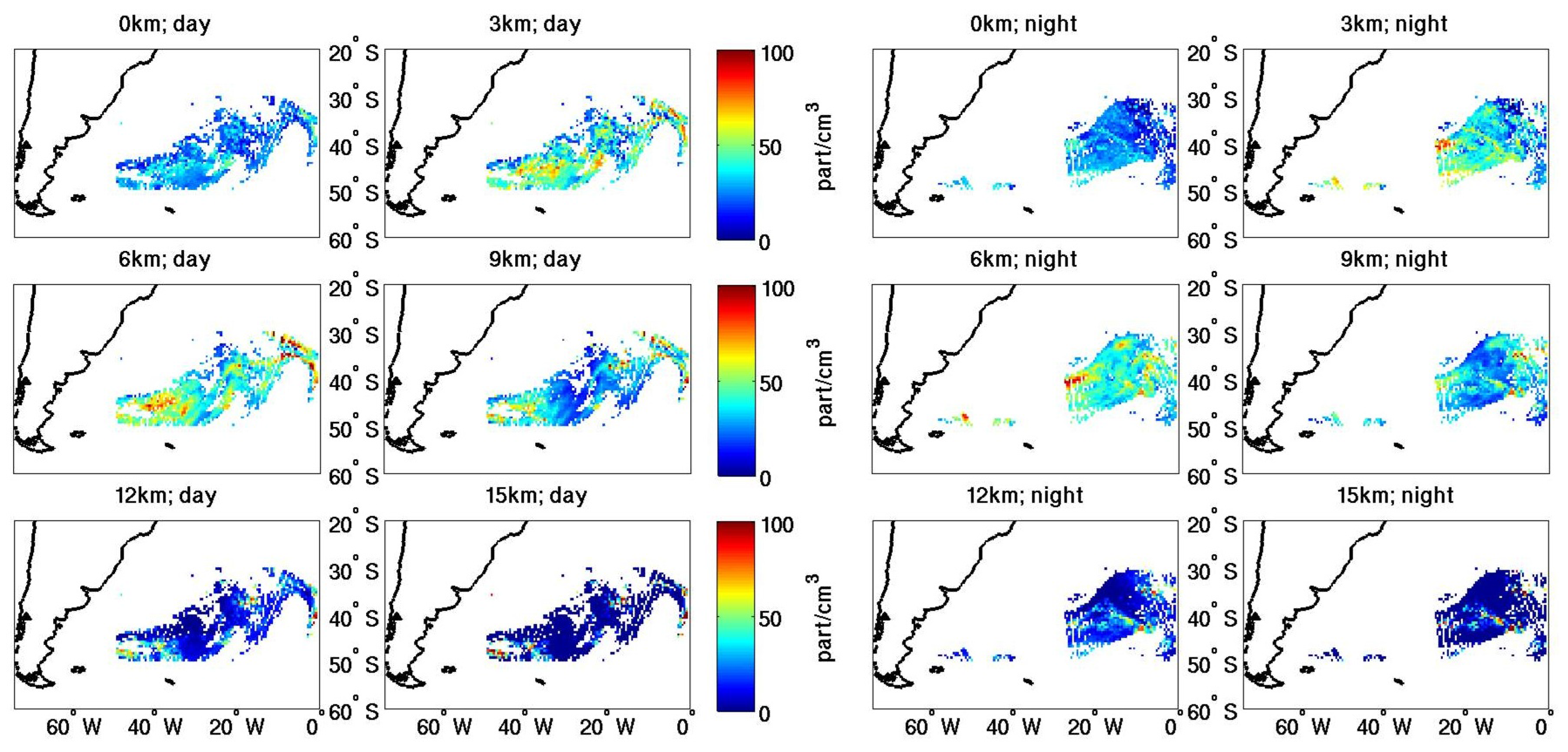
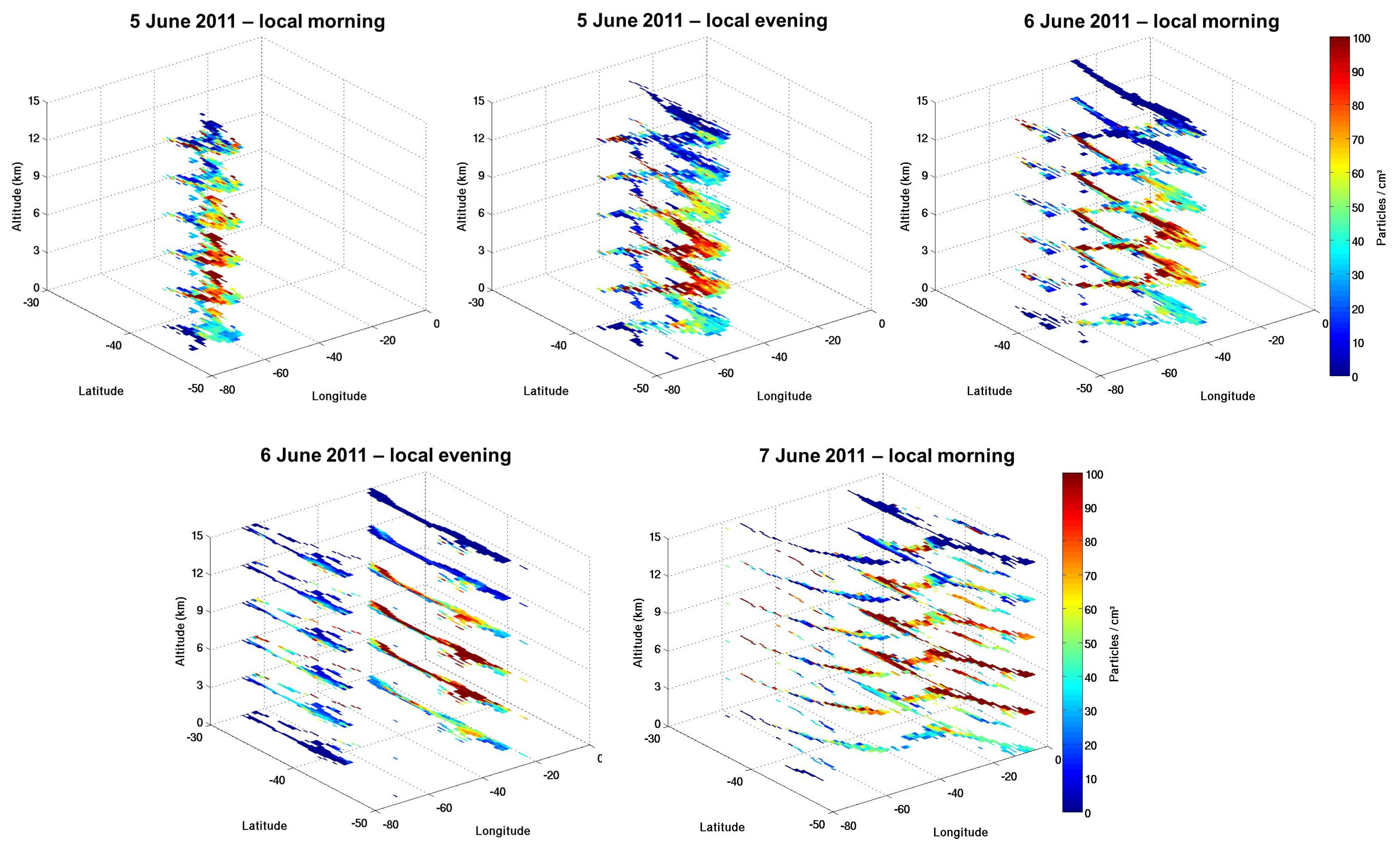
3.2.4. Retrieval Results Analysis: Full 3D View of the Plume from 5 to 7 June 2011

Figure 13 shows the 3D distribution of the Puyehue plume for 5 to 7 June. Most of the ash seems to be between a 3- and 9-km altitude for the west part of the plume. At the eastern part of the plume, it spreads north with more ash at a 9- to 12-km altitude. This last part of the plume probably corresponds to the beginning of the eruption, when the explosion ejected ash higher up in the atmosphere. The western part of the plume most probably corresponds to the almost continuous ash ejections during the first two days (indeed, ash is observed above the volcano until 6 June), occurring at lower altitudes than the first explosive event. Almost no ash is detected in the first vertical layer, close to the surface, during these first three days after the eruption, and the ash altitudes do not seem to really change with time (ash is transported at an almost constant altitude). This means that the deposition did not yet even start after three days and that most probably ash will stay a long time in the atmosphere. This was indeed the case: Bignami et al. [13] reported the presence of ash at least one month after the eruption, still at a mean altitude of about 5 km.
Figure 13. 3D view of the ash plume from 5 to 7 June 2011.
Remotesensing 08 00103 g013

4. Conclusions

Volcanic ash is an important actor in the climate system and a major threat to aviation and to health when close to the surface. There is to the authors’ knowledge at the moment no method that allows the retrieval of a four-dimensional distribution of volcanic ash in the atmosphere, with good spatial and time coverage. The method detailed in this work allows the retrieval of vertical profiles of volcanic ash number concentration from IASI thermal infrared measurements, with almost global coverage twice a day. The method is based on the optimal estimation formalism, and the retrievals contain two degrees of freedom (two independent partial columns), allowing up to two separate ash layers to be distinguished. There is significant vertical smearing of the aerosol concentration, which is usual for profiles retrieved from nadir measurements.
The retrieval strategy has been applied to study the eruption from the Puyehue-Cordón Caulle that started on the 4th of June 2011. During this eruption, parts of the ash plume were mixed with ice particles, making the ash retrievals more difficult. We have compared our results with other published studies of the same eruption, with data from a different algorithm providing ash optical depth from IASI measurements and with CALIOP high resolution vertical extinction measurements. All of these comparisons lead to the conclusion that, even though it is not possible to completely validate it, our method provides a reasonable 3D distribution of the ash plume.
This work opens the door to the availability of a 3D distribution of volcanic ash with global coverage twice a day, which would greatly enhance the way air traffic is modified in case of strong eruptions. Indeed, the knowledge of the ash plume height could allow flights to pass at the geographic location of the plume if their altitude is different enough from the plume’s altitude. Additionally, the climate effects of volcanic ash would be better evaluated if not only the optical depth, but also the altitude of the different ash clouds is known. However, there are still a series of issues that have to be addressed before reaching the state of operational ash monitoring with the algorithm developed here. First, it is not yet clear that all eruptions could be studied by this method. If the surface is extremely cold and the atmospheric temperature varies too little with altitude, the altitude sensitivity would drastically decrease and our retrievals (as currently designed) would probably fail. Second, ash from each eruption has different properties (composition, size), making it quite difficult to generalize. We can accept to work with a generic refractive index, as was done here, but this could fail for some plumes with a very different composition. The particle size is also an important parameter. Finally, the problem of ice mixed with ash should be solved, in order to avoid the high uncertainty linked to the fact that those two aerosol types have opposite effects in the thermal infrared. To solve that problem, a retrieval of two aerosol types together should be designed. This is technically feasible in MAPIR, but requires proper additional scientific developments.

Acknowledgments

Sophie Vandenbussche acknowledges the Belgian Science Policy supplementary researcher program, the Belgian Science Policy/ESA A3C PRODEX program, the Solar Terrestrial Center of Excellence and the ESA aerosols CCI Phase 2 project for funding the research on desert dust aerosols, on which this work has built. Kwinten Maes acknowledges Ghent University for providing support for a master’s thesis that lead to the results contained in this publication. Lars Klüser acknowledges the ESA aerosols CCI Phase 2 project. The authors acknowledge Ann Carine Vandaele and Svetlana Kochenova for their work on the ASIMUT retrieval algorithm and its link to the radiative transfer code LIDORT. The authors acknowledge the Belgian Institute for Space Aeronomy ICT team for their support.

Author Contributions

Kwinten Maes and Sophie Vandenbussche established the retrieval strategy, studied the test case and wrote most of the paper. Lars Klüser provided the improved version of the IMARS dataset, wrote parts of the paper and participated in the discussion of all results. Nicolas Kumps was in charge of extracting all of the IASI and associated datasets needed for this work. Martine de Mazière supervised the whole project.

Conflicts of Interest

The authors declare no conflict of interest.

References

  1. Swanson, S.E.; Beget, J. Melting properties of volcanic ash. In Proceedings of the First International Symposium on Volcanic Ash and Aviation Safety, Seattle, DC, USA, 8–12 July 1991; pp. 87–92.
  2. Miller, T.P.; Casadevall, T. Volcanic ash hazards to aviation. In Encyclopedia of Volcanoes; Sigurdsson, H., Ed.; Academic Press: San Diego, CA, USA, 2000; pp. 915–930. [Google Scholar]
  3. Prata, A. Satellite detection of hazardous volcanic clouds and the risk to global air traffic. Nat. Hazards 2009, 51, 303–324. [Google Scholar] [CrossRef]
  4. Zehner, C. Monitoring volcanic ash from space. In Proceedings of the ESA-EUMETSAT Workshop, Eyjafjöll Volcano, Iceland, 14 April–23 May 2010. [CrossRef]
  5. Haywood, J.; Boucher, O. Estimates of the direct and indirect radiative forcing due to tropospheric aerosols: A review. Rev. Geophys. 2000, 38, 513–543. [Google Scholar] [CrossRef]
  6. Langmann, B. Volcanic ash versus mineral dust: Atmospheric processing and environmental and climate impacts. ISRN Atmos. Sci. 2013, 2013, 245076. [Google Scholar] [CrossRef]
  7. Ramanathan, A.; Crutzen, P.J.; Kiehl, J.T.; Rosenfeld, D. Aerosols, climate, and the hydrological cycle. Science 2001, 294, 2119–2124. [Google Scholar] [CrossRef] [PubMed]
  8. Stevens, B.; Feingold, G. Untangling aerosol effects on clouds and precipitation in a buffered system. Nature 2009, 461, 607–613. [Google Scholar] [CrossRef] [PubMed]
  9. Myhre, G.; Shindell, D.; Bréon, F.M.; Collins, W.; Fuglestvedt, J.; Huang, J.; Koch, D.; Lamarque, J.F.; Lee, D.; Mendoza, B.; et al. Anthropogenic and natural radiative forcing. In Climate Change 2013: The Physical Science Basis; Stocker, T.F., Qin, D., Plattner, G.-K., Tignor, M., Allen, S.K., Boschung, J., Nauels, A., Xia, Y., Bex, V., Midgley, P.M., Eds.; Cambridge University Press: Cambridge, UK; New York, NY, USA, 2013; Chapter 8; pp. 659–740. [Google Scholar]
  10. Western, L.M.; Watson, M.I.; Francis, P.N. Uncertainty in two-channel infrared remote sensing retrievals of a well-characterised volcanic ash cloud. Bull. Volcanol. 2015, 77. [Google Scholar] [CrossRef]
  11. Naeger, A.R.; Christopher, S.A. The identification and tracking of volcanic ash using the Meteosat Second Generation (MSG) Spinning Enhanced Visible and Infrared Imager (SEVIRI). Atmos. Meas. Tech. 2014, 7, 581–597. [Google Scholar] [CrossRef]
  12. Dubuisson, P.; Herbin, H.; Minvielle, F.; Compiègne, M.; Thieuleux, F.; Parol, F.; Pelon, J. Remote sensing of volcanic ash plumes from thermal infrared: A case study analysis from SEVIRI, MODIS and IASI instruments. Atmos. Meas. Tech. 2014, 7, 359–371. [Google Scholar] [CrossRef] [Green Version]
  13. Bignami, C.; Corradini, S.; Merucci, L.; de Michele, M.; Raucoules, D.; de Astis, G.; Stramondo, S.; Piedra, J. Multisensor satellite monitoring of the 2011 Puyehue-Cordon Caulle eruption. IEEE J. Sel. Top. Appl. Earth Obs. Remote Sens. 2014, 7, 2786–2796. [Google Scholar] [CrossRef]
  14. Wiegner, M.; Gasteiger, J.; Gross, S.; Schnell, F.; Freudenthaler, V.; Forkel, R. Characterization of the Eyjafjallajökull ash-plume: Potential of LiDAR remote sensing. Phys. Chem. Earth. A/B/C 2012, 45–46, 79–86. [Google Scholar] [CrossRef]
  15. Prata, A.J.; Prata, A.T. Eyjafjallajökull volcanic ash concentrations determined using Spin Enhanced Visible and Infrared Imager measurements. J. Geophys. Res.: Atmos. 2012, 117, D00U23. [Google Scholar] [CrossRef]
  16. Wen, S.; Rose, W.I. Retrieval of sizes and total masses of particles in volcanic clouds using AVHRR bands 4 and 5. J. Geophys. Res.: Atmos. 1994, 99, 5421–5431. [Google Scholar] [CrossRef]
  17. Sears, T.M.; Thomas, G.E.; Carboni, E.; Smith, A.J.; Grainger, R.G. SO2 as a possible proxy for volcanic ash in aviation hazard avoidance. J. Geophys. Res.: Atmos. 2013, 118, 5698–5709. [Google Scholar]
  18. Brenot, H.; Theys, N.; Clarisse, L.; van Geffen, J.; van Gent, J.; van Roozendael, M.; van der, A.R.; Hurtmans, D.; Coheur, P.F.; Clerbaux, C.; et al. Support to Aviation Control Service (SACS): An online service for near-real-time satellite monitoring of volcanic plumes. Nat. Hazards Earth Syst. Sci. 2014, 14, 1099–1123. [Google Scholar] [CrossRef] [Green Version]
  19. Karagulian, F.; Clarisse, L.; Clerbaux, C.; Prata, A.J.; Hurtmans, D.; Coheur, P.F. Detection of volcanic SO2, ash, and H2SO4 using the Infrared Atmospheric Sounding Interferometer (IASI). J. Geophys. Res.: Atmos. 2010, 115, D00L02. [Google Scholar]
  20. Francis, P.N.; Cooke, M.C.; Saunders, R.W. Retrieval of physical properties of volcanic ash using Meteosat: A case study from the 2010 Eyjafjallajokull eruption. J. Geophys. Res.: Atmos. 2012, 117, D00U09. [Google Scholar] [CrossRef]
  21. Carboni, E.; Grainger, R.; Walker, J.; Dudhia, A.; Siddans, R. A new scheme for sulphur dioxide retrieval from IASI measurements: Application to the Eyjafjallajokull eruption of April and May 2010. Atmos. Chem. Phys. 2012, 12, 11417–11434. [Google Scholar] [CrossRef] [Green Version]
  22. Theys, N.; Campion, R.; Clarisse, L.; Brenot, H.; van Gent, J.; Dils, B.; Corradini, S.; Merucci, L.; Coheur, P.F.; van Roozendael, M.; et al. Volcanic SO2 fluxes derived from satellite data: A survey using OMI, GOME-2, IASI and MODIS. Atmos. Chem. Phys. 2013, 13, 5945–5968. [Google Scholar] [CrossRef] [Green Version]
  23. Zakšek, K.; Hort, M.; Zaletelj, J.; Langmann, B. Monitoring volcanic ash cloud top height through simultaneous retrieval of optical data from polar orbiting and geostationary satellites. Atmos. TChem. Phys. 2013, 13, 2589–2606. [Google Scholar] [CrossRef]
  24. Clarisse, L.; Coheur, P.F.; Theys, N.; Hurtmans, D.; Clerbaux, C. The 2011 Nabro eruption, a SO2 plume height analysis using IASI measurements. Atmos. Chem. Phys. 2014, 14, 3095–3111. [Google Scholar] [CrossRef]
  25. Ebmeier, S.K.; Sayer, A.M.; Grainger, R.G.; Mather, T.A.; Carboni, E. Systematic satellite observations of the impact of aerosols from passive volcanic degassing on local cloud properties. Atmos. Chem. Phys. 2014, 14, 10601–10618. [Google Scholar] [CrossRef]
  26. Winker, D.M.; Vaughan, M.A.; Omar, A.; Hu, Y.; Powell, K.A.; Liu, Z.; Hunt, W.H.; Young, S.A. Overview of the CALIPSO mission and CALIOP data processing algorithms. J. Atmos. Oceanic Technol. 2009, 26, 2310–2323. [Google Scholar] [CrossRef]
  27. Clerbaux, C.; Boynard, A.; Clarisse, L.; George, M.; Hadji-Lazaro, J.; Herbin, H.; Hurtmans, D.; Pommier, M.; Razavi, A.; Turquety, S.; et al. Monitoring of atmospheric composition using the thermal infrared IASI/MetOp sounder. Atmos. Chem. Phys. 2009, 9, 6041–6054. [Google Scholar] [CrossRef] [Green Version]
  28. Clarisse, L.; Hurtmans, D.; Prata, A.J.; Karagulian, F.; Clerbaux, C.; de Mazière, M.; Coheur, P.F. Retrieving radius, concentration, optical depth, and mass of different types of aerosols from high-resolution infrared nadir spectra. Appl. Opt. 2010, 49, 3713–3722. [Google Scholar] [CrossRef] [PubMed]
  29. Clarisse, L.; Coheur, P.F.; Prata, F.; Hadji-Lazaro, J.; Hurtmans, D.; Clerbaux, C. A unified approach to infrared aerosol remote sensing and type specification. Atmos. Chem. Phys. 2013, 13, 2195–2221. [Google Scholar] [CrossRef] [Green Version]
  30. Rodgers, C.D. Inverse Methods for Atmospheric Sounding—Theory and Practice; World Scientific: Singapore, 2000; Volume 2. [Google Scholar]
  31. Klüser, L.; Erbertseder, T.; Meyer-Arnek, J. Observation of volcanic ash from Puyehue-Cordón Caulle with IASI. Atmos. Meas. Tech. Discuss. 2012, 5, 4249–4283. [Google Scholar] [CrossRef]
  32. Vandenbussche, S.; Kochenova, S.; Vandaele, A.C.; Kumps, N.; de Mazière, M. Retrieval of desert dust aerosol vertical profiles from IASI measurements in the TIR atmospheric window. Atmos. Meas. Tech. 2013, 6, 2577–2591. [Google Scholar] [CrossRef]
  33. Vandaele, A.C.; de Mazière, M.; Drummond, R.; Mahieux, A.; Neefs, E.; Wilquet, V.; Korablev, O.; Fedorova, A.; Belyaev, D.; Montmessin, F.; et al. Composition of the Venus mesosphere measured by Solar Occultation at Infrared on board Venus Express. J. Geophys. Res. 2008, 113, E00B23. [Google Scholar] [CrossRef]
  34. Spurr, R. LIDORT and VLIDORT: Linearized pseudo-spherical scalar and vector discrete ordinate radiative transfer models for use in remote sensing retrieval problems. In Light Scattering Reviews 3; Kokhanovsky, A.A., Ed.; Springer: Berlin/Heidelberg, Germany, 2008; pp. 229–275. [Google Scholar]
  35. Mishchenko, M.I.; Dlugach, J.M.; Yanovitskij, E.G.; Zakharova, N.T. Bidirectional reflectance of flat, optically thick particulate layers: An efficient radiative transfer solution and applications to snow and soil surfaces. J. Quant. Spectrosc. Radiat. Transf. 1999, 63, 409–432. [Google Scholar] [CrossRef]
  36. Massie, S. Indices of refraction for the Hitran compilation. J. Quant. Spectrosc. Radiat. Transf. 1994, 52, 501–513. [Google Scholar] [CrossRef]
  37. Massie, S.; Goldman, A. The infrared absorption cross-section and refractive-index data in HITRAN. J. Quant. Spectrosc. Radiat. Transf. 2003, 82, 413–428. [Google Scholar] [CrossRef]
  38. Volz, F. Infrared refractive index of atmospheric aerosol substances. Appl. Opt. 1972, 11, 755–759. [Google Scholar] [CrossRef] [PubMed]
  39. Volz, F.E. Infrared optical constants of ammonium sulfate, sahara dust, volcanic pumice, and flyash. Appl. Opt. 1973, 12, 564–568. [Google Scholar] [CrossRef] [PubMed]
  40. Shettle, E.P.; Fenn, R.W. Models for the Aerosols of the Lower Atmosphere and the Effects of Humidity Variations on Their Optical Properties; AFGL-TR-79-0214; Optical Physics Division, Air Force Geophysics Laboratory: Hanscom AFB, MA, USA, 1979. [Google Scholar]
  41. Pollack, J.B.; Toon, O.B.; Khare, B.N. Optical properties of some terrestrial rocks and glasses. ICARUS 1973, 19, 372–389. [Google Scholar] [CrossRef]
  42. Pierangelo, C.; Mishchenko, M.; Balkanski, Y.; Chédin, A. Retrieving the effective radius of Saharan dust coarse mode from AIRS. Geophys. Res. Lett. 2005, 32, L20813. [Google Scholar] [CrossRef]
  43. DeSouza-Machado, S.G.; Strow, L.L.; Imbiriba, B.; McCann, K.; Hoff, R.M.; Hannon, S.E.; Martins, J.V.; Tanré, D.; Deuzé, J.L.; Ducos, F.; et al. Infrared retrievals of dust using AIRS: Comparisons of optical depths and heights derived for a North African dust storm to other collocated EOS A-Train and surface observations. J. Geophys. Res. 2010, 115, D15201. [Google Scholar] [CrossRef]
  44. Singer, B.; Jicha, B.; Harper, M.; Naranjo, J.; Lara, L.; Moreno-Roa, H. Eruptive history, geochronology, and magmatic evolution of the Puyehue-Cordón Caulle volcanic complex, Chile. Geol. Soc. Am. Bull. 2008, 120, 599–618. [Google Scholar] [CrossRef]
  45. Klüser, L.; Martynenko, D.; Holzer-Popp, T. Thermal infrared remote sensing of mineral dust over land and ocean: A spectral SVD based retrieval approach for IASI. Atmos. Meas. Tech. 2011, 4, 757–773. [Google Scholar] [CrossRef]
  46. Klüser, L.; Banks, J.; Martynenko, D.; Bergemann, C.; Brindley, H.; Holzer-Popp, T. Information content of space-borne hyperspectral infrared observations with respect to mineral dust properties. Remote Sens. Environ. 2015, 156, 294–309. [Google Scholar] [CrossRef]
  47. Newman, S.M.; Smith, J.A.; Glew, M.D.; Rogers, S.M.; Taylor, J.P. Temperature and salinity dependence of sea surface emissivity in the thermal infrared. Q. J. R. Meteorol. Soc. 2005, 131, 2539–2557. [Google Scholar] [CrossRef]
  48. Zhou, D.; Larar, A.; Liu, X.; Smith, W.; Strow, L.; Yang, P.; Schlussel, P.; Calbet, X. Global Land Surface Emissivity Retrieved From Satellite Ultraspectral IR Measurements. IEEE Trans. Geosci. Remote Sens. 2011, 49, 1277–1290. [Google Scholar] [CrossRef]
  49. August, T.; Klaes, D.; Schlüssel, P.; Hultberg, T.; Crapeau, M.; Arriaga, A.; O’Carroll, A.; Coppens, D.; Munro, R.; Calbet, X. IASI on MetOp-A: Operational Level 2 retrievals after five years in orbit. J. Quant. Spectrosc. Radiat. Transf. 2012, 113, 1340–1371. [Google Scholar] [CrossRef]
  50. Anderson, G.P.; Clough, S.A.; Kneizys, F.; Chetwynd, J.H.; Shettle, E.P. AFGL Atmospheric Constituent Profiles (0–120 km); Environmental Research Papers No. 954; Air Force Geophysics Laboratory: Hanscom AFB, MA, USA, 1986. [Google Scholar]
  51. Pavolonis, M.J.; Heidinger, A.K.; Sieglaff, J. Automated retrievals of volcanic ash and dust cloud properties from upwelling infrared measurements. J. Geophys. Res.: Atmos. 2013, 118, 1–23. [Google Scholar] [CrossRef]
  52. Bantges, R.; Russell, J.; Haigh, J. Cirrus cloud top-of-atmosphere radiance spectra in the thermal infrared. J. Quant. Spectrosc. Radiat. Transf. 1999, 63, 487–498. [Google Scholar] [CrossRef]

