Article

Mapping Deforestation in North Korea Using Phenology-Based Multi-Index and Random Forest

1
Interdisciplinary Program in Landscape Architecture, Seoul National University, Seoul 151-743, Korea
2
Department of Landscape Architecture and Rural System Engineering, Seoul National University, Seoul 151-743, Korea
3
Department of Environmental Science, Policy, and Management, University of California, Berkeley, CA 94720, USA
4
Plant Resources Division, National Institute of Biological Resources, Incheon 22689, Korea
*
Authors to whom correspondence should be addressed.
Remote Sens. 2016, 8(12), 997; https://doi.org/10.3390/rs8120997
Submission received: 26 August 2016 / Revised: 25 November 2016 / Accepted: 29 November 2016 / Published: 3 December 2016

Abstract

:
Phenology-based multi-index with the random forest (RF) algorithm can be used to overcome the shortcomings of traditional deforestation mapping that involves pixel-based classification, such as ISODATA or decision trees, and single images. The purpose of this study was to investigate methods to identify specific types of deforestation in North Korea, and to increase the accuracy of classification, using phenological characteristics extracted with multi-index and random forest algorithms. The mapping of deforestation area based on RF was carried out by merging phenology-based multi-indices (i.e., normalized difference vegetation index (NDVI), normalized difference water index (NDWI), and normalized difference soil index (NDSI)) derived from MODIS (Moderate Resolution Imaging Spectroradiometer) products and topographical variables. Our results showed overall classification accuracy of 89.38%, with corresponding kappa coefficients of 0.87. In particular, for forest and farm land categories with similar phenological characteristic (e.g., paddy, plateau vegetation, unstocked forest, hillside field), this approach improved the classification accuracy in comparison with pixel-based methods and other classes. The deforestation types were identified by incorporating point data from high-resolution imagery, outcomes of image classification, and slope data. Our study demonstrated that the proposed methodology could be used for deciding on the restoration priority and monitoring the expansion of deforestation areas.

Graphical Abstract

1. Introduction

Forest ecosystems provide ecological benefits to both humans and wildlife [1]. Growing global demand for food and fiber is accelerating the pressure on forest ecosystems around the world, from agriculture and logging [2]. These pressures have strong impacts on forest ecosystems, which include direct damage to remaining trees, as well as changes in plant and animal species diversity through destruction of the soil cover vegetation [1,3].
North Korea (the Democratic People’s Republic of Korea, DPRK) is known to have some of the most degraded forests in the world. Between 1990 and 2015, almost 40 percent of the forests in North Korea have either been converted to fields for food crop production, or cut down for fuel wood. This wide-spread deforestation has led to increased damage by natural disasters [4,5,6]. The characteristic forest landscape in North Korea is complex and heterogeneous; the major landscape types in the forest are hillside farm, unstocked forest, natural forest, and plateau vegetation. Deforestation of the forest landscape has been caused mostly by shifting cultivation practices and natural hazards in North Korea. This has affected nutrient loss from the soil in the forests and under other vegetation. To provide systematic, prioritized restoration efforts to address these problems, it is important to have a classification system for typical kinds of deforestation [7].
Remote sensing can be used for the mapping of forest degradation on a dynamic landscape, covering broad areas but retaining detail in the spatial distribution of target parameters. Most previous deforestation mapping studies were focused on the classification of broad land cover types, such as deforested areas or sand. In the classification algorithm, traditional classification methods, such as ISODATA [4,8] and maximum likelihood [9], were used for classification of degraded forests for mapping. However, these are not appropriate for the classification of combined multi-date images because of the heterogeneous spectral signature of land cover categories over large areas [10]. Recently, machine learning algorithms, such as neural networks [11], support vector machines (SVM), [12] and random forest (RF), have been used to overcome these problems. Among these algorithms, RF classification accuracy has been shown to be better than with a support vector machine for soil mapping [13] and forest biomass mapping [14]. Thus, RF could help overcome the shortcomings of using multi-parameters [12,15,16,17,18]. RF can be used in mountain areas, where topographic variables tend to be highly collinear, thus RF could improve forest classification [19,20]. Particularly, the RF combined with phenological information could improve the classification of farmland and semi-arid vegetation by capturing the specific seasonal patterns of each landscape type [18,21]. Synthetically, RF and phenological information can be used to improve the accuracy of the mapping of specific deforestation types using various environmental variables such as the normalized difference vegetation index (NDVI), normalized difference water index (NDWI), normalized difference soil index (NDSI), and digital elevation models (DEM).
The objectives of this study were to determine a new approach to classify deforested areas in North Korea, and improve the accuracy of classification, using a phenology-based vegetation index derived from MODIS products. This index incorporates various environmental factors, such as vegetation, soil, and water, at a regional scale to improve its accuracy. Better classification of deforestation could provide essential information for decisions about forest management priorities and restoration of deforested areas. It would also improve the ability of the remote sensing science community to accurately monitor the condition of North Korean forests.

2. Study Area

The study site is North Korea as shown in Figure 1. North Korea encompasses approximately 123,138 km2 of land located in far eastern Asia. The country is surrounded by rivers and ocean that make up its borders with China and Russia in the north, and the 38th parallel forms its southern border with South Korea. North Korea has four distinct seasons: spring, summer, autumn, and winter.
The majority of the land cover in North Korea is mountain forest. There are mountain ranges in the north and east regions of the country that have peaks that plateau above 2000 m. Examples of high plateau areas include the Gaema and Baeckmu Plateau, which are dominated by shrub and grass [22]. The other stocked forests are temperate broadleaf, conifer and mixed forest.
In response to extreme pressure to provide adequate food and energy, the size of the forest area in North Korea has shown a clearly decreasing trend starting in the 1990s [23]. This region is experiencing one of the highest deforestation rates worldwide. Moreover, there is high probability of continued forest degradation due to shifting, slash and burn fields for crop cultivation, and logging. Annually, about 127 thousand hectares are being deforested, and those in North Korea are already known to be among the most degraded forests in the world [24]. The characteristic deforested land in North Korea includes areas in which crops are cultivated after logging off the trees, and to which cultivation is then shifted onto terrace fields with slopes >16° to produce food and fuel [4,5,6]. In the hillside fields, corn is the main crop. It is an annual plant with shallow roots, and is planted more densely on the hillsides than is usual in flat-land fields, which causes soil erosion and nutrient loss.
Unstocked forest (defined by the standard of South Korea, means areas where the crown cover has fallen to <20% because of slash and burn), is covered with grasses and shrubs. In the flatland the main land use types are: paddies for rice production, fields for producing other crops such as potatoes and other vegetables, and built-up areas. This means that each type of vegetation cover presents a different phenological characteristic. More specifically, the farmland on the hillsides and the unstocked forests have different phenology from the woody and plateau vegetation [25].

3. Materials and Methods

3.1. MODIS Data Collection

The method we propose relies upon the use of multi-temporal and multi-spectral images for classifying deforested areas according to the vegetation, soil, and water phenological characteristics identified. For this, we used the MODIS MOD13Q1 product acquired through USGS Earth Explore [26]. MOD13Q1 data were provided every 16 days at 250 m resolution, and included the normalized difference vegetation index (NDVI), enhanced vegetation index (EVI), blue, red, and near infrared (NIR), and short-wave infrared (SWIR) reflectance. NDVI, RED, NIR, and SWIR bands were used in this study to extract biomass and chlorophyll content related to biological characteristics [27] because most forest and crop plants have a relatively unique growth cycle [28]. Therefore, we retrieved the data from the MODIS tiles H27V05, H27V04, and H28V05 (which cover North Korea), from March to October (eight months) considering the growth cycles of the vegetation found there. The elevation and slope were added to the classification scheme as predictor variables, which were derived from the SRTM (Shuttle Radar Topography Mission) 30 m digital elevation model (DEM). Both elevation and slope were presented using UTM projection with a bilinear interpolation method, and resampled to 231.7 m cell size to match the MODIS datasets. Thus, the input variables for classification are NDVI, NDSI, and NDWI from March–October, and the topographic variables, such as elevation and slope.

Processing of Time Series Data

The time-series raw data from satellite sensors had signal noise [15]. We implemented smoothing of the time-series data and extraction of seasonality with TIMESAT v3.2 [29,30] to reduce the influence of signal noise in the raw NDVI, red, NIR, and SWIR data from March–October 2013. This required at least two steps to obtain the phenological dates. First, a spectral profile was built to fit the discrete data into a smoothing curve [31,32,33]; second, the phenological dates were extracted based on the curves, by applying certain thresholds or filtering models [34,35,36,37]. The function-fitting parameters used in TIMESAT were for the double logistic function, and the adaption strength was set to 2.0, season cutoff was set to 0, and the start and end of season threshold was set to 0.2.
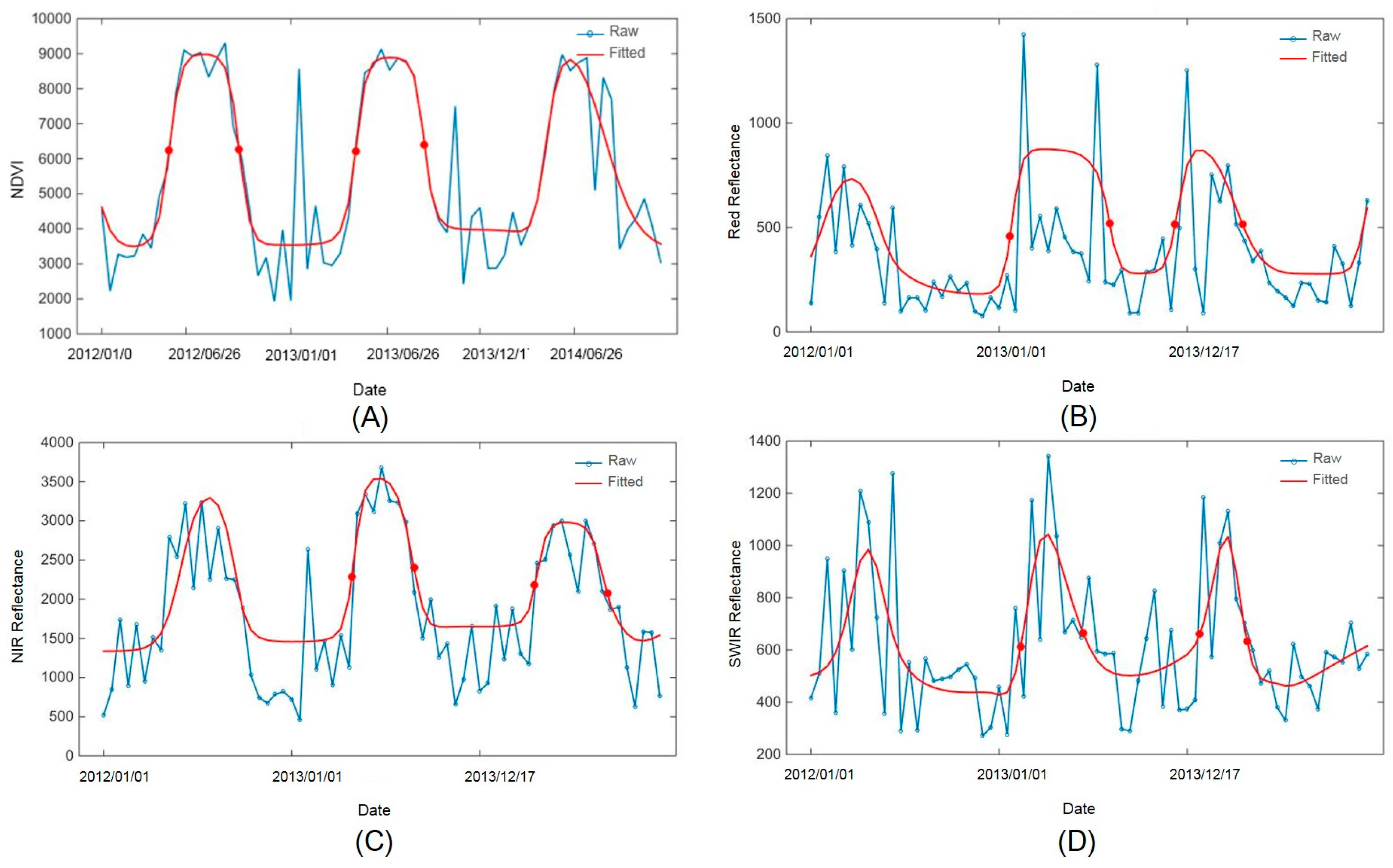
Figure 2 shows an example fit to NDVI, red, NIR, and SWIR temporally smoothed from a forest sample. The twelve phenological variables extracted for each growing season included: length of the season, base level (average of the left and right minimum values), largest data value for the fitted function during the season, seasonal amplitude, rate of increase at the beginning of the season, rate of decrease at the end of the season, small seasonal integral, large seasonal integral, number of seasons in a calendar year, time of the start of the season, time of the end of the season, and time of the middle of the season. Use of these temporal factors allowed the program to have ample data to fit a full function to the growing seasons of North Korea.

3.2. Reference Data Collection

3.2.1. Training Samples Collection

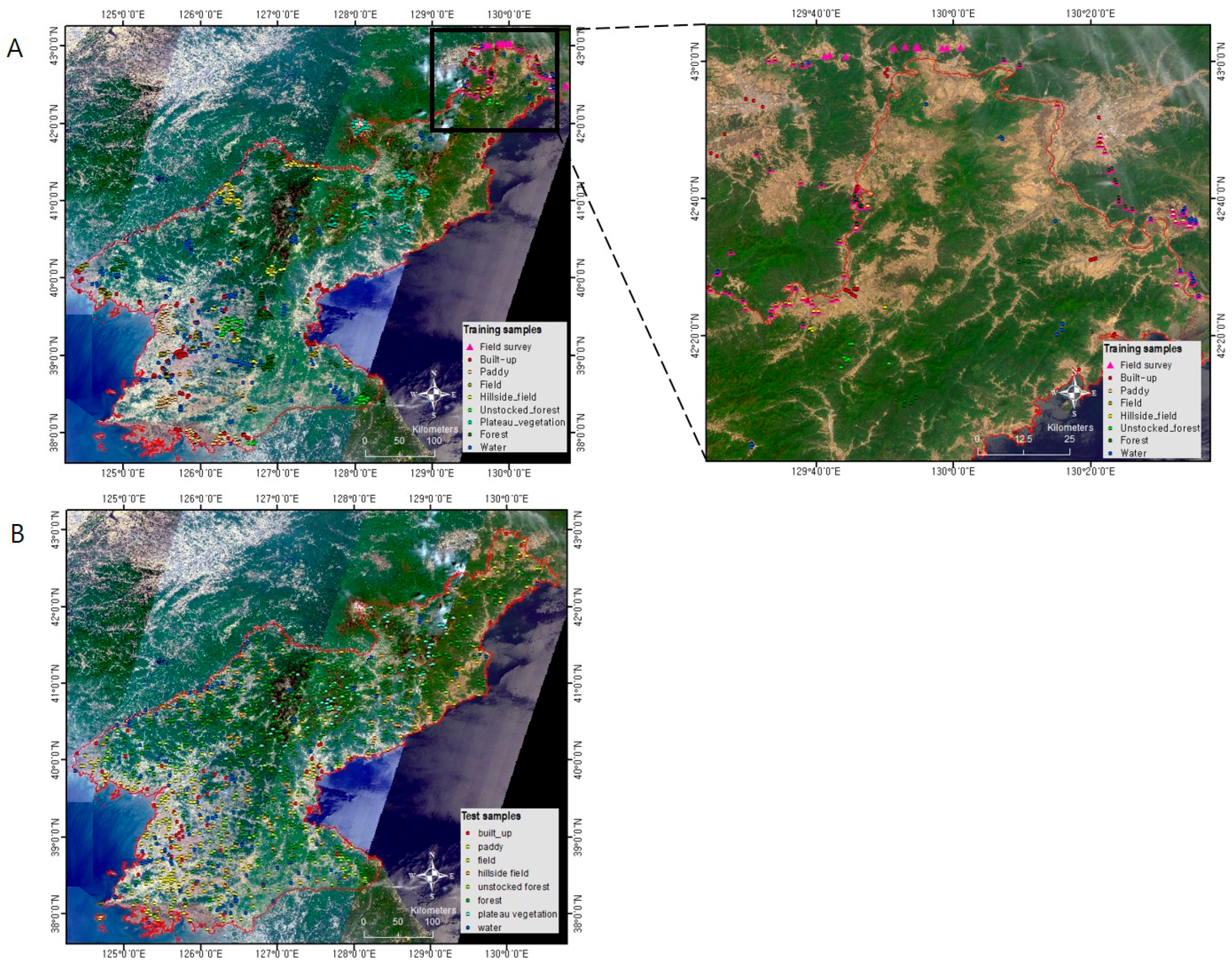
The representative samples for each class were collected by field survey, reference data from Google Earth and land cover map of North Korea which was provided by the Korean Forest Services in 2007. The direct collection of regions of interest (ROI) in the data-scarce, remote areas of North Korea is limited due to political conditions. In this study, we could only obtain field survey points from the China side of the North Korea-China border (Figure 3A). On the northern border along the Tumen River we were able to collect 112 GPS points and simultaneously observe the land cover types on the North Korean side of the river. We also interpreted the visual criteria of each land cover class (Table 1) in the satellite imagery of Quickbird and Google Earth [38]. Since GE launched in 2005, many studies have been conducted using GE to explore the reference data [15,39]. The hillside field and unstocked forest still have confusing visual characteristics in satellite images. Therefore, the land cover map of North Korea, classified using spot images, was referenced to distinguish deforestation types.
This sampling method was demonstrated to have high accuracy for use with RF [40]. All training points were selected across North Korea with point centers at least 500 m apart [15]. The land cover types of random points were identified by visual interpretation of each class (Table 1). The sample size per class was set to a minimum of 200 points for classification [41], and the total sample size was 1660 points containing the survey points (Figure 3).

3.2.2. Test Samples Collection

Ground truth points used for assessing the accuracy of our results were developed using a random sampling method, which helps ensure that test samples are chosen in an unbiased manner and in proportion to the underlying, but as yet unmapped, land cover-land use categories [42].
The random points made in ArcGIS 10.1 were overlaid on the Google Earth images identifying land cover classes by the visual criteria described in Table 1. The random samples of natural forest were overabundant; in contrast, there were few samples for built-up, paddy, plateau vegetation, and water, as these areas covered only small fractions of the landscape. Thus, we implemented a stratified random sampling [15] for these classes. The polygons for built-up, paddy, and water categories were extracted from the land cover map provided by the Korean Forest Service as reference, and the random points for these landscape were made. Since there was no information about the plateau vegetation on the forest map, random points for plateau vegetation were made within the polygons with elevation >1800 m. Finally, 999 sample points, with a minimum of 50 points in each class were selected based on the recommendations of Congalton and Green [42] at intervals over 500 m.

3.3. Normalized Indices

Normalized indices show a much higher classification accuracy compared with original un-transformed spectral data. This is because normalization can be used to compensate for changing conditions of illumination, surface slope, and spectral variability due to reduction of the viewing angle [43]. Such indices can effectively detect changes from early spring growth to late season maturity and senescence. In this study, we used multi-indices to enhance the classification accuracy with NDVI, NDSI, and NDWI, which indicated the existence of vegetation, soil, and water respectively [44]. The equations of the indices are as follows:
NDVI = NIR RED NIR + RED
NDSI = SWIR NIR SWI   R + NIR
NDWI = SWIR RED SWIR + RED
where red, NIR and SWIR are the surface reflectance for band 1, 2, and 7, respectively, of MODIS.
The NDVI is often used as an indicator to extract the seasonal data from the relationships between the spectral reflectance and vegetation canopy characteristics [45,46,47]. In this case, R-band was used to represent spectral absorption by vegetation and the NIR-band to represent the reflectance value (Equation (1)). Therefore, NDVI can characterize the properties of vegetation well [48,49]. NDVI is commonly used to make spatial and temporal comparisons of terrestrial photosynthetic activity; thus, it is one of the indicators of the state of land degradation and of the speed of increase or decrease of photosynthesis, which provides biophysical information [50,51,52].
The NDSI is more sensitive to canopy structure [53] because it identifies areas where soil is the dominant background or foreground material. NDSI uses the SWIR and NIR-bands (Equation (2)), where SWIR represents the difference in reflectance values between soil areas [54]. Thus, NDSI is a good indicator for separating areas of vegetation from areas of soil.
The NDWI, using NIR and SWIR reflectance values [55] (Equation (3)), is proposed for use in remote sensing of the liquid water content of vegetation canopies. It reflects surface canopy moisture and forest humidity [55,56]. The NDWI has been used for monitoring water stress [57], and for mapping burnt areas in boreal forest [58]. Thus, the changing pattern of the NDWI with the seasons could distinguish areas of natural vegetation, farmland, and soil, in relation to moisture.

3.4. Classification Algorithm Using RF and Validation

Random forest was used for classifying the deforested areas in this study. RF is an ensemble of classification trees intended to improve classification accuracy [59]. RF randomly selects samples of variables many times to produce a large number of classification trees. Each tree is individually trained on a bootstrapped sample of the training data and contributes a single vote for assignment of the most frequent class to the input data [59]. RF can handle thousands of input features, and has been applied recently in remote sensing studies [60,61,62].
Multi-temporal satellite images are effective for reducing the uncertainty associated with land cover change [63]. The traditional classification algorithms (such as maximum likelihood) may not be appropriate for the classification of combined multi-date images because of the heterogeneous spectral signature of land-cover categories over large areas. To overcome this problem, roles for the RF classifier have recently emerged in remote sensing, and RF has been applied successfully for classifying complex land-cover status and dynamics.
The RF was built using the software R 3.4.2 [64] and the random forest package [65]. The number of trees (ntree) was set to 500, which proved to be a sufficient number in previous experiments [62]. At each node, a number of variables (mtry) were randomly sampled from a random subset of the features, and 100 runs were performed. To estimate the accuracy of trees, the out-of-bag prediction was used to estimate the accuracy of all trees, which represents an unbiased estimate of map accuracy, as long as the reference data were obtained via probability sampling [18]. To verify the classification result, we used the confusion matrix to estimate overall, user’s and producer’s accuracies, and the kappa coefficient [66,67].

4. Results and Discussion

4.1. Temporal Indices of Land Cover Classes

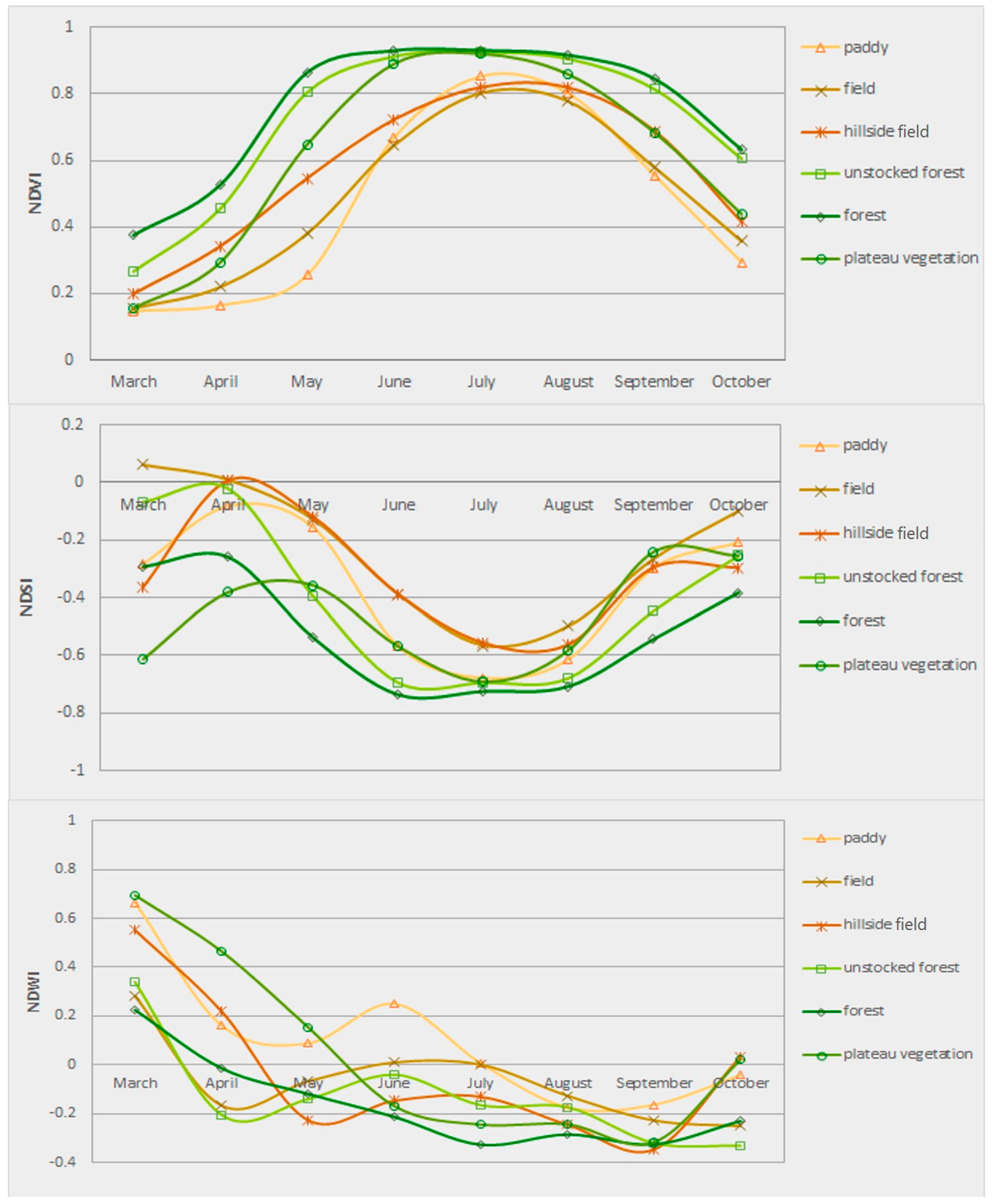
Figure 4 shows that the phenological characteristics (via NDVI, NDSI, and NDWI) of the paddies, flatland fields, hillside field, unstocked forest, forest, and plateau vegetation fluctuated during the growing season. The NDVI consistently increased from March to June for forest, unstocked forest, and plateau vegetation during the growing season, and decreased during the period from August to October (end of the growing season). For paddy, field, and hillside field the growing season extended to July. The highest NDVI value of all land cover classes was observed in July and August. All landscapes showed slightly different trends of change in NDVI value. Natural forest had the highest NDVI value during all periods (mainly consisting of trees) while unstocked forest consisting of grasses and shrubs had slightly lower NDVI values, but the curves followed the same general form. In the hillside fields, the crops were planted more densely than in the flat fields [56] with resultant NDVI values higher overall in comparison to flatland fields. Natural forest showed the highest NDVI value, followed by unstocked forest, plateau vegetation, and hillside fields, followed by the flatland fields and paddies.
NDSI decreased from April to June or July, depending on the landscape type, as the NDVI increased. Hillside fields exhibited the highest NDSI value among the forest landscapes when farmers were preparing the fields early in the season creating conditions for maximum soil exposure. In March–May, at the start of the growing season, the area of soil exposure in the four types of forest landscapes varied because of the canopy. In this case, the hillside fields had the highest NDSI values, followed by unstocked forest and forest. The highest NDWI value was observed at the start of the growing season because of snow melt when the canopy water content was at maximum.
When looking at the three individual graphs in Figure 4 one notices that the six landscape types followed similar trends by Index. However, the relative ranking of these landscape types varied according to the index being considered. The largest differences between forest landscape types occurred in different seasons based on the characteristics of each class. For example, hillside field and forest landscape types had similar trends of NDVI in the growing season and at the end of season. In these periods hillside fields had lower NDVI values of around 0.2, but in the middle of the season the difference narrowed to about 0.1 between hillside field and forest landscape types. It is important to note that the NDWI of plateau vegetation is higher than other classes because of the snow melt rate on plateaus was initially slower than for other forest landscape types, and this remained true until May. Additionally, the NDWI of paddies reached the summer maximum in June because of irrigation.

4.2. Temporal Indices of Land Cover Classes and Relevant Variables in the RF Classification

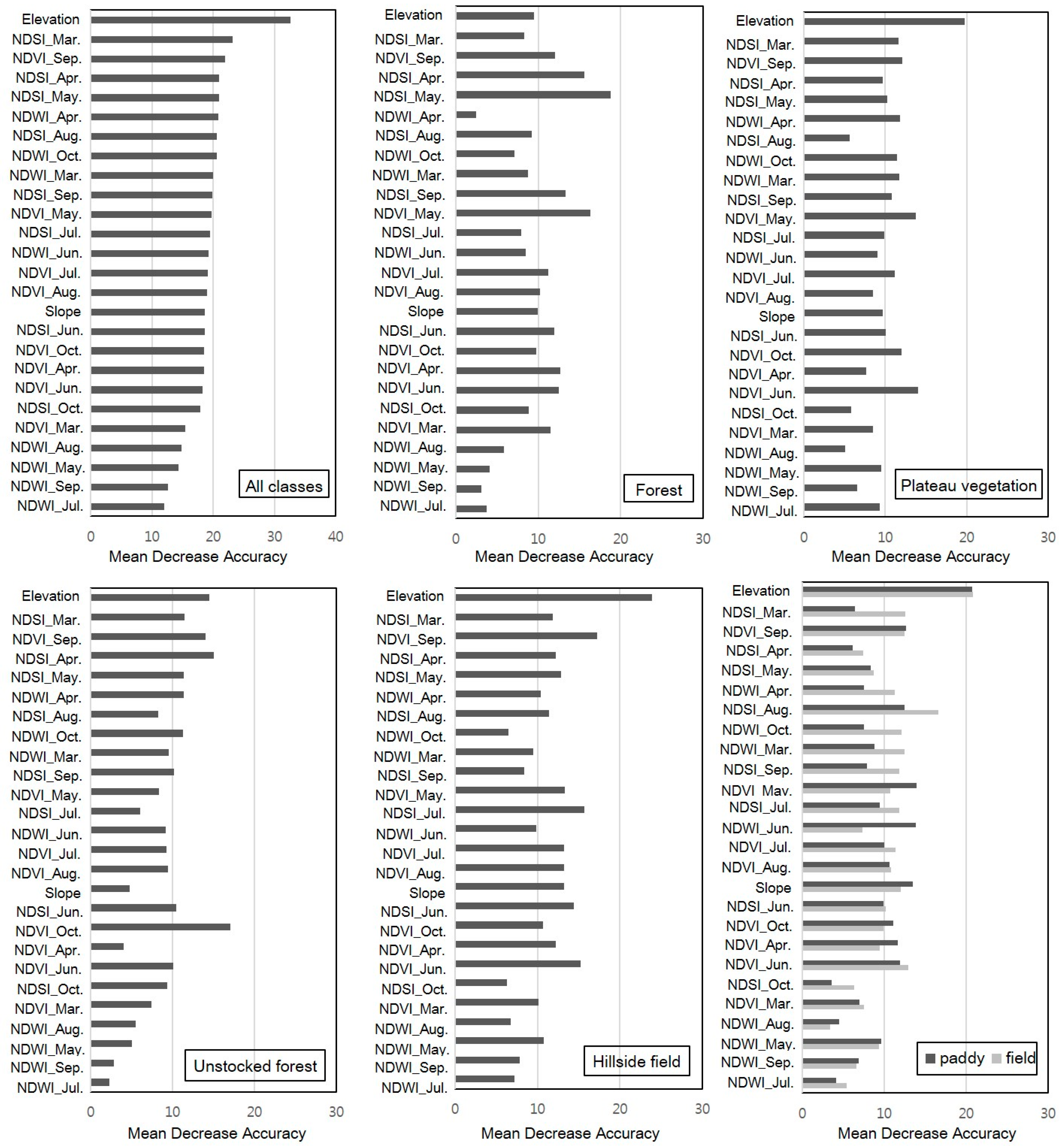
Using models with 500 trees, the importance of the contribution of each variable to the general classification model was calculated [59]. The mean decrease in accuracy displayed in Figure 5 is the contribution of each variable to the classification model generated by considering the seasonal multi-indices and topographic variables. Variables that have high mean decrease accuracy values are considered to be more important for overall or class-level classification [15].
According to the mean decrease in accuracy, the relevant variables in the RF classification were elevation, NDSI during the growing season (March–May), NDVI in September, and NDWI in April. In general, elevation contributed significantly to increased classification accuracy for each category (Table 2). Since the plateau vegetation, hillside field, and (flatland) field categories had similar NDVI patterns, but different topography, the priority variable for classifying these vegetation types was elevation. NDSI had a high value for exposed soils, and showed a large difference between vegetation types in March. Since field preparation for crops began in March [68], the fields became bare soil and presented the highest NDSI values while the other land-cover types were covered with vegetation or snow at the start of the season. Therefore, in March, NDSI could effectively distinguish (flatland) fields from other vegetation types. At the end of the growing season (September), differences in NDVI values could be observed between farmland (field and paddy) and forest (forest and unstocked forest). The forests were covered with vegetation while farmland (field and paddy) were ready to harvest. The NDWI value in April contributed to a classification for plateau vegetation. In the plateau area, the rate of snow melt was slower than other landscape types and the NDWI value at the start of the growing season was higher than for the other types. For this reason, this high value clearly distinguished the plateau sites from the other vegetation types that occurred near them.
The other variables in each season also contributed to increased accuracy in the classification of each vegetation type. The contributions of these variables are specific for North Korea. For mapping regions where there is heterogeneous vegetation cover, it is necessary to find the variables most effective for classification. Each vegetation type in each season, was representative of different vegetation, soil, and water conditions [44], so the phenology-based indices were found effective for classifying these vegetation cover types [15,18,69,70].

4.3. Classification Result and Accuracy Assessment

Classification results in this study demonstrated that phenology-based indices using RF classification are effective in mapping deforested land and in understanding complex vegetation cover. High classification accuracies were achieved (Table 2), and it was possible to successfully distinguish areas covered by shrubs, crops, and plateau vegetation which, in turn, distinguished unstocked forest, hillside field, and plateaus from forest. The producer’s accuracy in mapping the hillside field and unstocked forest was 80.3% and 87%, respectively, which indicates deforested areas. The corresponding user’s accuracies were 94% and 91.2%. Consequently, the overall accuracy of the resultant map was 89.38%, with a kappa coefficient 0.87 (Table 2). Since the landscape types within forests have similar variation in spectral signatures [71], hillside field was misclassified as other classes, such as flatland field or unstocked forest. Some areas of water were misclassified as built-up for the reason that the sand on the riverside was recognized as bare soil. This is a limitation of classification using data with 250 m resolution. This is a common problem when classifying heterogeneous landscapes using per-pixel classification techniques [72,73,74].
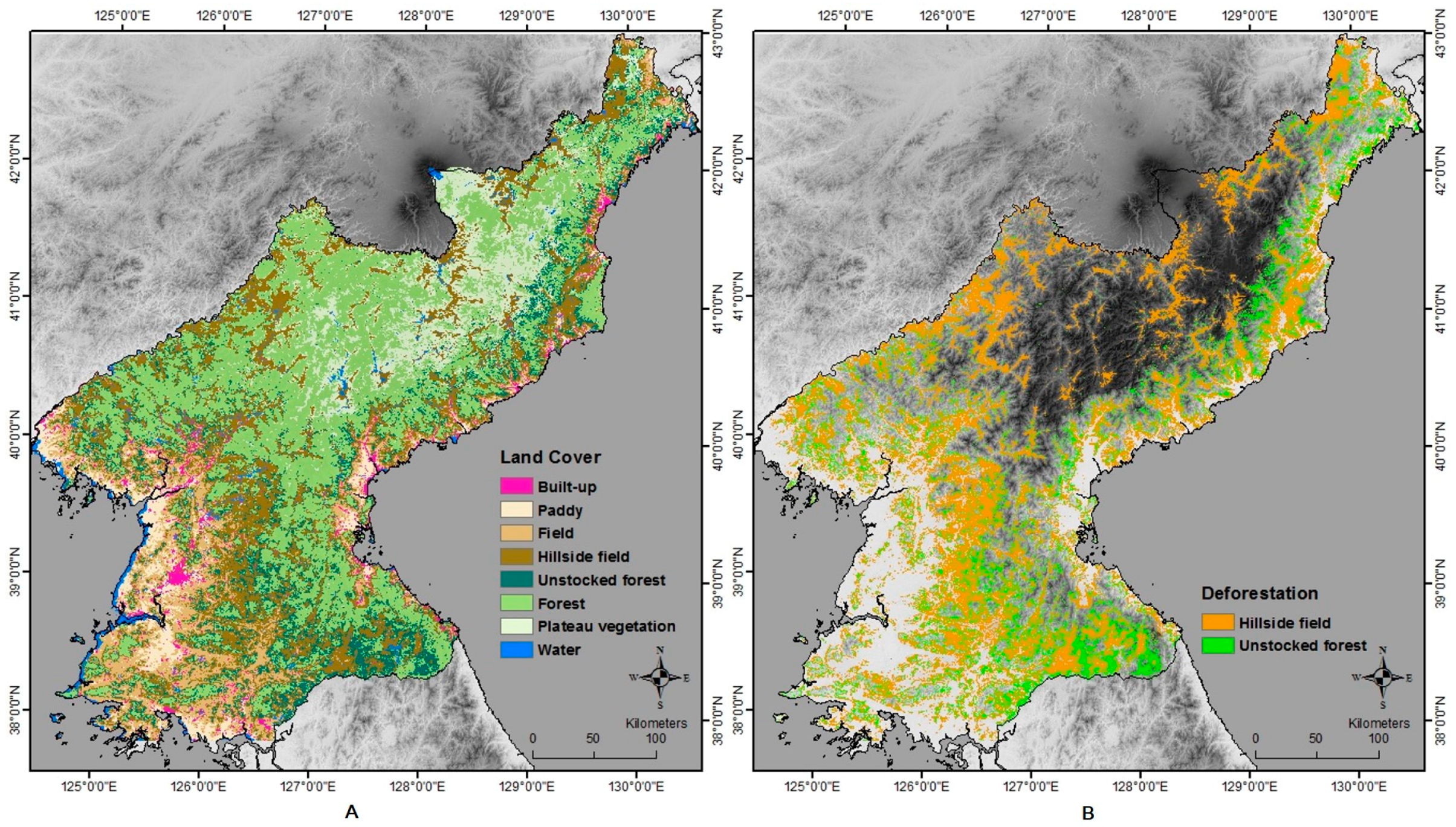
Figure 6A is the final classification map of the vegetation cover in North Korea, and Figure 5B shows the areas of deforestation in North Korea projected in this study. Approximately 4 million ha of forestland appeared deforested representing 34.2% of the total forestland in North Korea. In these areas forest was converted to hillside field (~2.7 million ha) and unstocked forest (~1.3 million ha) as shown in Figure 6B. Similar results were reported by Jeong [75] who also observed that about 30% of the forest was degraded in North Korea.
In North Korea, attempts to separate these cover types using traditional multispectral data or vegetation indices (Landsat, MODIS, or NDVI in one-time images) [9,75] have not been successful. The class accuracies indicated that phenology-based indices that also include vegetation, soil, and water information, along with the use of RF consistently increased the individual classification accuracies. Nevertheless, further research is needed to develop a technique to analyze detailed vegetation cover types at high spatial resolution.

5. Conclusions

The purpose of this study was to classify types of deforested areas caused by crop cultivation and logging and to increase the accuracy of classification over previous studies. We investigated a way to combine phenology-based multi-index distinctions derived from MODIS products and RF, as well as ways to distinguish complex, heterogeneous land cover in forests, such as hillside fields and unstocked forest, from plateau vegetation and natural forest. The outcomes of this study extend beyond those of most previous studies, which have usually been focused only on dryland forest. Previous work also involved the use of single image classifications based only on spectral data to distinguish the types of deforestation, and consequently had difficulty capturing the heterogeneous spectral signature of land cover categories over large areas. The outcomes of this study can be summarized as follows. First, the seasonal patterns indicated by three indices (NDVI, NDSI, and NDWI) showed differences typical of each type of vegetation cover in forest land, so it was possible to overcome the reflectance value confusion that occurs when using only one image, and to increase the classification accuracy. Second, to classify complex land cover and dynamics, RF proved itself a useful tool for classifying a variety of input features. Finally, the results highlighted the types of deforested land and their distribution in North Korea. That classification result showed overall accuracy of 89.38% when phenology-based multi-indices were combined with random forest. Our method greatly improved the classification accuracies for classification of heterogeneous vegetation cover and presented deforested areas more reliably. Therefore, it should be useful to continue monitoring variation of forest areas during forest restoration efforts in North Korea. The ecological impacts of forest degradation in the study area should also be urgently considered.

Acknowledgments

This work was supported by the BK21 Plus Project in 2016 (Seoul National University Interdisciplinary Program in Landscape Architecture, Global Leadership Program toward Innovative Green Infrastructure), Korea’s Ministry of Environment (Project No. 2014001310010) and Forest Science & Technology Projects (Project No. S111415L050100). The authors would like to thank the editor and anonymous reviewers for providing valuable suggestions to improve the quality of manuscript.

Author Contributions

Seunggyu Jeong designed the experiment and wrote the paper. Yihua Jin performed the data processing, analyzed the data and wrote the paper. Sunyong Sung contributed to random forest programming. Dong Kun Lee discussed the results and edited the manuscript. Gregory S. Biging helped interpret the results and did additional editing.

Conflicts of Interest

The authors declare no conflict of interest.

References

  1. Millennium Ecosystem Assessment (MEA). Ecosystems and Human Well-Being: Scenarios; Millennium Ecosystem Assessment: Washington, DC, USA, 2005. [Google Scholar]
  2. Abood, S.A.; Lee, J.S.H.; Burivalova, Z.; Garcia-Ulloa, J.; Koh, L.P. Relative contributions of the logging, fiber, oil palm, and mining industries to forest loss in Indonesia. Conserv. Lett. 2015, 8, 58–67. [Google Scholar] [CrossRef]
  3. Sasaki, N.; Putz, F.E. Critical need for new definitions of “forest” and “forest degradation” in global climate change agreements. Conserv. Lett. 2009, 2, 226–232. [Google Scholar] [CrossRef]
  4. Zheng, D.; Wallin, O.D.; Hao, Z. Rates and patterns of landscape change between 1972 and 1988 in the Changbai Mountain area of China and North Korea. Landsc. Ecol. 1997, 12, 241–254. [Google Scholar] [CrossRef]
  5. Bhatia, R.; Thorne-Lyman, A.L. Food shortages and nutrition in North Korea. Lancet 2002, 360, s27–s28. [Google Scholar] [CrossRef]
  6. Tang, L.; Shao, G.; Piao, Z.; Dai, L.; Jenkins, M.A.; Wang, S.; Wu, G.; Wu, J.; Zhao, J. Forest degradation deepens around and within protected areas in East Asia. Biol. Conserv. 2010, 143, 1295–1298. [Google Scholar] [CrossRef]
  7. Chazdon, R.L. Beyond deforestation: Restoring forests and ecosystem services on degraded lands. Science 2008, 320, 1458–1460. [Google Scholar] [CrossRef] [PubMed]
  8. Wilson, E.H.; Sader, S.A. Detection of forest harvest type using multiple dates of Landsat TM imagery. Remote Sens. Environ. 2002, 80, 385–396. [Google Scholar] [CrossRef]
  9. Cha, S.; Park, C.H. The utilization of google earth images as reference data for the multitemporal land cover classification with MODIS data of North Korea. Korean J. Remote Sens. 2007, 23, 483–491. [Google Scholar]
  10. Gómez, C.; White, J.C.; Wulder, M.A. Optical remotely sensed time series data for land cover classification: A review. ISPRS J. Photogramm. Remote Sens. 2016, 116, 55–72. [Google Scholar] [CrossRef]
  11. Souza, J.C.; Siqueira, J.; Sales, M.; Fonseca, A.; Ribeiro, J.; Numata, I.; Cochrane, M.; Barber, C.; Roberts, D.; Barlow, J. Ten-year landsat classification of deforestation and forest degradation in the Brazilian Amazon. Remote Sens. 2013, 5, 5493–5513. [Google Scholar] [CrossRef]
  12. Adam, E.; Mutanga, O.; Odindi, J.; Abdel-Rahman, E.M. Land-use/cover classification in a heterogeneous coastal landscape using rapideye imagery: Evaluating the performance of random forest and support vector machines classifiers. Int. J. Remote Sens. 2014, 35, 3440–3458. [Google Scholar] [CrossRef]
  13. Grimm, R.; Behrens, T.; Märker, M.; Elsenbeer, H. Soil organic carbon concentrations and stocks on barro colorado island—Digital soil mapping using random forests analysis. Geoderma 2008, 146, 102–113. [Google Scholar] [CrossRef]
  14. Baccini, A.; Goetz, S.J.; Walker, W.S.; Laporte, N.T.; Sun, M.; Sulla-Menashe, D.; Hackler, J.; Beck, P.S.A.; Dubayah, R.; Friedl, M.A.; et al. Estimated carbon dioxide emissions from tropical deforestation improved by carbon-density maps. Nat. Clim. Chang. 2012, 2, 182–185. [Google Scholar] [CrossRef]
  15. Clark, M.L.; Aide, T.M.; Grau, H.R.; Riner, G. A scalable approach to mapping annual land cover at 250 m using MODIS time series data: A case study in the dry chaco ecoregion of South America. Remote Sens. Environ. 2010, 114, 2816–2832. [Google Scholar] [CrossRef]
  16. Clerici, N.; Weissteiner, C.J.; Gerard, F. Exploring the use of MODIS NDVI-based phenology indicators for classifying forest general habitat categories. Remote Sens. 2012, 4, 1781–1803. [Google Scholar] [CrossRef] [Green Version]
  17. Eisavi, V.; Homayouni, S.; Yazdi, A.M.; Alimohammadi, A. Land cover mapping based on random forest classification of multitemporal spectral and thermal images. Environ. Monit. Assess. 2015, 187, 291. [Google Scholar] [CrossRef] [PubMed]
  18. Senf, C.; Pflugmacher, D.; van der Linden, S.; Hostert, P. Mapping rubber plantations and natural forests in Xishuangbanna (Southwest China) using multi-spectral phenological metrics from MODIS time series. Remote Sens. 2013, 5, 2795–2812. [Google Scholar] [CrossRef]
  19. Gartzia, M.; Alados, C.L.; Pérez-Cabello, F.; Bueno, C.G. Improving the accuracy of vegetation classifications in mountainous areas. Mt. Res. Dev. 2013, 33, 63–74. [Google Scholar] [CrossRef]
  20. Franklin, S.E.; Connery, D.R.; Williams, J.A. Classification of alpine vegetation using Landsat thematic mapper SPOT HRV and DEM data. Can. J. Remote Sens. 1994, 20, 49–58. [Google Scholar]
  21. Dymond, C.C.; Mladenoff, D.J.; Radeloff, V.C. Phenological differences in tasseled cap indices improve deciduous forest classification. Remote Sens. Environ. 2002, 80, 460–472. [Google Scholar] [CrossRef]
  22. Cha, S.; Seo, D.; Park, C. Monitoring vegetation phenology using MODIS in Northern Plateau region, North Korea. Korean J. Remote Sens. 2009, 25, 399–409. [Google Scholar]
  23. Schoene, D.; Killmann, W.; Lüpke, H.v.; LoycheWilkie, M. Definitional Issues Related to Reducing Emissions from Deforestation in Developing Countries; Food and Agriculture Organization of the United Nations: Rome, Italy, 2007. [Google Scholar]
  24. Land-Cover and Land-Use Change Program (LCLUC). Deforestation in North Korea. Available online: http://lcluc.umd.edu/hotspot/deforestation-north-korea (accessed on 2 January 2016).
  25. Thompson, I.D.; Guariguata, M.R.; Okabe, K.; Bahamondez, C.; Nasi, R.; Heymell, V.; Sabogal, C. An operational framework for defining and monitoring forest degradation. Ecol. Soc. 2013, 18, 20. [Google Scholar] [CrossRef]
  26. USGS Earth Explorer. Available online: http://earthexplorer.usgs.gov/ (accessed on 2 February 2016).
  27. Jensen, J.R.; Cowen, D.C. Remote Sensing of Urban/Suburban Socio-Economic Attributes. In Proceedings Land Satellite Information in the Next Decade II; American Society for Photogrammetry & Remote Sensing: Bethesda, MD, USA, 1997. [Google Scholar]
  28. Yool, S.R.; Makaio, M.J.; Watts, J.M. Techniques for computer-assisted mapping of rangeland change. J. Range Manag. 1997, 50, 307–314. [Google Scholar] [CrossRef]
  29. Jönsson, P.; Eklundh, L. Timesat—A program for analyzing time-series of satellite sensor data. Comput. Geosci. 2004, 30, 833–845. [Google Scholar] [CrossRef]
  30. Eklundh, L.; Jönsson, P. Timesat 3.2 Software Manual; Lund and Malmö University: Lund, Sweden, 2015. [Google Scholar]
  31. Viovy, N.; Arino, O.; Belward, A.S. The best index slope extraction (BISE)—A method for reducing noise in NDVI time-series. Int. J. Remote Sens. 1992, 13, 1585–1590. [Google Scholar] [CrossRef]
  32. Gutman, G.G. Monitoring land ecosystems using the NOAA global vegetation index data set. Glob. Planet Chang. 1991, 90, 195–200. [Google Scholar] [CrossRef]
  33. Holben, B.N. Characteristics of maximum-value composite images from temporal AVHRR data. Int. J. Remote Sens. 1986, 7, 1417–1434. [Google Scholar] [CrossRef]
  34. Lloyd, D. A phenological classification of terrestrial vegetation cover using shortwave vegetation index imagery. Int. J. Remote Sens. 1990, 11, 2269–2279. [Google Scholar] [CrossRef]
  35. Reed, B.C.; Brown, J.F.; Vanderzee, D.; Loveland, T.R.; Merchant, J.W.; Ohlen, D.O. Measuring phenological variability from satellite imagery. J. Veg. Sci. 1994, 5, 703–714. [Google Scholar] [CrossRef]
  36. Sellers, P.J.; Tucker, C.J.; Collatz, G.J.; Los, S.O.; Justice, C.O.; Dazlich, D.A.; Randall, D.A. A global 1-degrees by 1-degrees NDVI data set for climate studies. 2. The generation of global fields of terrestrial biophysical parameters from the NDVI. Int. J. Remote Sens. 1995, 16, 1571. [Google Scholar]
  37. Jonsson, P.; Eklundh, L. Seasonality extraction by function fitting to time-series of satellite sensor data. IEEE Trans. Geosci. Remote 2002, 40, 1824–1832. [Google Scholar] [CrossRef]
  38. Google Earth. Available online: https://www.google.com/earth/ (accessed on 15 August 2015).
  39. Hu, Q.; Wu, W.; Xia, T.; Yu, Q.; Yang, P.; Li, Z.; Song, Q. Exploring the use of google earth imagery and object-based methods in land use/cover mapping. Remote Sens. 2013, 5, 6026–6042. [Google Scholar] [CrossRef]
  40. Ye, Y.; Wu, Q.; Huang, J.Z.; Ng, M.K.; Li, X. Stratified sampling for feature subspace selection in random forests for high dimensional data. Pattern Recognit. 2013, 46, 769–787. [Google Scholar] [CrossRef]
  41. Li, C.; Wang, J.; Wang, L.; Hu, L.; Gong, P. Comparison of classification algorithms and training sample sizes in urban land classification with landsat thematic mapper imagery. Remote Sens. 2014, 6, 964–983. [Google Scholar] [CrossRef]
  42. Congalton, R.G.; Green, K. Assessing the Accuracy of Remotely Sensed Data: Principles and Practices, 2nd ed.; CRC Press: Boca Raton, FL, USA, 2009. [Google Scholar]
  43. Simonetti, E.; Simonetti, D.; Preatoni, D. Phenology-Based Land Cover Classification Using Landsat 8 Time Series; European Commission Joint Research Center: Ispra, Italy, 2014. [Google Scholar]
  44. Takeuchi, W.; Yasuoka, Y. Development of normalized vegetation, soil and water indices derived from satellite remote sensing data. J. Jpn. Soc. Photogramm. Remote Sens. 2004, 43, 7–19. [Google Scholar] [CrossRef]
  45. White, M.A.; Nemani, R.R. Real-time monitoring and short-term forecasting of land surface phenology. Remote Sens. Environ. 2006, 104, 43–49. [Google Scholar] [CrossRef]
  46. Richard, Y.; Poccard, I. A statistical study of NDVI sensitivity to seasonal and interannual rainfall variations in Southern Africa. Int. J. Remote Sens. 1998, 19, 2907–2920. [Google Scholar] [CrossRef]
  47. Wang, Q.; Adiku, S.; Tenhunen, J.; Granier, A. On the relationship of NDVI with leaf area index in a deciduous forest site. Remote Sens. Environ. 2005, 94, 244–255. [Google Scholar] [CrossRef]
  48. Setiawan, Y.; Kustiyo, K.; Darmawan, A. A simple method for developing near real-time nationwide forest monitoring for Indonesia using MODIS near- and shortwave infrared bands. Remote Sens. Lett. 2016, 7, 318–327. [Google Scholar] [CrossRef]
  49. Huete, A.; Didan, K.; Miura, T.; Rodriguez, E.P.; Gao, X.; Ferreira, L.G. Overview of the radiometric and biophysical performance of the MODIS vegetation indices. Remote Sens. Environ. 2002, 83, 195–213. [Google Scholar] [CrossRef]
  50. Ceccato, P.; Flasse, S.; Tarantola, S.; Jacquemoud, S.; Grégoire, J.-M. Detecting vegetation leaf water content using reflectance in the optical domain. Remote Sens. Environ. 2001, 77, 22–33. [Google Scholar] [CrossRef]
  51. Tucker, C.J. Remote sensing of leaf water content in the near infrared. Remote Sens. Environ. 1980, 10, 23–32. [Google Scholar] [CrossRef]
  52. Prince, S.D.; Goward, S.N. Global primary production: A remote sensing approach. J. Biogeogr. 1995, 22, 815–835. [Google Scholar] [CrossRef]
  53. Deng, Y.; Wu, C.; Li, M.; Chen, R. Rndsi: A ratio normalized difference soil index for remote sensing of urban/suburban environments. Int. J. Appl. Earth Obs. Geoinf. 2015, 39, 40–48. [Google Scholar] [CrossRef]
  54. Wolf, A. Using Worldview 2 Vis-NIR MSI Imagery to Support Land Mapping and Feature Extraction Using Normalized Difference Index Ratios; Digital Globe: Longmont, CO, USA, 2010. [Google Scholar]
  55. Gao, B.-C. NDWI—A normalized difference water index for remote sensing of vegetation liquid water from space. Remote Sens. Environ. 1996, 58, 257–266. [Google Scholar] [CrossRef]
  56. Jiang, Y.; Wang, T.; de Bie, C.A.J.M.; Skidmore, A.K.; Liu, X.; Song, S.; Zhang, L.; Wang, J.; Shao, X. Satellite-derived vegetation indices contribute significantly to the prediction of epiphyllous liverworts. Ecol. Indic. 2014, 38, 72–80. [Google Scholar] [CrossRef]
  57. Fensholt, R.; Sandholt, I. Derivation of a shortwave infrared water stress index from MODIS near- and shortwave infrared data in a semiarid environment. Remote Sens. Environ. 2003, 87, 111–121. [Google Scholar] [CrossRef]
  58. Fraser, R.H.; Li, Z. Estimating fire-related parameters in boreal forest using SPOT vegetation. Remote Sens. Environ. 2002, 82, 95–110. [Google Scholar] [CrossRef]
  59. Breiman, L. Random forests. Mach. Learn. 2001, 45, 5–32. [Google Scholar] [CrossRef]
  60. Rodriguez-Galiano, V.F.; Ghimire, B.; Rogan, J.; Chica-Olmo, M.; Rigol-Sanchez, J.P. An assessment of the effectiveness of a random forest classifier for land-cover classification. ISPRS J. Photogramm. Remote Sens. 2012, 67, 93–104. [Google Scholar] [CrossRef]
  61. Pal, M. Random forest classifier for remote sensing classification. Int. J. Remote Sens. 2005, 26, 217–222. [Google Scholar] [CrossRef]
  62. Senf, C.; Hostert, P.; van der Linden, S. Using MODIS time series and random forests classification for mapping land use in South-East Asia. In Proceedings of the 2012 IEEE International Geoscience and Remote Sensing Symposium (IGARSS), Munich, Germany, 22–27 July 2012; pp. 6733–6736.
  63. Grinand, C.; Rakotomalala, F.; Gond, V.; Vaudry, R.; Bernoux, M.; Vieilledent, G. Estimating deforestation in tropical humid and dry forests in madagascar from 2000 to 2010 using multi-date landsat satellite images and the random forests classifier. Remote Sens. Environ. 2013, 139, 68–80. [Google Scholar] [CrossRef]
  64. R Core Team. R: A Language and Envirionment for Statistical Computing; R Foundation for Statistical Computing: Vienna, Austria, 2009. [Google Scholar]
  65. Liaw, A.; Winener, M. Classificatn and regression by randomforest. R News 2002, 2/3, 18–22. [Google Scholar]
  66. Jensen, J.R. Introductory Digital Image Processing: A Remote Sensing Perspective; Prentice Hall: Upper Saddle River, NJ, USA, 2005. [Google Scholar]
  67. Jeong, S.G.; Mo, Y.; Kim, H.G.; Park, C.H.; Lee, D.K. Mapping riparian habitat using a combination ofremote-sensing techniques. Int. J. Remote Sens. 2016, 37, 1069–1088. [Google Scholar] [CrossRef]
  68. Boo, K.; Kim, U.; Kim, J.; Kim, C.; Soo, I.; Park, G.; Park, G.; Park, S.; Sohn, H.; Yu, B.; et al. Agriculture in North Korea: The Real State and Development Direction, 1st ed.; SNU Press: Seoul, Korea, 2001. [Google Scholar]
  69. Pan, X.-Z.; Uchida, S.; Liang, Y.; Hirano, A.; Sun, B. Discriminating different landuse types by using multitemporal NDXI in a rice planting area. Int. J. Remote Sens. 2010, 31, 585–596. [Google Scholar] [CrossRef]
  70. Richardson, A.D.; O’Keefe, J. Phenological differences between understory and overstory. Phenol. Ecosyst. Process. 2009, 87–117. [Google Scholar] [CrossRef]
  71. Immitzer, M.; Atzberger, C.; Koukal, T. Tree species classification with random forest using very high spatial resolution 8-band Worldview-2 satellite data. Remote Sens. 2012, 4, 2661–2693. [Google Scholar] [CrossRef]
  72. Zhang, J.; Li, P.; Wang, J. Urban built-up area extraction from landsat TM/ETM+ images using spectral information and multivariate texture. Remote Sens. 2014, 6, 7339–7359. [Google Scholar] [CrossRef]
  73. Duro, D.C.; Franklin, S.E.; Dubé, M.G. A comparison of pixel-based and object-based image analysis with selected machine learning algorithms for the classification of agricultural landscapes using SPOT-5 HRG imagery. Remote Sens. Environ. 2012, 118, 259–272. [Google Scholar] [CrossRef]
  74. Lu, D.; Weng, Q. A survey of image classification methods and techniques for improving classification performance. Int. J. Remote Sens. 2007, 28, 823–870. [Google Scholar] [CrossRef]
  75. Jeong, S.G.; Park, J.; Park, C.H.; Lee, D.K. Terrace fields classification in North Korea using MODIS multi-temporal image data. J. Korea Soc. Environ. Restor. Technol. 2016, 19, 73–83. [Google Scholar] [CrossRef]
Figure 1. Study site.
Remotesensing 08 00997 g001
Figure 2. Raw and fitted MODIS NDVI (A); red reflectance (B); NIR reflectance (C); and SWIR reflectance (D). TIMESAT seasonality variables derived from the functions are numbered on the figure for the interval from January 2012 to December 2013.
Remotesensing 08 00997 g002
Figure 3. Independent training samples (1660 points) (A) were collected regarding eight land cover classes in North Korea with a field survey; the 999 test points (B) used for the classification accuracy assessment were selected by random sampling. The displayed images are Landsat 8 OLE products.
Remotesensing 08 00997 g003
Figure 4. Time series indices of MODIS NDVI, NDSI, and NDWI (derived from RED, NIR, and MIR reflectance) for paddy, field, hillside field, unstocked forest, forest, and plateau vegetation categories. Random samples of 100 points were individually extracted for each type.
Remotesensing 08 00997 g004
Figure 5. Mean decrease accuracy values of overall and for each class from the RF classification using phenology-based multi-index and topographic variables.
Remotesensing 08 00997 g005
Figure 6. Final forest classification map of North Korea: (A) land cover map in North Korea; and (B) distribution of deforested land in North Korea.
Remotesensing 08 00997 g006
Table 1. Classification types and visual interpretation used for identifying training samples in satellite images.
ClassDescription
Built upUrban and buildings.
WaterbodyLakes, reservoirs and rivers.
PaddyFlooded field used to cultivate rice.
FieldCrop field with annual crops on flatland. This can be distinguished from paddy or other landscapes by the characteristics of plow lines, rectilinear shapes.
Hillside fieldCrop field with annual crops on the hillside. It can be detected by 3D view in Google Earth that offers elevation information.
Unstocked forestThis class is covered with shrubs or grasses, where crown cover of trees has fallen to <20% because of slash and burn. This class can be confused with hillside field, but it can be detected by the texture and whether there are plow lines or not.
Natural forestTrees are the major components.
Plateau vegetationThis class is covered with shrubs or grasses. It can be detected by elevation information and the distribution information from advanced research.
Table 2. Confusion matrix for land cover classification of North Korea.
Built-upPaddyFieldHillside FieldUnstocked ForestForestPlateau VegetationWaterTotalUser’s
Built-up5104000025789.5%
Paddy079153000310079%
Field0190800009990.9%
Hillside field00094105010094%
Unstocked forest00079320010291.2%
Forest0000123296034794.8%
Plateau vegetation0000086917888.5%
Water151351408711675%
Total66811121171073438093999
Producer’s77.3%96.3%80.4%80.3%87%96%86.3%93.5%
OOB estimate of error rate: 4.47%. Accuracy: 89.38%. Kappa: 0.8701.