1. Introduction
In recent years, with the successful launch of a series of high-spectral, high-spatial and high-temporal resolution active and passive satellite sensors, the remote sensing communities have accumulated a large amount of invaluable and irreplaceable data for global monitoring [
1]. The latest statistics shows that the current number of on-orbit satellite is 216 around the world, among them, 52 belonging to the USA [
2,
3]. The total EOSDIS accumulated data archive volume has been reached to 12.1 petabytes (PBs) around the year 2015 [
4]. Up to November 2016, the archived data volume of China’s FY satellite center has been up to 3.8 PBs [
5], and the resources satellite center of China has archived 16,024,310 scenes, about 8 PBs remote sensing data [
6].
Thus, there is often more than one type of remote sensing data in one place at one time, due to this large volume of data. In other words, there is more than one type of data selection for producing a certain remote sensing product [
7]. Therefore, we should select the most suitable data source from the redundant observation data. For example, if a user wants to generate the 30-m NDVI in a certain place during a certain time range, and there are Landsat-TM/ETM+/OLI and HJ1A/B-CCD several types of data for selection, then it is better to select the most suitable data source. It’s worth mentioning that, here “the most suitable data source”, denotes the best data for reflecting physical parameters of the ground surface, such as the land vegetative cover index, water coverage index, land use degree index, and alteration degree. In addition, during the process of product generation, two other cases also should be considered: (1) due to the fact that no single remote sensor can cover such a large area at one time, there is often a lack of sufficient special data for a long-term series observation of a large area of Earth. We should have to select substitute data for the missing data, if the prepared data source cannot cover the needed space and time; (2) if the best data source exists but is of poor quality, we should select the second- or third-best data for replacement.
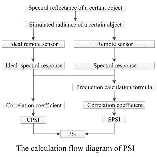
However, for the above-mentioned three cases, the current data selection strategy mainly adopts the empirical model, and has a lack of theoretical support and quantitative analysis. Therefore, we should explore a more scientific and reasonable data selection strategy. Based on the difference analysis of each remote sensor, this paper proposed a suitability evaluation model, providing guidance for data selection during the generation of remote sensing products. The model assumed an ideal remote sensor, which was with total reflection ability, as the evaluation standard. Based on the standard, the correlation coefficient of the spectral responses between a certain remote sensor and the ideal sensor would be calculated. The correlation coefficient stands for the comprehensive response ability of each remote sensor for a certain ground object, and it was named Comprehensive Production Suitability Index (CPSI). As for the specific remote sensing product, taking the spectral responses of the ideal and actual sensors’ bands into each product formula, the correlation coefficient of the formula calculations would be obtained, and named Specific Production Suitability Index (SPSI). Based on the CPSI and SPSI, the Production Suitability Index (PSI) would be obtained finally, and it will be taken as a reference for data selection.
In order to validate the proposed model, we chose two typical value-added information products, Normalized Difference Vegetation Index (NDVI) [
8] and Normalized Difference Water Index (NDWI) [
9], using Landsat-OLI and HJ1A-CCD1 image data, performed verification experiments. The suitability evaluation model would provide guidance for the most suitable data selection from redundant multisource remote sensing data, or selection of substitute data if data is lacking or poor quality, during the process of generating remote sensing products. Especially in the big data era [
10,
11,
12,
13], it would assist in the generation of standard, automated, serialized products, and play an important role in one-station, value-added information services.
The remainder of this paper is organized as follows:
Section 2 provides an overview of the background knowledge and related work;
Section 3 provides an overview of the suitability evaluation model;
Section 4 introduces the experiment and analysis of the proposed model;
Section 5 provides a summary and conclusions.
2. Background Knowledge and Related Work
The study object of the production suitability evaluation model is the remote sensing products. So, first, we must introduce the typical objects and their corresponding products. Related work is also addressed in this section.
2.1. Typical Objects and Corresponding Products
In general, the detection ability of the remote sensor depends on whether or not its spectral range covers the ground object’s character spectra. As for vegetation, its character spectra are the near-infrared-band and red-band spectra [
14]. The Landsat-TM/ETM+/OLI and HJ1A/B-CCD data, the spectral ranges of which cover the vegetation’s character spectra, may reflect the information of vegetation. As for the extraction of hydroxyl alteration information, because its character absorption spectra are located in the range of 2200–2500 nm, the Landsat-TM/ETM+/OLI and Aster data are the suitable sources [
15].
Furthermore, in order to realize the extraction of special information from the remote sensing images, scientists have built a series of typical remote sensing value-added data sets [
16] and their corresponding algorithms, such as NDVI, NDWI, Normalized Difference Drought Index (NDDI) [
17], Normalized Difference Build-up Index (NDBI) [
18], Normalized Difference Snow Index (NDSI) [
19], hydroxyl anomaly index [
20], silicide anomaly index [
21] and so on (
Table 1). These index products all reflect the situation of ground objects. For example, NDVI can reflect the growth and coverage situation of aboveground vegetation, as well as the biomass and vegetation types; NDWI shows the water coverage situation, and the hydroxyl or silicide anomaly indexes indicate the degree of rock alteration. This paper will use NDVI and NDWI as examples of two typical products; it then builds the suitability evaluation model and verifies it.
2.2. Related Work
The production suitability evaluation is the spectral response variance analysis of each remote sensor, essentially. And there are many studies examining the differences in interaction between remote sensors. For example, Steven et al. (2003) showed that when NDVI from the different instruments were compared, they varied by a few percent, but the values were strongly linearly related, allowing vegetation indices from one instrument to be intercalibrated against another. They also presented a table of conversion coefficents for AVHRR, ATSR-2, Landsat MSS, TM and ETM+, SPOT-2 and SPOT-4 HRV, IRS, IKONOS, SEAWIFS, MISR, MODIS, POLDER, Quickbird and MERIS [
22]. Goward et al. (2003) showed that the red band reflectance of IKONOS is higher than that of the ETM+, but the near-infrared band is opposite [
23]. Soudani et al. (2006) compared NDVI, SAVI and ARVI of ETM+, SPOT and IKONOS data respectively; the results showed that all of the vegetation indexes of ETM+ and SPOT are higher than those of IKONOS [
24]. Van Leeuwen et al. (2006) found that the NDVI data, which is inversed of the MODIS images, is higher than that of AVHRR [
25]. Martínez-Beltrán et al. (2009) compared and analysed NDVI data which was separately inversed from the ETM+, TM, IRS-LISS, Aster, QuickBird and ACHRR, and also established the conversion coefficient between each remote sensor [
26]. Song et al. (2010) validated a linear relationship between the NDVI values acquired from the VGT and AVHRR sensors, using an unbiased comparison between the two datasets [
27]. Fensholt and Proud (2012) evaluated the accuracy by comparison with the global Terra MODIS NDVI (MOD13C2 Collection 5) data using linear regression trend analysis, and found that the trends of GIMMS NDVI was in overall acceptable agreement with MODIS NDVI data [
28]. Li et al. (2014) compared vegetation indices derived from Landsat-7 Enhanced Thematic Mapper Plus (ETM+) and Landsat-8 Operational Land Imager (OLI) sensors, and found that vegetation indices indicated that both sensors had a very high linear correlation coefficient [
29]. By comparison with multiple satellite sensors and in-situ observations, Ke et al. (2015) found that Landsat 8 OLI produced higher spatial variability of NDVIs than Landsat 7 ETM+ at vegetated and urban areas, but lower variability on water area [
30].
However, these studies did not begin with the point of product generation; nor did they provide the PSI for the remote sensing data according to specific evaluation standards. In addition, as for the current data selection strategy during the process of generating remote sensing products, it mainly adopts the empirical model, lack of theoretical support and quantitative analysis. However, with the arrival of the big data era in Earth observation, standard, automated, serialized product generation has become a trend. Hence, we should build the production suitability index for each remote sensor, and automatically select the best data source during the process of generating remote sensing products, according to the indexes.
3. Suitability Evaluation Model
In evaluating suitability for product generation from multisource remote sensing data, building an evaluation standard is the first step [
31]. Here, we assumed an ideal remote sensor with total reflection ability as the evaluation standard. In addition, under the natural condition, the total radiance reaching the sensor is always impacted by atmosphere. Therefore, in this paper, first, we assumed the object’s standard spectral curve, which was from the USGS standard spectral library or other field measurement results, as the object reflective spectrum. Then, taking the standard spectral curve as input, compute the total radiance at the entrance aperture of the sensor, by the aid of the radiative transfer software MODTRAN (MODerate resolution atmospheric TRANsmission) [
32]. The MODTRAN configuration parameters are listed in
Table 2.
Then, the simulated total radiance reaching the sensor will be obtained. Its spectral responses with each sensor is the Digital Number (DN) value, that records the intensity of electromagnetic energy measured for the ground resolution cell represented by that pixel. Finally, based on the standard presented above, the correlation coefficient of the spectral responses between a certain remote sensor and the ideal sensor would be calculated. The correlation coefficient stands for the comprehensive response ability of each remote sensor for a certain ground object, and it was named CPSI. As for the specific remote sensing product, taking the spectral responses of the ideal and actual sensors’ bands into each product formula, the correlation coefficient of the formula calculations would be obtained, and named SPSI. In addition, the following needs to supplement the calculation: in general, calculating remote sensing products should use the surface reflectance values instead of DN values associated with a satellite image; but here, the SPSI calculation is based on the evaluation standard, and it is essentially a relative value. Hence, taking the DN value into each product formula is reasonable in this circumstances. Based on the CPSI and SPSI, the PSI would finally be obtained, and it will be taken as a reference for data selection. Below, we will detail the suitability index and suitability evaluation model building process.
3.1. Comprehensive Production Suitability Index
The suitability of value-added information produced from multisource remote sensing data depends mainly on the spectral response between the total radiance reaching the sensor and the spectral response function of the sensor. Assuming that under the same atmospheric transmission conditions and the same geometrical view conditions, the total radiance at the entrance aperture of each remote sensor is
(
λ is the wavelength), and the band k spectral response function of each sensor is
, with corresponding spectral range
. Then the band k normalized response
at the entrance aperture of each remote sensor is as follows [
33,
34].
where the length of the effective wavelength
is calculated as the following equation [
35].
stands for the length of the effective spectrum, and
is the minimum wavelength of band k, and
is the maximum. The relationship between
,
and
,
are as following.
In order to compare the spectral response of different remote sensors, we assumed a certain object’s radiance curve
, which is through the influence of atmosphere, as the spectral response at the entrance aperture of the remote sensor, i.e., assuming
, where A denotes the influence of atmosphere. The corresponding reflectance spectral curve of
is
, which was from the USGS standard spectral library or other field measurement results. Then the ground object’s normalized spectral response
of band k is as follows.
In the meantime, we assumed an ideal remote sensor as the reference standard, and its corresponding bands all have total reflection ability, i.e.,
where
denotes the band k spectral response function of the ideal sensor. Then the normalized spectral response
of the ideal remote sensor is as follows [
36].
The correlation coefficient of the normalized spectral response between a certain remote sensor (
) and the ideal sensor (
) stands for the response ability of the remote sensor. Here, the calculation of the correlation coefficient adopts Spectral Angle Mapper (SAM), which only measures differences in spectral shape [
37]. The correlation coefficient between
and
only considers the spectrum shape change due to the affect of remote sensor spectral response
, it is insensitive to differences in the albedo of the object’s standard spectrum
.
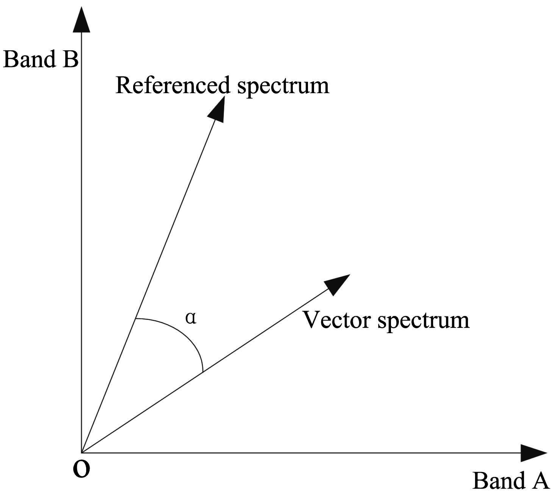
SAM is a similarity measuring method that is based on the similarity of the spectral curve. It matches the vector spectrum with the referenced spectrum from a k-dimensional perspective. The similar function is defined as the cosine of the generalized angle between the two vectors, which is the widely applicable generalized angle matching model. The spectral response of the k bands can be viewed as vectors in k-dimensional space. The degree to which it matches the spectrum unit will be calculated. The smaller the angle, the more similar they are [
38,
39] (
Figure 1).
The cosine of the generalized angle is as follows:
where
γ is the correlation coefficient between
and
, k is the band number, X and Y are the spectral responses of the two spectrum vectors,
α is the spectral angle.
The correlation coefficient of all character bands represents the entirety of the reflection and absorption characteristics; it also stands for the comprehensive representational ability of the sensor, called the CPSI. Regarding vegetation, the CPSI eliminates the influence of season and vegetation growth state; it is the measure of the sensor’s integrated radiation performance.
3.2. Specific Production Suitability Index
In addition, in order to calculate the suitability of a specific remote sensing product for each remote sensor, we also need to include
and
in each product formula P, and calculate the correlation coefficient of the two former results (
and
). Due to the result of each product formula is just only a figure, and it is not suitable for using SAM to calculate the correlation coefficient. Therefore, here, the correlation coefficient calculation just use the ratio method to compare the closeness degree of
and
. The correlation coefficient stands for the generation suitability of the specific remote sensing product, called the SPSI.
where
ρ is the correlation coefficient between
and
. For vegetation, the SPSI takes into consideration the influence of season, vegetation growth state, atmospheric conditions, solar zenith angle and other factors; it is the measurement of the remote sensor’s detection sensitivity.
3.3. Production Suitability Index
Based on the above CPSI and SPSI, we can get the PSI of a certain type of remote sensing product for each remote sensor, and its calculation model is as follows:
where
, i.e., if the spectral range
of the remote sensor covers the ground object’s character spectrum
,
, otherwise
.
4. Experiments and Discussion
In order to verify the correctness of the proposed model, we chose two typical products, NDVI and NDWI, as examples, and used Landsat-OLI and HJ1A-CCD1 images as the data sources to carry out verification experiments. NDVI and NDWI are two important parameters for describing the characteristics of land surface, and have been widely used in ground targets classification, ocean boundary information extraction, and other remote sensing applications. Especially, NDVI can be used as the major raw material for other complex vegetation products, such as Leaf Area Index (LAI), Photosynthetic Active Radiation (PAR), Net Primary Productivity (NPP) and so on. In addition, vegetation and water, as the main object type in the nature, generally have some standard spectral curves, which could be used as one of the references of the production suitability evaluation. Therefore, based on the standard spectral curves of vegetation and water, this paper chose NDVI and NDWI as examples of two typical products. Landsat-OLI and HJ1A-CCD1 images both have around 30 m spatial resolution, and both can be able to cover the visible and NIR (Near Infrared Spectrum) spectral range, as well as both have a strong detection ability for vegetation, water, ice, soil, et al. Landsat-OLI and HJ1A-CCD1 two types remote sensor, could be viewed as the typical examples of the similar or complementary remote sensors. Hence, we chose these two types of images as the experimental data sources.
4.1. Satellite Data Sources
4.1.1. Landsat-OLI
Landsat 8 is an American Earth observation satellite launched on 11 February 2013. It was deployed at an altitude of 705 km, and it took about 16 days to scan the entire earth. Landsat 8 carries two instruments, the Operational Land Imager (OLI) sensor and Thermal Infrared Sensor (TIRS). These sensors both provide improved signal-to-noise (SNR) radiometric performance quantized over a 12-bit dynamic range. Especially, Landsat-OLI collects data from nine spectral bands. Seven of the nine bands are consistent with the Thematic Mapper (TM) and Enhanced Thematic Mapper Plus (ETM+) sensors found on earlier Landsat satellites, providing for compatibility with the historical Landsat data, while also improving measurement capabilities. Two new spectral bands, a deep blue coastal/aerosol band and a shortwave-infrared cirrus band, will be collected, allowing scientists to measure water quality and improve detection of high, thin clouds [
29].
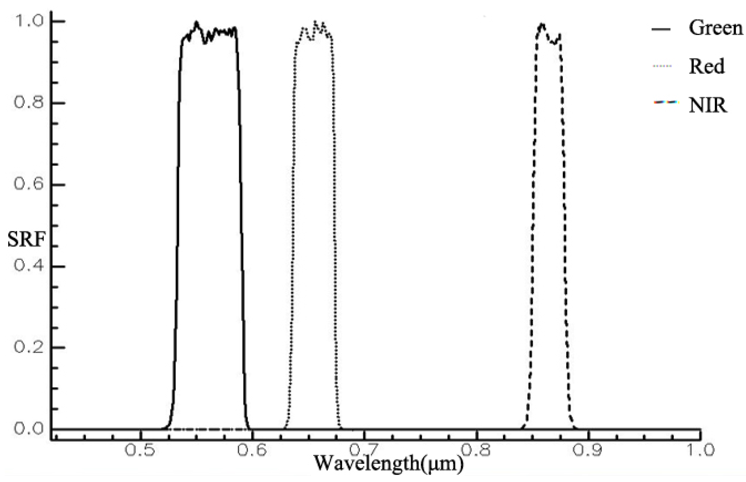
In order to establish NDVI and NDWI suitability evaluation models, the green, red and NIR bands of Landsat-OLI data should be considered. Their effective spectral ranges are 0.533–0.590
m, 0.636–0.673
m and 0.851–0.879
m [
30,
40]. After spectrum fitting and resampling, the continuous spectral response functions were obtained; see
Figure 2.
4.1.2. HJ1A-CCD1
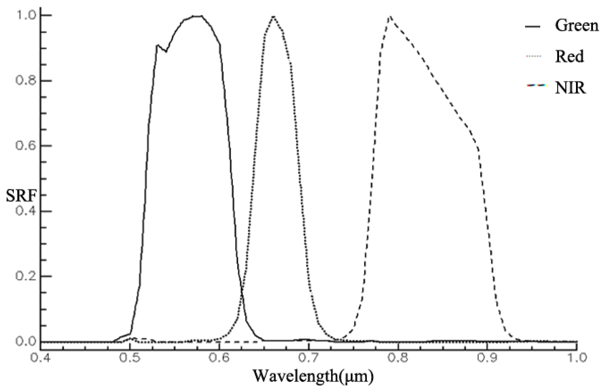
The HJ-1A satellite was the first in a series of environment and disaster monitoring satellites. It was launched in 2008. Its orbit altitude is 650 km, and the orbit inclination is 98 degrees. The HJ-1A satellite has two CCD sensors and an HSI sensor. The CCD sensor has an image swath of about 360 km, with blue, green, red, and NIR bands, 30m ground pixel resolution, and a 4-day revisit period. The effective spectral ranges are 0.52–0.60
m, 0.63–0.69
m and 0.76–0.90
m of green, red and NIR bands [
41,
42], and their fitted and resampled spectral functions are as shown in
Figure 3.
4.2. Suitability Evaluation Model of NDVI
4.2.1. Character Spectrum and Standard Spectral Curves of Vegetation
The obvious characteristics of healthy vegetation are the 10%∼20% small reflectance peaks near 0.55
m and two obvious absorption valleys near 0.45
m and 0.65
m. In the range of 0.7∼0.8
m, it is a steep slope and the reflectance increases sharply. In the 0.8∼1.3
m near-infrared band, there is a high or higher than 40% reflectance peak [
43,
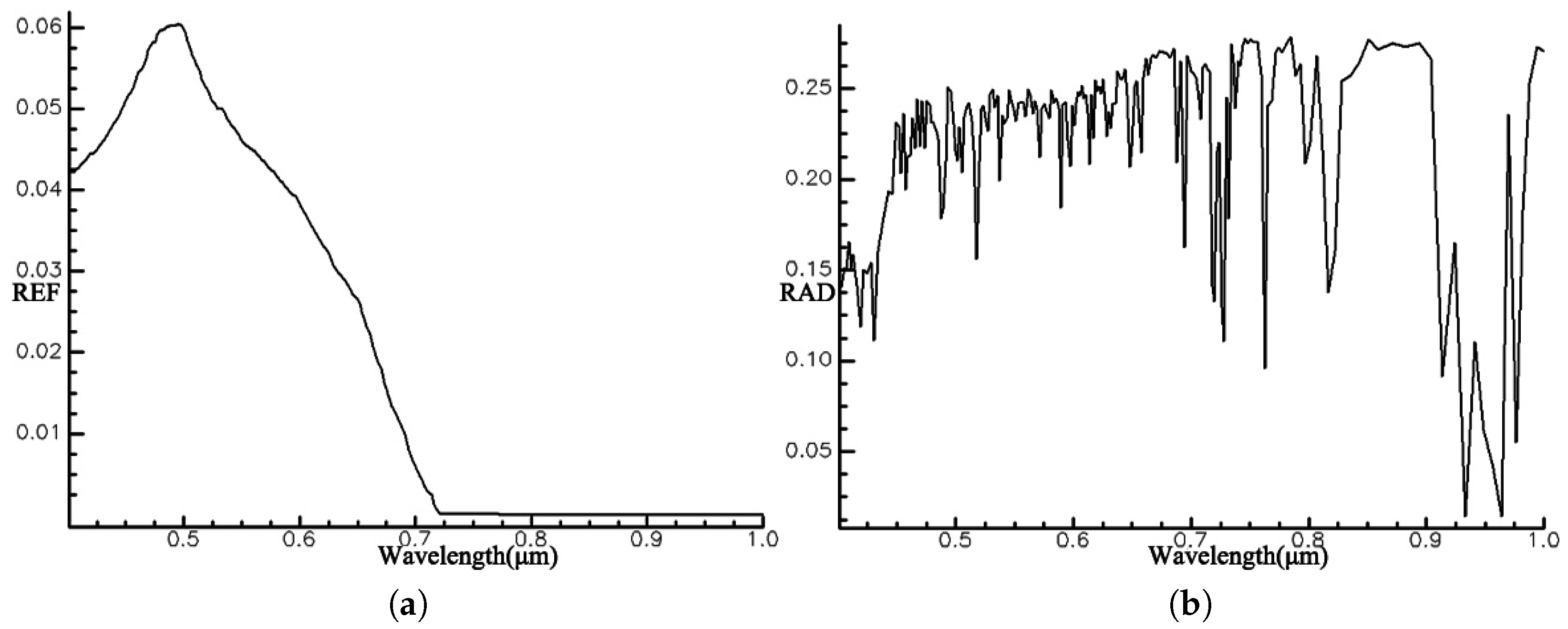
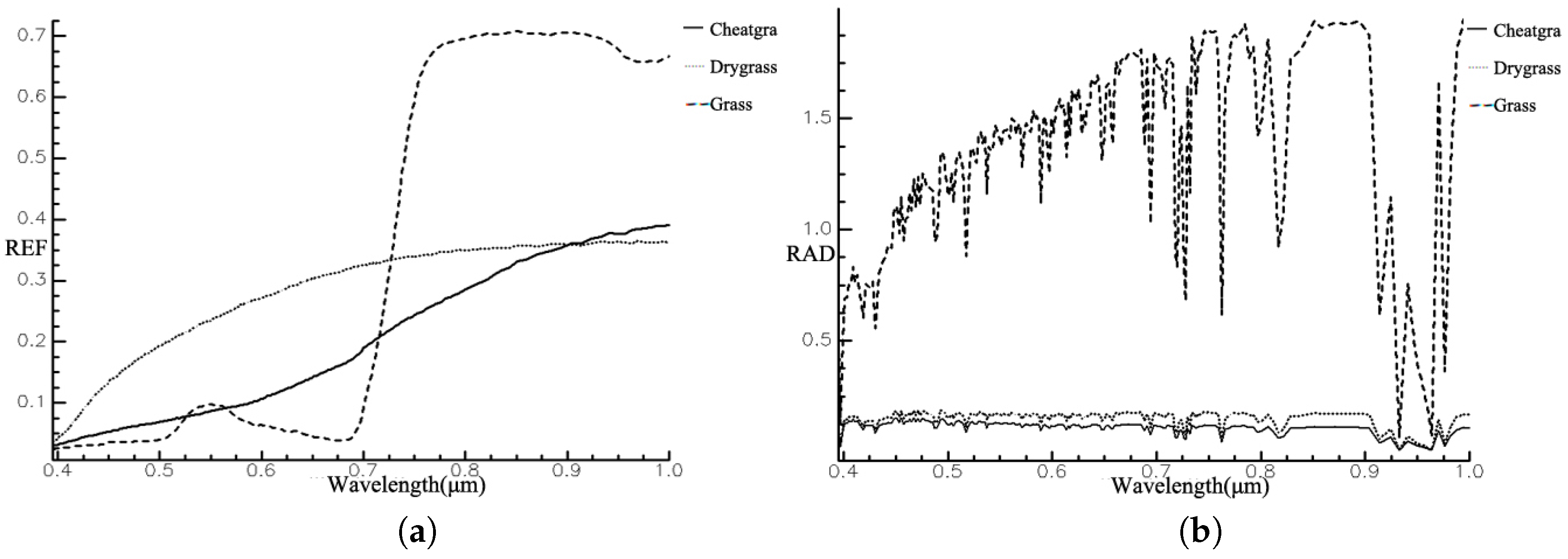
44]. Therefore, the highly absorbent red band and high-reflectivity near-infrared band would be selected to establish NDVI, which is typically used to indicate the amount, or relative density, of green vegetation present in an image. In the visible region, the vegetation spectral response is mainly dominated by chlorophyll, and also greatly affected by season variation. In order to accurately compare vegetation detection ability of different remote sensors, we chose Cheatgra.spc, Grass.spc and Drygrass.spc, three standard spectral curves as the referenced spectrum from the USGS standard spectral library, presenting the seedling, mature and ageing periods of vegetation respectively [
45,
46]. Their standard reflectance spectral curves are as shown in
Figure 4a, and corresponding simulated radiance reaching the sensor are as shown in
Figure 4b. Especially, the MODTRAN configuration parameters for radiance simulation are in accordance with
Table 2.
By resampling the above standard spectral curves according to the spectrum intervals of Landsat-OLI or HJ1A-CCD1 data, and interpolating using smoothing spline in MATLAB [
47], the final continuous spectrum curves
,
,
will be obtained.
4.2.2. NDVI PSI computing
The NDVI PSI computing includes CPSI, SPSI and PSI computation based on three standard spectral curves, the Cheatgra.spc, Grass.spc and Drygrass.spc, and below we will detail the three parts.
CPSI of NDVI
where
was set equal to
,
,
separately, and
,
,
, and
were set equal to the effective spectral ranges of red and NIR bands of Landsat-OLI and HJ1A-CCD1 sensors. Finally, the CPSI of Cheatgra.spc, Grass.spc and Drygrass.spc could be obtained as shown in
Table 3.
SPSI of NDVI
where
and
were set equal to the red and NIR bands’ normalized response function of Cheatgra.spc, Grass.spc and Drygrass.spc, and their corresponding SPSI were calculated as shown in
Table 4.
Based on the above results, the NDVI PSI of Cheatgra.spc, Grass.spc and Drygrass.spc can be obtained as shown in
Table 5.
As can be seen in
Table 5, no matter the growing season, the NDVI PSI of Landsat-OLI is higher than that of HJ1A-CCD1. In other words, the vegetation detection ability of Landsat-OLI is better than that of HJ1A-CCD1, and the Landsat-OLI data is more suitable for NDVI production than HJ1A-CCD1 data.
4.2.3. Results and Analysis
To test the validity of NDVI SPI, we selected Landsat-OLI (LC81220442013333LGN00.tar.gz) and HJ1A-CCD1 (HJ1A-CCD1-456-88-20131129-L20001092305.tar.gz) images separately, which were obtained in southern China, on 29 November 2013. As for OLI data, the atmospheric correction method we used was the FLAASH (Fast Line-of-sight Atmospheric Analysis of Spectral Hypercubes) algorithm [
48]. The atmospheric correction method of the HJ1A-CCD1 data is the relative radiation correction based on Pseudo Invariant Features (PIF) [
49], a reference to the radiation-corrected OLI data. The geometric correction method of the HJ1A-CCD1 data is the rational function model (RFM) [
50], with the OLI image for geo-reference [
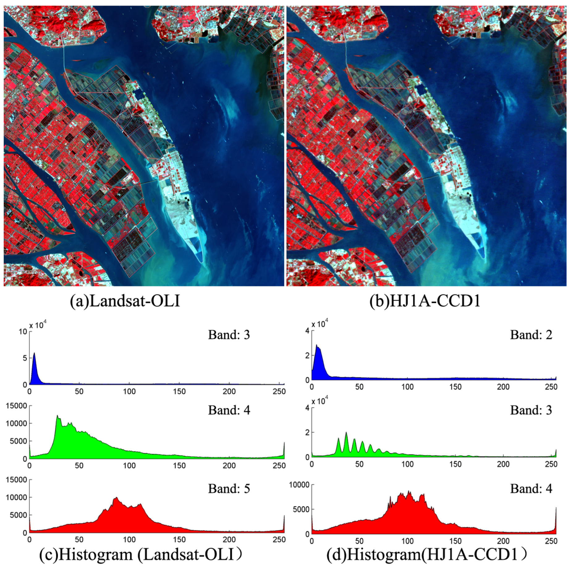
51]. After atmospheric correction and resizing, a subset of each image area (800 pixels × 800 pixels) was extracted in a region of vegetation cover zones. Their reflectance images are as shown in (
Figure 5a,b) (stretching gray scale range to 0–255 for display enhancements), and a corresponding histogram graph of each image was as shown in
Figure 5c,d.
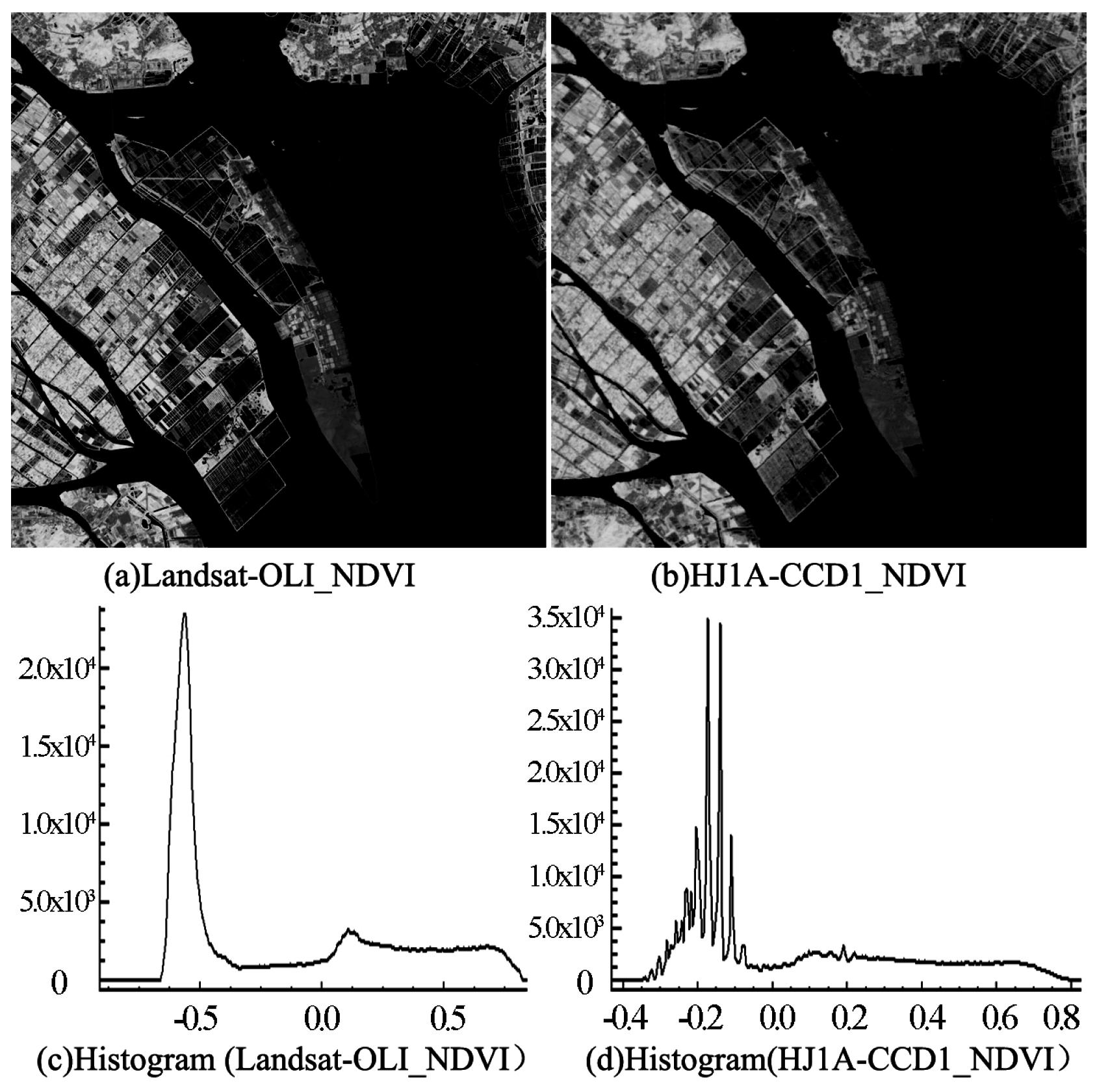
Then the NDVI of each image was calculated using the NDVI computational formula; the results are shown in
Figure 6a,b, and their corresponding histogram graphs are as shown in
Figure 6c,d. As can be seen in
Figure 6c,d, there are two obvious peaks in Landsat-OLI NDVI histogram, and no obvious peaks on zero right side appeared in HJ1A-CCD1 NDVI histogram, except for several pulse peaks around −0.2. For further detailed analyses, qualitative and quantitative interactive comparisons will be made.
The qualitative comparison depends mainly on visual inspection. Thresholds would be developed based on histogram graphs and observed vegetation characteristics in our test images. Results of the analysis indicate the following NDVI vegetation thresholds: low confidence (NDVI ≥ 0.2), medium confidence (NDVI ≥ 0.3), and high confidence (NDWI ≥ 0.45) (
Figure 7). In addition, in order to show the amount of vegetation information extracted from Landsat-OLI and HJ1A-CCD1 images, the pie chart of each threshold image was obtained, and “1” denotes vegetation information.
As shown in
Figure 7, under the same threshold, the total amount of vegetation information extracted from HJ1A-CCD1 NDVI image is larger than that of Landsat-OLI NDVI image in each threshold, but some roads, buildings and water borders were also misclassified as vegetation in HJ1A-CCD1 NDVI image. Especially with the increase of the segmentation threshold, some water borders information gradually reduced or even disappear in HJ1A-CCD1 NDVI image, but the water borders in Landsat-OLI NDVI image are still obvious. Therefore, preliminary conclusion is that the vegetation information extracted from Landsat-OLI NDVI image is more accurate than that of HJ1A-CCD1 NDVI image. In other words, the vegetation detection ability of Landsat-OLI is better than that of HJ1A-CCD1.
In addition, in order to quantitatively compare virtues or defect degree of the two NDVI images, the precision evaluation would be carried out for the NDVI threshold images using the same classified samples [
52,
53] (
Table 6). It is worth mentioning that, the classified samples mainly include two types: (1) vegetation samples, which were uniformly sampled from grassland, forest land, arable land and city green belt, a total of 2989 pixels; (2) non-vegetation samples, which were uniformly sampled from water, building, bare land and other non-vegetation areas, a total of 3011 pixels.
As shown in
Table 5, in each segmentation threshold, the vegetation user’s accuracy and overall classification accuracy of Landsat-OLI NDVI is higher than those of HJ1A-CCD1 NDVI, and this indicates that some vegetation information may be misclassified in HJ1A-CCD1 NDVI image relative to Landsat-OLI NDVI image. As we know, the user’s accuracy is a measure indicating the probability that a pixel is Class A given that the classifier has labelled the pixel as Class A, essentially quantifying the errors of commission [
15]. That is to say, Landsat-OLI’s accuracy of identification for vegetation and non-vegetation areas is better than that of HJ1A-CCD1. In addition, The mean value, standard deviation, maximum value, and minimum value are calculated in order to compare the two NDVI images on the whole (
Table 7).
As shown in
Table 7, the mean value of Landsat-OLI NDVI is smaller than that of HJ1A-CCD1 NDVI, this may be because the following reason: narrower near-infrared waveband of Landsat-OLI caused lower radiance of NIR band in non-vegetation covered area, and in our experimental data, water occupies most of the area, so the gray scale of the Landsat-OLI NDVI image is lower, and this was proved by the peaks around −0.5 of histogram graph shown in
Figure 6c. Hence, the negative average of NDVI image is reasonable, and it in turn proved the better vegetation and non-vegetation distinguishing ability of Landsat-OLI. In addition, the standard deviation value of the Landsat-OLI NDVI are greater, and this indicates that the gray scale of Landsat-OLI NDVI varies in a higher dynamic range than that of the HJ1A-CCD1 NDVI. Together with considering the histogram graph shown in
Figure 6c,d, there are two obvious peak values of Landsat-OLI NDVI, and they may denote water and vegetation information amount, respectively. As for the histogram graph of HJ1A-CCD1 NDVI, except for several pulse peaks around −0.2, which may denote water information, there is not obvious peak on zero right side, and this further proved the weaker vegetation detection ability of HJ1A-CCD1 NDVI. It’s worth mentioning that, the maximum and minimum value of NDVI, due to the effect of image noise, they can not be used as the evaluation standard in general. Therefore, conclusion is that the Landsat-OLI NDVI includes more accurate vegetation information, and the Landsat-OLI sensor has higher vegetation detection sensitivity. This strongly supports the theoretical results, and proves the validity of the suitability evaluation model.
4.3. Suitability Evaluation Model of NDWI
4.3.1. Character Spectrum and Standard Spectral Curves of Water
In the visible region (except for the blue-green band), the natural water reflectance is generally less than 10%, about 4%∼5%; it gradually decreases with the increase of wavelength. This is because the ability of water to absorb electromagnetic waves is obviously higher than that of most other objects. To 0.6
m, the natural water reflectance is about 2%∼3%. The water almost becomes a black body over 0.75
m [
54]. Therefore, the high-reflectivity green band and highly absorbent NIR band would be selected to establish NDWI, which can be utilized to differentiate water from non-water.
Due to the overall low reflection characteristics, natural water reflectance varies little by the effect of the bottom or suspending materials. Therefore, we chose the spectral curve of clear lake water (suspending sediment content < 10 mg/L) as the standard spectrum of nature water [
55]. Its reflectance spectral curve is as shown in
Figure 8a, and corresponding simulated radiance reaching the sensor is as shown in
Figure 8b. Especially, the MODTRAN configuration parameters for radiance simulation are in accordance with
Table 2.
4.3.2. NDWI PSI Computing
The NDWI PSI computing includes CPSI, SPSI and PSI computation based on a clear lake water standard spectral curve, and below we will detail the three parts.
CPSI of NDWI
where
was set equal to
, and
,
,
, and
were set equal to the effective spectral ranges of green and NIR bands of Landsat-OLI and HJ1A-CCD1 sensors. Finally, the CPSI of natural water could be obtained as shown in
Table 8.
SPSI of NDWI
where
and
were set equal to the green and NIR bands’ normalized response function of clear lake water, and its corresponding SPSI were calculated as shown in
Table 9.
Based on the above results, the NDWI PSI of natural water could be obtained as shown in
Table 10.
As shown in
Table 10, the NDWI production suitability of Landsat-OLI is higher than that of HJ1A-CCD1. In other words, Landsat-OLI’s ability to detect water is better than that of HJ1A-CCD1, and the Landsat-OLI data is more suitable for NDWI production than HJ1A-CCD1 data.
4.3.3. Results and Analysis
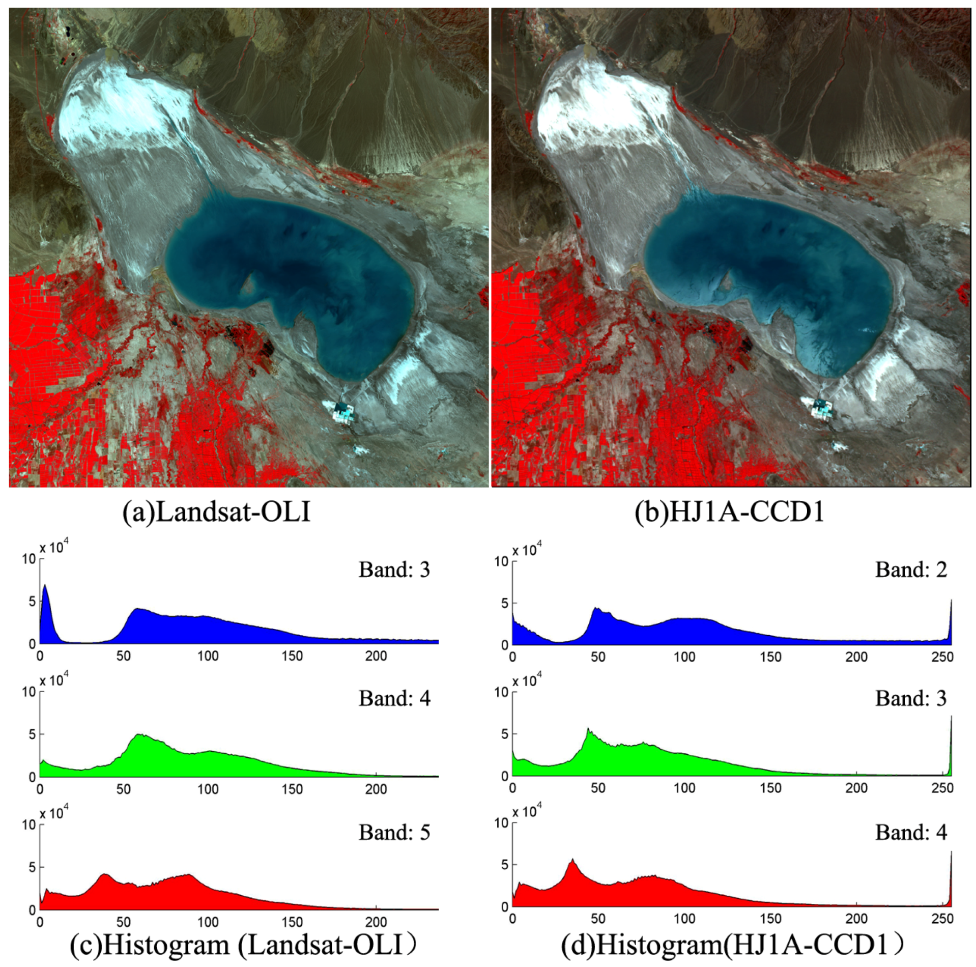
Just as in the NDVI suitability verification experiment, we selected Landsat-OLI (LC81460292014200LGN00.tar.gz) and HJ1A-CCD1 (HJ1A-CCD1-48-60-20140719-L20001179584.tar.gz) images separately as the experimental data; the images were obtained in northwest China, on 19 July 2014. After atmospheric correction and resizing, a subset of each image area (2000 pixels × 2000 pixels) was extracted in a region of water cover zones (
Figure 9). Their reflectance images are as shown in (
Figure 9a,b) (stretching gray scale range to 0–255 for display enhancements), and corresponding histogram graph of each image was as shown in
Figure 9c,d.
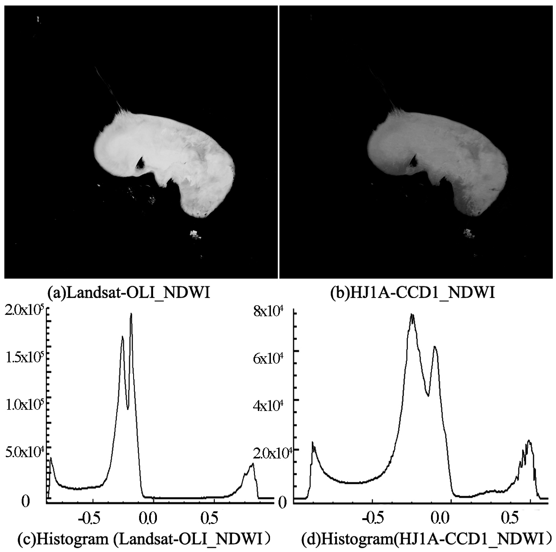
Then the NDWI of each image was calculated using the NDWI computational formula; the results are as shown in
Figure 10, and their corresponding histogram graphs are as shown in
Figure 10c,d. As can be seen in
Figure 10c,d, the gray-level distribution of Landsat-OLI NDWI histogram is relatively centralized, and that of HJ1A-CCD1 NDWI histogram is rather dispersed. For further detailed analyses, qualitative and quantitative interactive comparisons will be made.
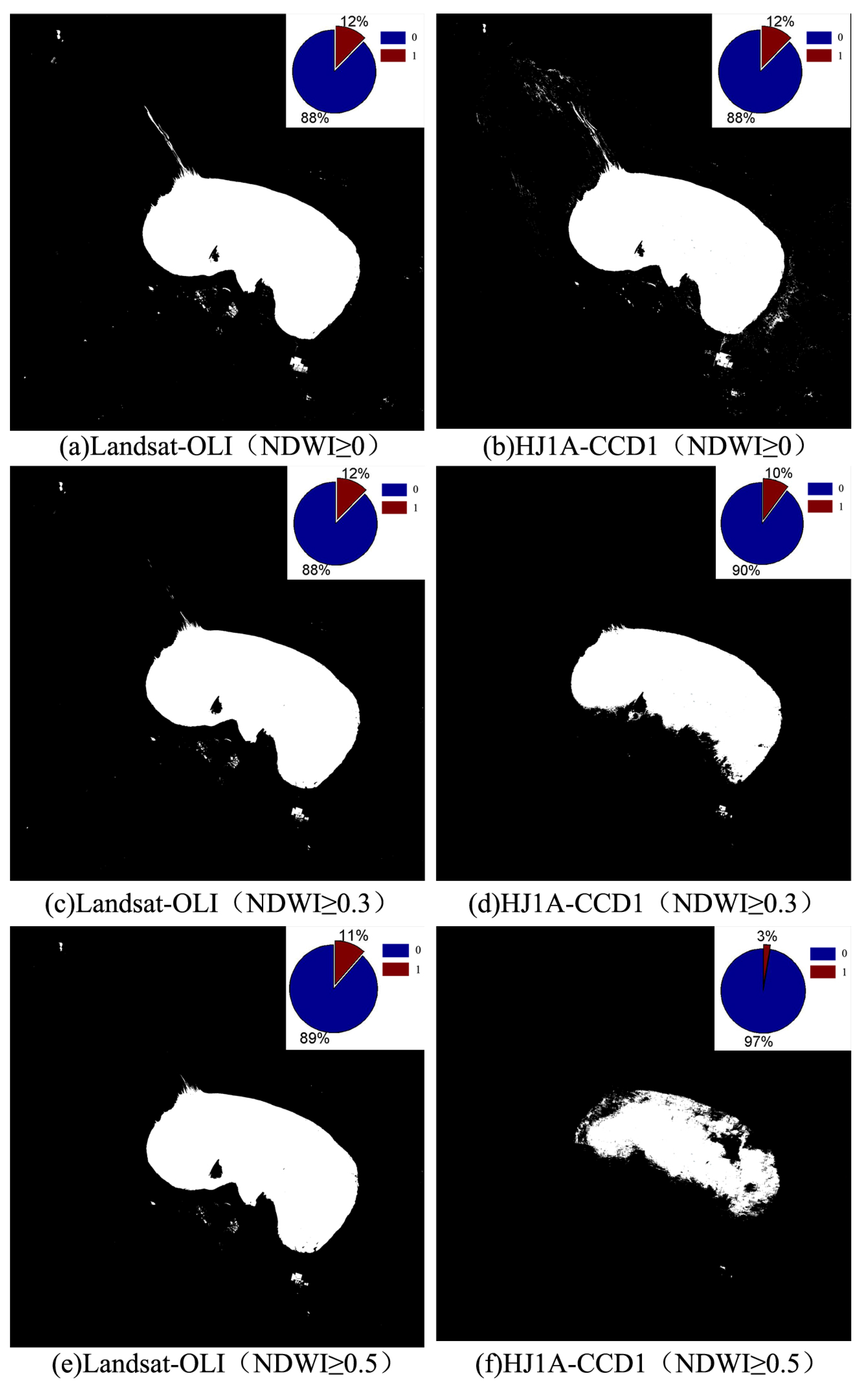
Just as in the NDVI experiment, results of the NDWI analysis for water indicate the following: low confidence (NDWI ≥ 0.0), medium confidence (NDWI ≥ 0.3), and high confidence (NDWI ≥ 0.5) (
Figure 11). In addition, in order to show the amount of water information extracted from Landsat-OLI and HJ1A-CCD1 images, the pie chart of each threshold image was obtained, and “1” denotes water information.
As shown in
Figure 11, using the same threshold, more water and water border information could be detected in the Landsat-OLI NDWI image than in the HJ1A-CCD1 NDWI image. Especially with the increase of the segmentation threshold, some water information gradually reduced or even disappear in HJ1A-CCD1 NDWI image, but that in Landsat-OLI NDWI image are still obvious. Therefore, preliminary conclusion is that the water information extracted from Landsat-OLI NDWI image is more abundant and accurate than that of HJ1A-CCD1 NDWI image. In other words, the ability of Landsat-OLI to detect water is better than that of HJ1A-CCD1. In addition, in order to quantitatively compare the degree of virtues or defects of the two NDWI images, precision would be evaluated for the NDWI threshold images using the same classified samples (
Table 11). It is worth mentioning that, the classified samples mainly include two types: (1) water samples, which were uniformly sampled from water covering area, a total of 4876 pixels; (2) non-water samples, which were uniformly sampled from grassland, bare land and other non-water areas, total 5001 pixels.
As shown in
Table 11, in each segmentation threshold, Landsat-OLI’s accuracy in identifying water and non-water areas is better than that of HJ1A-CCD1. The mean value, standard deviation, maximum value, and minimum value would be calculated in order to compare the two NDWI images on the whole (
Table 12).
As shown in
Table 12, the mean value of Landsat-OLI NDWI is a little greater than that of HJ1A-CCD1 NDWI, this may be because the lower radiance of Landsat-OLI NIR band in non-vegetation covered area, which is caused by narrower near-infrared waveband. In addition, the standard deviation value of the Landsat-OLI NDWI are greater, and this indicates that the gray scale of Landsat-OLI NDWI varies in a higher dynamic range than that of the HJ1A-CCD1 NDWI. Together with considering the histogram graph shown in
Figure 10c,d, there are three narrow peaks in Landsat-OLI NDVI, and the peak on zero right side may denote water information. As we can see, the peak on zero right side is relatively steeper, and this indicates that the water information extracted from Landsat-OLI is relatively centralized. This may be because the sharp increasement of the spectral response of green and NIR bands. As for the histogram graph of HJ1A-CCD1 NDWI, it is rather dispersed, and this further proved the weaker water and non-water distinguishing ability of HJ1A-CCD1 NDWI. It’s worth mentioning that, the maximum and minimum value of NDWI, due to the effect of image noise, they can not be used as the evaluation standard, either. Hence, the conclusion is that the Landsat-OLI NDWI includes more abundant and accurate water information, and the Landsat-OLI sensor is more sensitive for the purpose of water detection. This strongly supports the theoretical results, and proves the validity of the suitability evaluation model.
4.4. Discussions
Above all, the two experimental results showed that Landsat-OLI’s ability to detect both vegetation and water was better than that of HJ1A-CCD1, and this is consistent with our model results. This maybe benefit from the improved design of Landsat-OLI in the following aspects: (1) push-broom designment could receive stronger signals and improve signal-to-noise performance, due to the usage of long and linear arrays of detectors; (2) sharp increasement of the spectral response of green, red and NIR bands, could avoid the atmospheric absorption feature and enhance the radiometric sensitivity effectively; (3) narrower near-infrared waveband reduced mutual interference of the spectral responses among green, red and NIR bands [
29,
30]. Hence, the vegetation and water information extracted from Landsat-OLI are effectively distinguished from non-vegetation and non-water information.
In addition, similar studies showed that “in comparison with ETM+, the OLI had higher values for the near-infrared band for vegetative land cover types, but lower values for non-vegetative types” [
29]. Based on his conclusion, it can be easily deduced that (1) the Landsat-OLI NDVI is greater than that of Landsat-ETM+ in vegetation covered area, and non-vegetation covered area is just the opposite, because the reflectance value of near-infrared band is minuend in the numerator of the NDVI formula; (2) the Landsat-OLI NDWI is greater than that of Landsat-ETM+ in water covered area (non-vegetation covered area), because the reflectance value of near-infrared band is subtrahend in the numerator of the NDWI formula. That is to say, the vegetation and water distinguishing ability of Landsat-OLI is better than that of Landsat-ETM+. Compared with Landsat-ETM+ sensor, HJ1A-CCD1 sensor has almost the same width red and NIR wavebands. Except for other affecting factors, just considering the band width, we could assumed that the vegetation and water detection ability of Landsat-ETM+ and HJ1A-CCD1 is similar. Based on this assumption, our result, which shows Landsat-OLI’s ability to detect both vegetation and water was better than that of HJ1A-CCD1, is reasonable, and also indirectly proves the validity of the suitability evaluation model.
5. Conclusions
With the arrival of the big data era in Earth observation, the generation of products from multisource remote sensing data has become realizable and has been popular. In view of the insufficiency of the current data selection strategy during the process of multisource remote sensing production, this paper proposed a suitability evaluation model. Comprehensively considering the spectral characteristics of ground objects and spectra differences of each remote sensor, by means of spectrum simulation and correlation analysis, the model will enable us to obtain the PSI of each remote sensing data. In order to validate the proposed model, two typical value-added information products, NDVI and NDWI, and two similar or complementary remote sensors, Landsat-OLI and HJ1A-CCD1, were chosen, and the verification experiments were performed. The experimental results were consistent with our model calculation results, and strongly proved the validity of the suitability evaluation model.
The proposed production suitability evaluation model provides guidance for the most suitable data selection from redundant multisource remote sensing data, or selection of substitute data if data is lacking or poor quality, during the process of generating remote sensing products. It assists in the generation of standard, automated, serialized products, and will play an important role in one-station, value-added information services in the big data era of Earth observation.
However, in view of the fact that object’s spectral curve and specific production calculation formula are necessary, for those remote sensing products that need regression statistical analysis or no spectral curve consideration, such as LAI, Aerosol Optical Depth (AOD) and other complicated products, the model is powerless. In addition, with the exception of the spectrum reason proposed in this paper, there may be other factors affecting the differences of various remote sensing products. The role of other factors, such as the signal-to-noise ratio of different remote sensors, and improving the proposed suitability evaluation model for other complex products, requires further study.


