4.1.1. Scale Effect Quantified with TASI Data
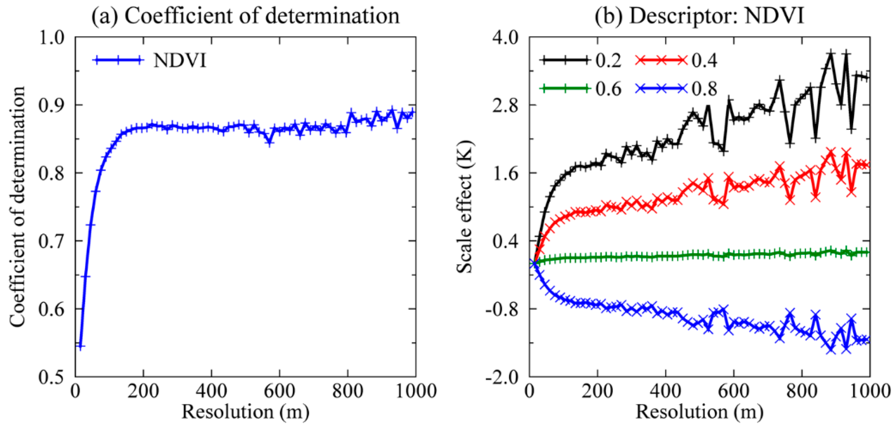
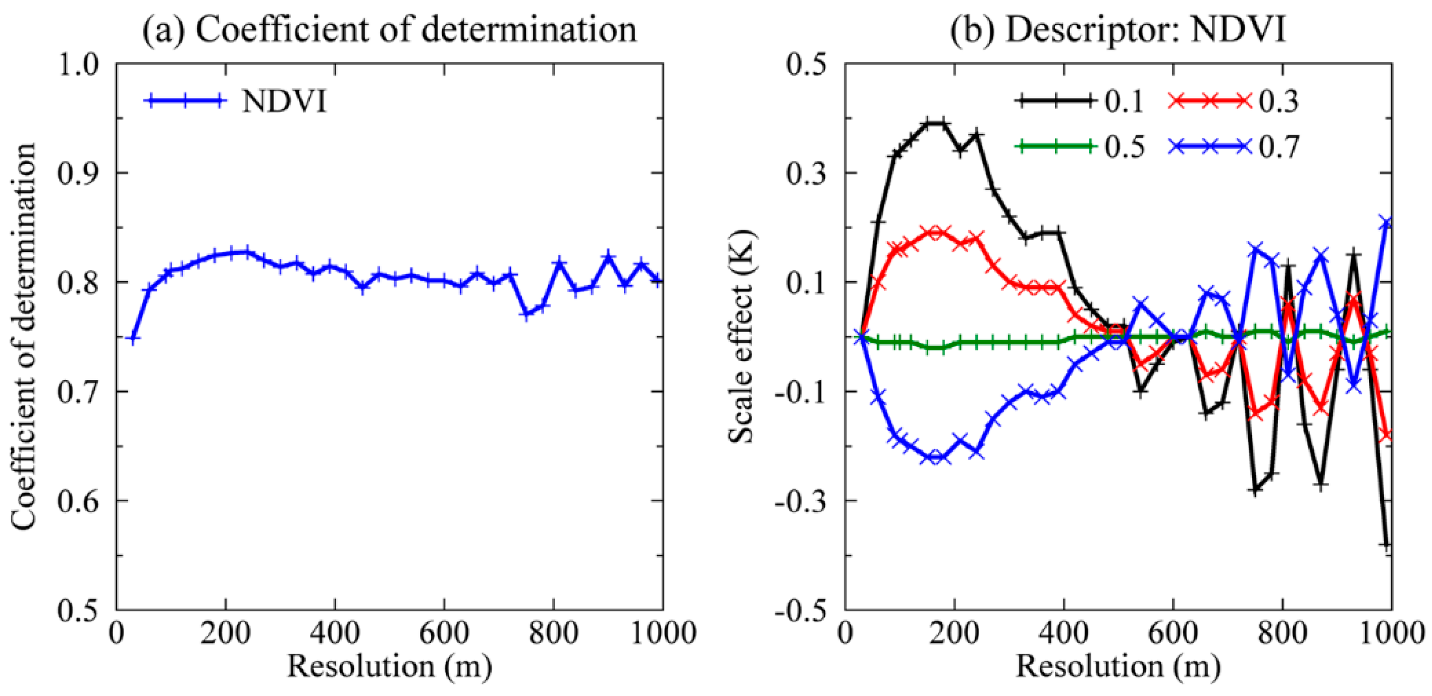
With the TASI simulated LSTs and ASTER derived parameters, the linear regression functions were trained at different resolutions. The
R2 values of the function of LST-NDVI are shown in
Figure 3a.
R2 increases from 0.545 at 15 m to 0.824 at 90 m and remains stable at approximately 0.86–0.89 after 150 m. All of the regressions are significant at the 0.001 level. Higher regression accuracy is obtained at resolutions that are coarser than 15 m due to having fewer pixel outliers. In contrast, the function of LST-FVC yields lower regression accuracy:
R2 increases from 0.530 at 15 m to 0.803 at 90 m and is ~0.84 after 150 m, which demonstrates that FVC is less capable of explaining the spatial variation of LST than NDVI in this study area on 10 July. Selecting the surface albedo as the second descriptor contributes only a slight increment to the regression accuracy.
Equation (9) demonstrates that the LST-descriptors relationship in the linear DisTrad model is scale-invariant only when Equation (1) the values of the descriptors are equal to the mean values of all of the selected pixels at the target resolution or Equation (2) the slopes at the native and target resolutions are equal. Note that similar results can be inferred for the linear TsHARP model. To verify the validity of Equation (9) and the hypotheses in an independent way, the mean values of each parameter (i.e., LST, NDVI, FVC, and surface albedo) at different resolutions were calculated. Furthermore, the scale effect was quantified according to Equation (5) by varying NDVI from 0 to 0.9 in increments of 0.1. The quantified scale effects at four NDVI values are shown in
Figure 3b. On the one hand, the mean values of these parameters at different resolutions have ignorable changes. For example, the mean values of LST, NDVI, FVC, and albedo are 304.38 ± 0.03 K, 0.628 ± 0.0, 0.639 ± 0.0, and 0.206 ± 0.0 in the range of 15 to 90 m, respectively. Thus, the transformation of Equation (5) to Equation (9) is valid. On the other hand,
Figure 3b demonstrates that the scale effect when NDVI = 0.6 is ignorable (~0.1 K) because 0.6 is close to the mean value of NDVI; the scale effect increases when NDVI deviates from the mean value. Thus, it is reasonable to infer that the scale effect in the LST downscaling increases over heterogeneous surfaces. A closer look at
Figure 3b further demonstrates that the scale effect is positive when NDVI is lower than the mean value, which reveals that the scale effect has a positive contribution to the downscaling error, and vice versa. Moreover, the scale effect also depends on the ratio of the native resolution to the target resolution. The fluctuations for resolutions that are coarser than 510 m are induced by the pixels that are located near the boundary of the oasis and its surrounding desert. The independent verification based on Equation (5) confirms the validity of Equation (9) and the hypotheses. Although the finding from the case when FVC acts as the descriptor is not shown here, similar results are also found.
In addition to GRM, the optimal regression functions LRM-MCD and LRM-LPR were trained. As demonstrated by
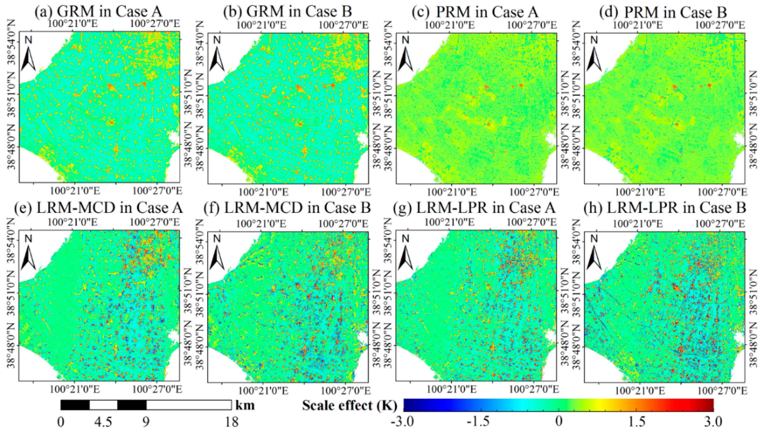
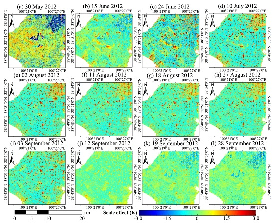
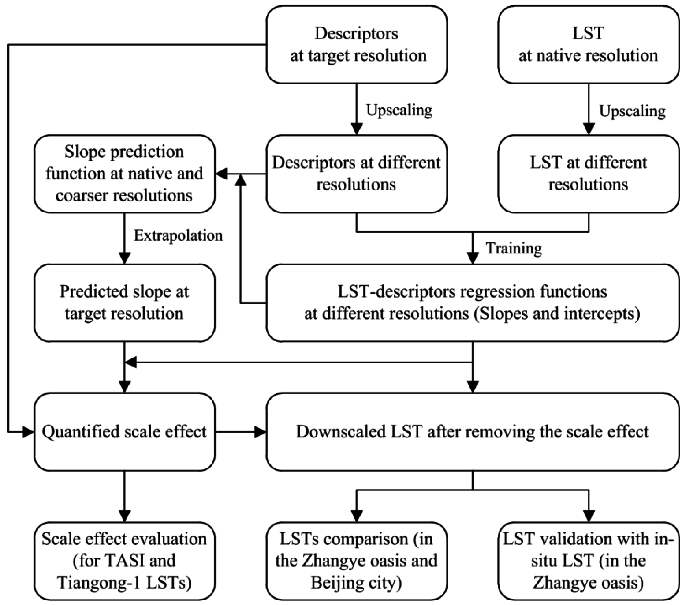
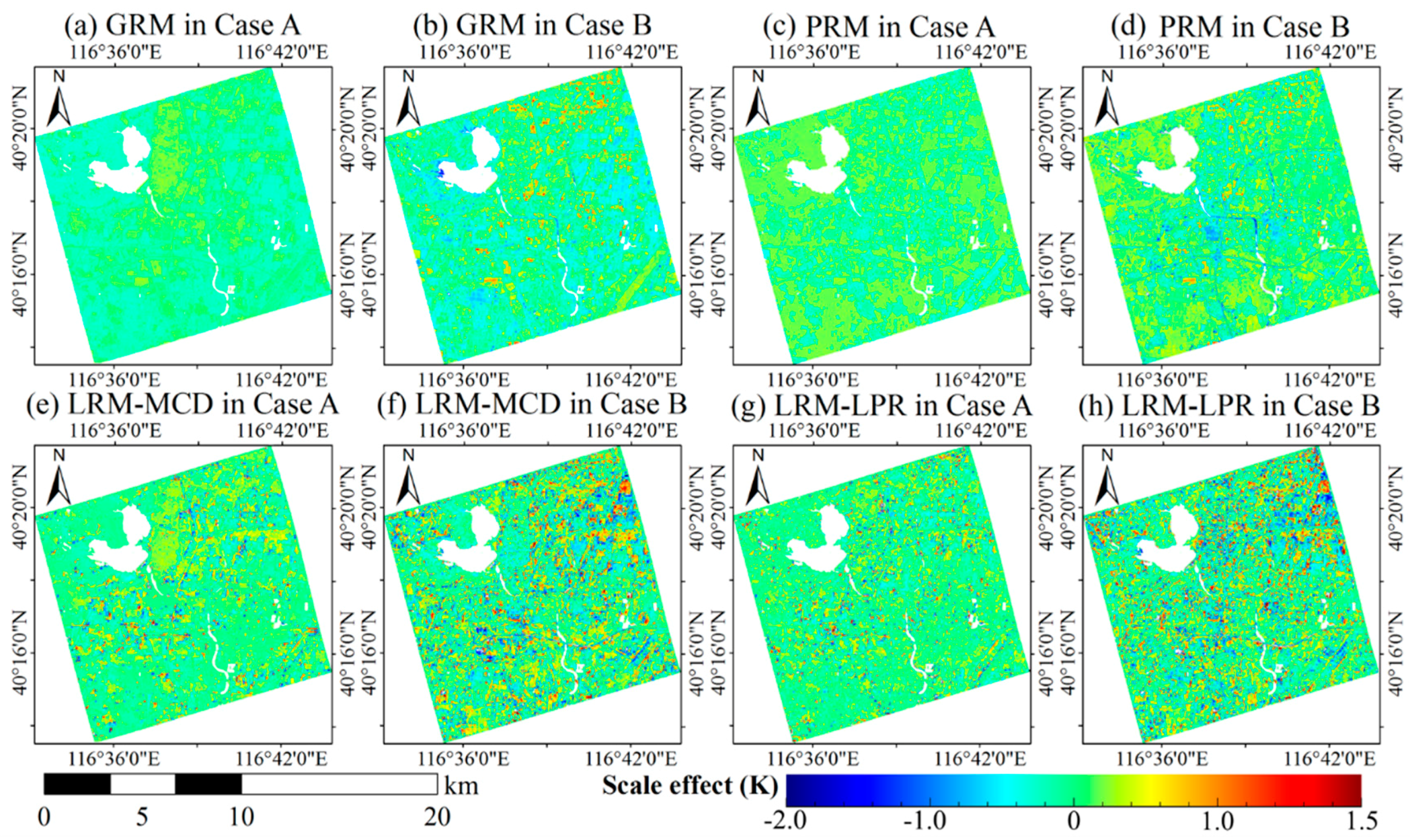
R2, the trained functions have good accuracies and are significant at the 0.001 level. The scale effects in LRM-MCD and LRM-LPR were quantified according to Equation (9), because the invariant mean values of the LST and descriptors can be guaranteed. However, PRM exhibits exceptions on two aspects. First, no regression function with acceptable accuracy was obtained when NDVI < 0.2, due to the weak ability of NDVI to explain the LST variation over barren or lowly vegetated surfaces; thus, the regression function of GRM was utilized instead. Second, the mean values of the LST and descriptors vary according to the resolution because the spatial extents that provide the pixels in training the regression functions are different at the native and target resolutions. Thus, the scale effect in PRM was quantified according to Equation (5). The spatial distributions of the scale effects in all of the models are shown in
Figure 4 by images.
As shown in
Figure 4, the scale effect mainly ranges from −0.5 to 1.5 K for GRM, with negative contributions appearing over vegetated surfaces and positive contributions over built-up and barren surfaces; these results confirm the finding from
Figure 3b. The scale effect for PRM is positive for most of the surfaces. No evident differences are found between the quantified scale effects in Cases A and Case B for GRM or PRM. Compared with GRM and PRM, the scale effects of LRM-MCD and LRM-LPR are more significant, and they range from −3.0 to 3.0 K (
Figure 4e–h). The spatial distribution of the scale effect is more irregular than on GRM and PRM, which is mostly due to the varying optimal window size for each pixel. The scale effects are closed to zero over most of the agricultural surfaces, which suggests that the local models are more capable of avoiding the scale effect over this type of surface. Several north-south linear patches suffer more from the scale effect. This phenomenon is probably induced by the mosaic of the TASI LST stripes.
The downscaled TASI LSTs were evaluated. At the 15-m resolution, the downscaled LSTs from all of the models with the scale effect retained have very similar MBD and RMSD values: MBD ranges from 0.01 K to 0.04 K, which indicates that no systematic difference exists, and RMSD ranges from 3.26 K to 3.33 K. The large RMSD are caused by the co-registration error between the ASTER derived descriptors and the TASI LST. At the 90-m resolution, the downscaled LSTs that have been upscaled back to 90 m also yield no systematic difference, and the RMSD values are approximately 1.0 K. The Q values are approximately 0.96, which demonstrates that good image qualities have been obtained. With regard to the scale effect being removed, the downscaled LSTs from GRM and LRM possess slight improvements in their accuracies; for PRM, the downscaling LSTs exhibit deteriorated accuracies. Removing the scale effect shows no evident influences on the Q values.
In contrast to GRM, PRM and LRM show no evident advantages in LST downscaling in our study area. In actual applications, GRM is the simplest to implement [
13], PRM could have difficulty in obtaining an accurate regression function when NDVI < 0.2, and LRM is extremely time-consuming in searching the optimal window to train the regression functions. Therefore, GRM is selected for further examination.
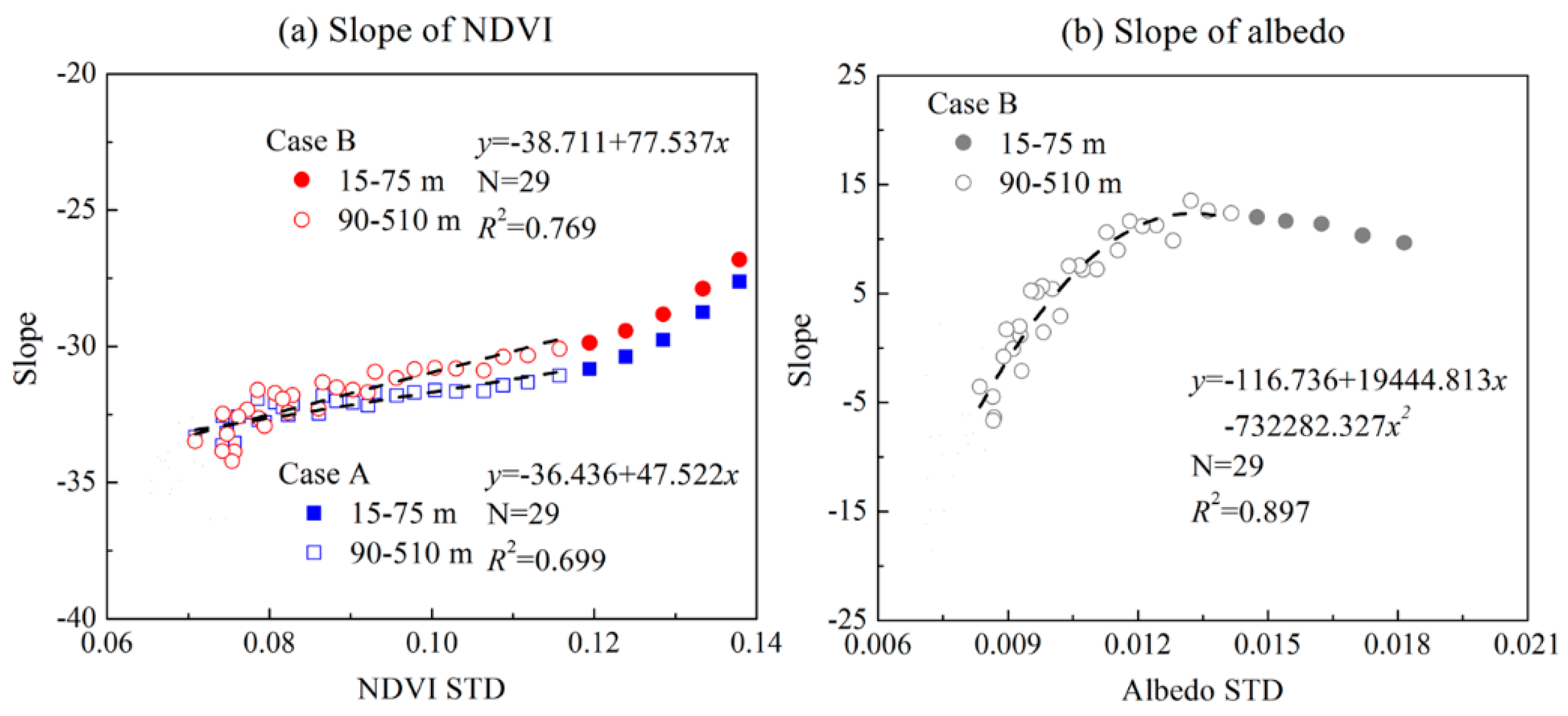
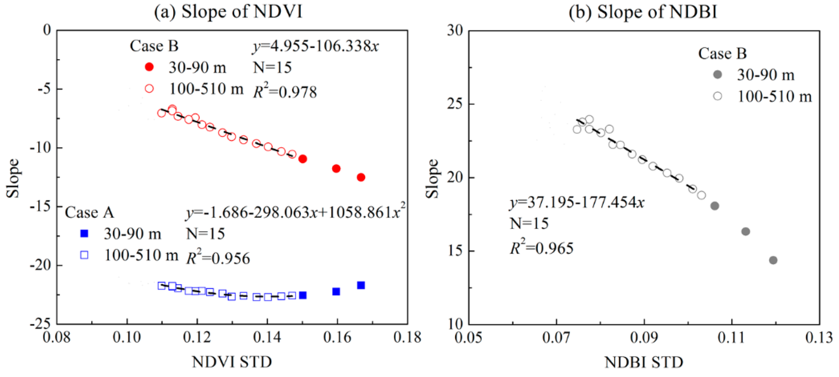
According to Equation (9), the slopes of the descriptors at the target resolution are required to quantify the scale effect, but they are unavailable in actual applications. Based on the upscaled datasets, we find that there is a significant correlation between the slopes and the standard deviations (STD) of the descriptors. As shown in
Figure 5, the slopes of NDVI in both Case A and Case B can be linearly predicted by NDVI STD in the resolution range of 510 to 90 m, although the correlation decreases at resolutions that are coarser than 510 m.
R2 values are 0.699 in Case A and 0.769 in Case B (
Figure 5a). In Case B, the slope of albedo in the range of 510 to 90 m can be predicted with a quadratic function of albedo STD, and the corresponding
R2 is 0.897 (
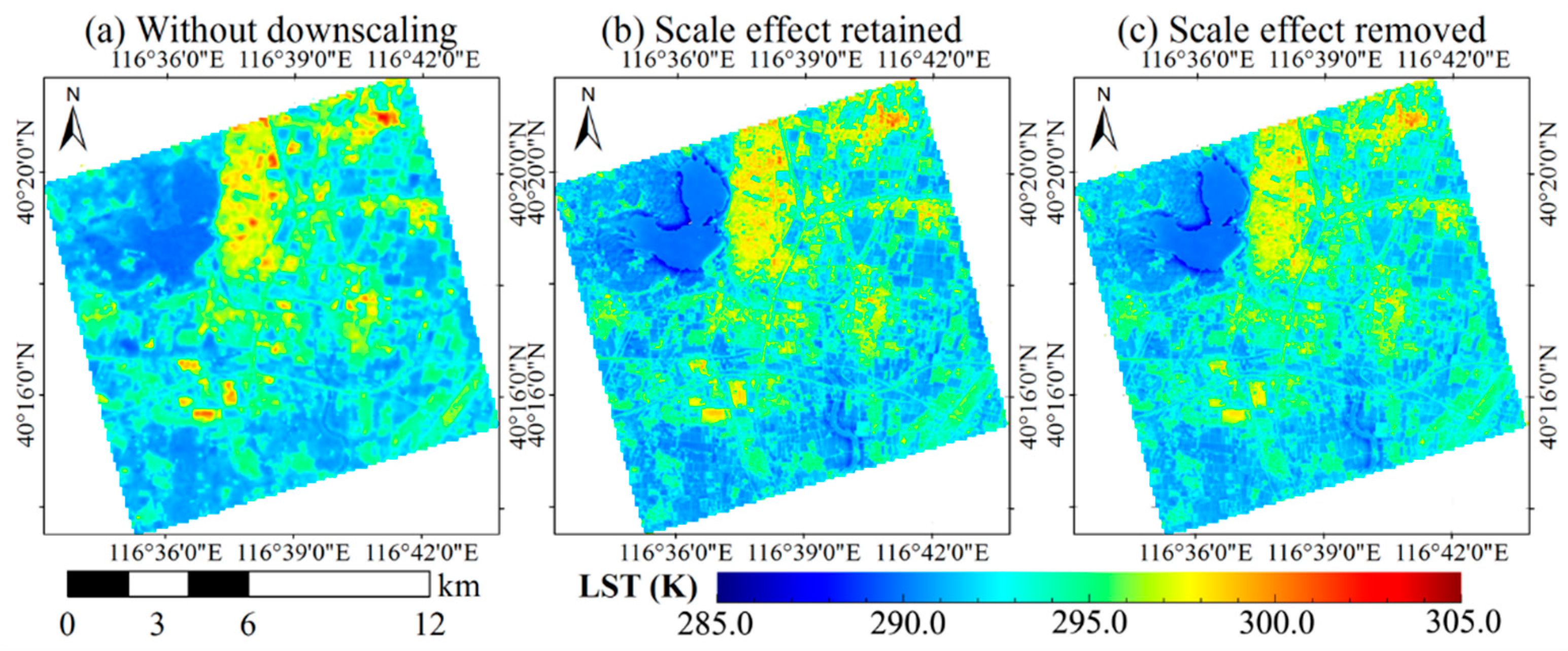
Figure 5b). These regression functions between the slopes and STDs of the descriptors can be extrapolated to resolutions that are finer than 90 m, although the correlations exhibit slight changes. As shown in
Figure 6, the estimated scale effects have very similar spatial distributions as the scale effects that are quantified with the LST at the target resolution. Nevertheless, in Case A, the estimated scale effect is weaker than that in
Figure 4 because the slope-NDVI STD function yields underestimations of the slopes in Case A (
Figure 5a); in Case B, the estimated scale effect is more significant than that in
Figure 4 due to the influences of NDVI and albedo.
4.1.2. Scale Effect Quantified with ASTER Data
To predict the slopes of the descriptors in downscaling ASTER LSTs, the correlation between the slopes and STDs were analyzed. The results are shown in
Table 1. In general, a significant correlation is found on all dates in both Case A and Case B, except for albedo in Case B on 10 July and 12 September. In both Case A and Case B, the correlation between the slope and STD of NDVI is positive, and the relationship can be sufficiently described by a linear function, which demonstrates that the slope increases at a finer resolution. This finding also confirms the existing scale effect in the LST downscaling. The slope of albedo also correlates to albedo STD, although the forms of the functions are diverse on different dates. A closer look at
Table 1 shows that the slopes of NDVI in Case A and Case B are similar from 15 June to 12 September, during which the correlations between the slope and STD of albedo are relatively weak. One reason is that the surface albedo is less capable of explaining the spatial variation of LST at the native resolution on these dates than on 30 May, 19 September, and 28 September. For example, NDVI and albedo, respectively, can explain 36.6% and 22.7% of the LST variation on 30 May, 48.9% and 5% on 19 September, and 23.3% and 7.2% on 28 September; the portion of the LST variation that is explained by albedo decreases to 0.1% on 10 July and 0.3% on 12 September. During this period, albedo is not a necessary descriptor.
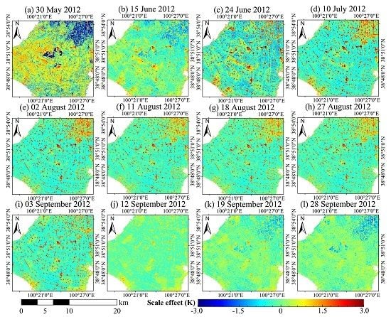
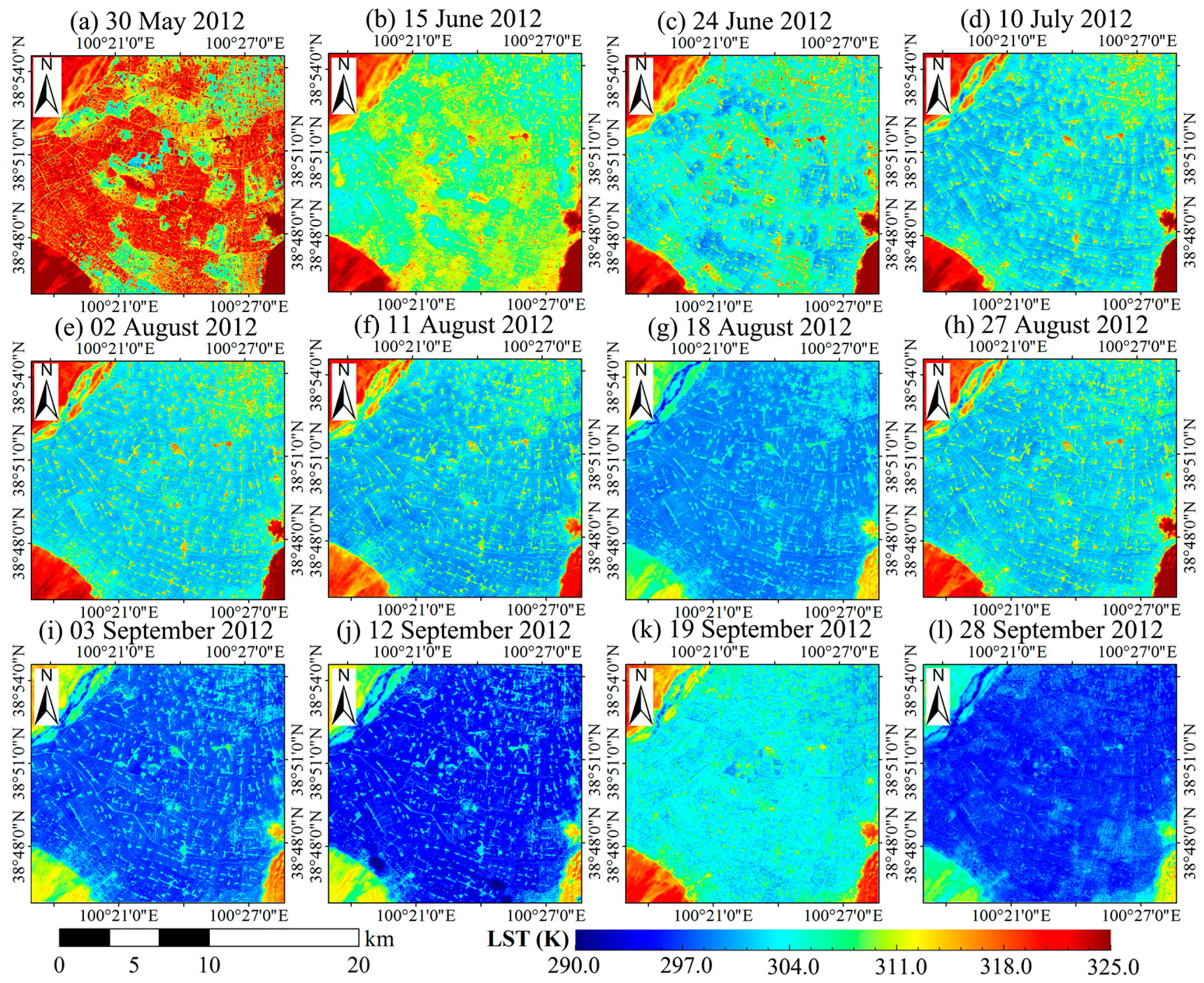
The ASTER LSTs on the 12 dates were downscaled from 90 to 15 m. The results of GRM in Case B are shown in
Figure 7. To better understand the relationship between the model performance and the crop growth, the LSTs that were downscaled from different models were validated on each date separately. Note that the results on 19 and 28 September were not validated due to a lack of in situ measured LSTs. For a fair comparison, the LSTs before downscaling were also validated. The assessments at the vegetation sites (i.e., all of the sites except for EC04) are shown in
Table 2, and those for EC04 are shown in
Table 3.
With regard to the vegetation sites, MBE and RMSE of the LSTs downscaled by GRM experience a decline first and then a rise. This trend is consistent with MBE and RMSE of the LSTs without downscaling. According to the DisTrad model and Equation (4), the errors of the downscaled LST are from the following sources. The first source is from the accuracy of the regression function and the abilities of the descriptors to explain the LST variation. In Case A, NDVI explains only 36.6%, 36.1%, 56.5%, 72.2%, and 72.0% of the LST variation on 30 May, 15 June, 24 June, 3 September, and 12 September, respectively, whereas the generally higher LST variation can be explained by NDVI in July and August. The second source is the combined influences of the surface heterogeneity and the scale mismatch between the pixel and the ground sites. The third source is the uncertainties in the LSTs at 90 m due to uncertainties that are related to the atmospheric profile, surface emissivity, and LST retrieval algorithm.
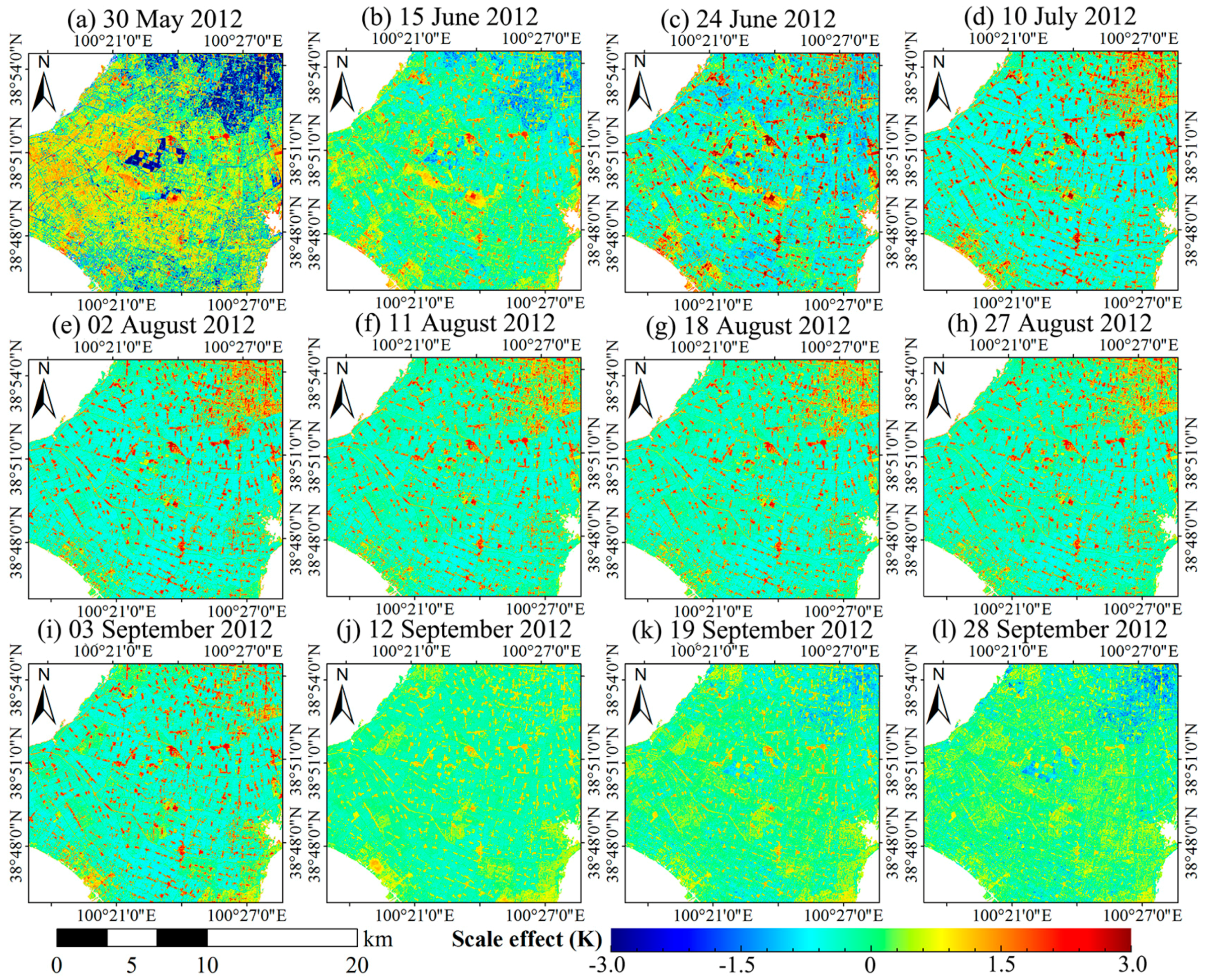
With regard to GRM in Case A, removing the scale effect cannot significantly improve the accuracy of the downscaled LST in general. One exception is 30 May, when the MBE/RMSE in Case A decrease by 1.03/0.90 K. This improvement in the accuracy results from the positive contribution of the scale effect over barren or lowly vegetated surfaces (
Figure 8) and the overestimation of the original ASTER LST (
Table 2). When the vegetation abundance increases, the scale effect becomes negative; removing the negative scale effect induces increasing MBE and RMSE because the downscaling model overestimates the LST. This phenomenon can be found on 24 June, 10 July, 18 August, 27 August, 3 September, and 12 September. An exception is 2 August: GRM underestimates the LST (MBE/RMSE: −0.51/0.84 K); thus, removing the negative scale effect improves the downscaling accuracy (MBE/RMSE: −0.07/0.60 K). When the albedo is selected as the second descriptor (i.e., Case B), the downscaling accuracies on a few dates are higher than in Case A. Removing the scale effect improves the downscaling accuracies on 30 May and 2 August.
In contrast to the vegetation sites, the original ASTER LST and downscaled LST at EC04 exhibit larger and negative errors (
Table 3). The main reasons are the scale mismatch between the ground site and its corresponding pixel and the significant overestimation of the surface emissivity due to the heterogeneous underlying surface [
40]. Compared with the original LST, the downscaling can partly mitigate the scale mismatch problem. The overall MBE/RMSE decrease from −5.15/5.58 K to −4.67/4.98 K in Case A. The albedo can further improve the downscaling accuracy. In Case B, MBE/RMSE are −4.57/4.84 K, respectively. However, removing the scale effect deteriorates the accuracies of the downscaled LST. EC04 possesses positive scale effects on all of the 12 dates. Thus, removing the positive scale effect from the underestimated LST after downscaling further underestimates the LST.
Q calculated with the original ASTER LSTs and the downscaled LSTs that have been upscaled back to 90 m are shown in
Table 4. Q demonstrates that GRM in both Case A and Case B can capture the LST spatial patterns in the study area. On a few dates, selecting albedo as the second descriptor contributes to a slight improvement on the downscaled LST images. As shown for all of the 12 dates, removing the scale effect deteriorates the qualities of the downscaled LST images, and the Q values in Case B are lower than those in Case A. On the one hand, the spatial pattern of the scale effect in GRM depends on the landscape of the study area, and densely/lowly vegetated surfaces possess negative/positive scale effects (
Figure 8). On the other hand, the downscaled LST has a similar spatial pattern as the original LST as demonstrated by the high Q values. Thus, removing the scale effect from the downscaled LST alters the spatial patterns of the LST and degrades the quality of the LST image.


