Scanning, Multibeam, Single Photon Lidars for Rapid, Large Scale, High Resolution, Topographic and Bathymetric Mapping

Abstract

Several scanning, single photon sensitive, 3D imaging lidars are herein described that operate at aircraft above ground levels (AGLs) between 1 and 11 km, and speeds in excess of 200 knots. With 100 beamlets and laser fire rates up to 60 kHz, we, at the Sigma Space Corporation (Lanham, MD, USA), have interrogated up to 6 million ground pixels per second, all of which can record multiple returns from volumetric scatterers such as tree canopies. High range resolution has been achieved through the use of subnanosecond laser pulsewidths, detectors and timing receivers. The systems are presently being deployed on a variety of aircraft to demonstrate their utility in multiple applications including large scale surveying, bathymetry, forestry, etc. Efficient noise filters, suitable for near realtime imaging, have been shown to effectively eliminate the solar background during daytime operations. Geolocation elevation errors measured to date are at the subdecimeter level. Key differences between our Single Photon Lidars, and competing Geiger Mode lidars are also discussed.

1. Introduction

Conventional mapping lidars fall into two broad categories—discrete return lidars and digitized waveform lidars. As can be seen from Figure 1, discrete return lidars provide one or more event times (ranges) where the received intensity exceeds a common threshold but there is no other vertical spatial information in between. Digitized waveform lidars, on the other hand, provide intensity information over the entire vertical structure but each point in the profile represents the sum of the returns over the transverse extent of the laser beam at a given range. Digitized waveform lidars typically require hundreds of detected photons and are most useful when mapping areas where multiple vertical returns are expected from complex semi-porous structures such as tree canopies, very rough terrain, or even manmade structures. The earliest version of our Single Photon Lidar (SPL), the NASA “Microaltimeter” described in Section 2.1, used a single beam with only 2 microjoules of energy per pulse and a multistop timing receiver to record tree canopies and the underlying terrain from altitudes above ground level (AGLs) as high as 7 km [1]. In effect, it was a degraded version of a digitized waveform lidar and, if one were to repeat the low energy measurements many times and create histograms versus range, one would expect to generate a profile comparable to that of the waveform digitizer. On the other hand, individual photon returns originate at a specific scattering point within the canopy and, unlike waveform lidars, are isolated from nearby returns which occur at the same range but originate from other points within the transverse extent of the laser beam. Later SPL generations, to be described in this article, take advantage of the receiver’s single photon sensitivity by splitting a single laser beam into 100 beamlets, arranged in a 10 × 10 array. Each beamlet is then imaged onto a pixel in a matching 10 × 10 array detector which, in turn, is input to a timing channel able to record multiple stop events per pixel with few picosecond accuracy. This alone increases the surface measurement rate by two orders of magnitude relative to the laser fire rate. When the source laser is operating at tens of kHz, surface measurement rates of several megapixels per second are achieved. Furthermore, our lidars are designed to provide a mean of 3 photoelectrons per pixel for green vegetation (10% surface reflectance at 532 nm) when operated at their design AGL. Thus, a tree canopy will result in approximately 300 photoelectrons being detected per pulse, a number not dissimilar to some Digitized Waveform lidars, but with the added benefit that the transverse coordinates of the scattering points are identified as well as the range, thereby providing more detailed 3D vs. 1D maps of the canopy. It must also be mentioned that a competing single photon sensitive technique based on Geiger Mode Avalanche Photodiode Arrays has also recently been introduced to the commercial market, by Harris Corporation and their different characteristics will be discussed in Section 5.

Single photon sensitive 3D imaging lidars have multiple advantages relative to conventional multiphoton lidars. They are the most efficient 3D imagers possible since each range measurement requires only one detected photon as opposed to hundreds or even thousands in conventional laser pulse time of flight (TOF) or waveform altimeters. Their high efficiency enables orders of magnitude more imaging capability (e.g., higher spatial resolution, larger swaths and greater areal coverage). In our Single Photon Lidars (SPLs), single photon sensitivity is combined with a 1.6 nanosecond receiver recovery time (often referred to as “deadtime”), and is therefore capable of recording returns from objects differing by only 24 cm in range. This enables our lidars to operate effectively in daylight and to penetrate semi-porous obscurations such as vegetation, ground fog, thin clouds, etc. Furthermore, unlike most lidars which operate at the fundamental Nd:YAG wavelength of 1064 nm in the Near InfraRed (NIR), the SPL 532 nm operating wavelength is highly transmissive in water, thereby permitting shallow water bathymetry and 3D underwater imaging. In order to enhance the range resolution of SPLs, FWHM laser pulsewidths on the order of 100 to 700 picoseconds are used whereas conventional lidars typically employ few nanosecond pulsewidths and rely on large photon counts from the surface to improve the precision of the range measurement.

On the other hand, sensitivity to single photon surface returns also make SPLs sensitive to background noise originating from: (1) dark counts from the sensitive detectors; (2) solar backscatter from the surface being examined and the intervening atmosphere within the pixel field of view (FOV); and (3) laser backscatter from the atmosphere within the selected range gate. Sources (1) and (3) occur during both day and night mapping operations but are relatively inconsequential compared to the solar scatter encountered in daylight. Conventional lidars have multiphoton thresholds and therefore do not record single photon solar or dark count events. The solar count rate per pixel is proportional to the pixel FOV and the receive telescope aperture [2]. Thus, shrinking the pixel FOV not only reduces the solar count rate in an SPL, but it also improves the horizontal spatial resolution of the lidar. Furthermore, the single photon sensitivity of the receiver allows a substantial reduction in receive aperture, thereby further reducing the number of noise events [2]. Finally, these sources have been effectively mitigated through the use of highly effective noise filtering algorithms such as the Differential Cell Count method [2]. For further insights into the characteristics and relative merits of the various lidar types, the reader is referred to the book chapter by Harding [3].

In Section 2 of this paper, we present an overview of our multibeam scanning airborne SPLs to date and the manner in which they have been adapted to operate at higher AGLs and cruise speeds for faster areal coverage. In Section 3, we briefly discuss progress in developing fast and autonomous data editing software for extracting surface data from the solar background during daylight operations and the potential for near real time 3D image generation for cockpit display and/or transmission to a ground station. Section 4 provides examples of different data types in order to demonstrate their relevance to applications such as large scale surveying, Cryospheric studies, forestry, and shallow water bathymetry. Section 5 discusses the relative advantages and disadvantages of SPL vs Geiger Mode technology, which was developed over two decades by the US military but has recently been introduced into the civilian market by Harris Corporation. Finally Section 6 provides some concluding remarks about ongoing research and field activities to provide improved data products, including the possibility of globally contiguous mapping of planets and moons from orbital altitudes between 100 and 500 km.

2. SPL Instrument Overview and Heritage

2.1. NASA “Microaltimeter”

NASA’s Microlaser Altimeter or “Microaltimeter” provided the first airborne demonstration of a scanning Single Photon Lidar (SPL) in early 2001 [1]. Although several natural properties (e.g., atmospheric transmission, natural surface reflectivity, solar background) favor use of the fundamental Nd:YAG wavelength at 1064 nm, 532 nm was chosen as the operating wavelength for technology reasons (e.g., higher efficiency COTS array detectors with nanosecond recovery times, high transmission narrowband filters, etc.) [2]. A side benefit of the choice was the instrument’s demonstrated ability to see the bottom of the Atlantic Ocean off the coast of Virginia to a depth of about 3 m from an altitude of 4 km. The lidar also successfully penetrated tree canopies to see the underlying surface. The 532 nm operating wavelength has been maintained through the successive generations of lidar described here.

With less than 2 microjoules per pulse at a laser repetition rate of 3.8 kHz (~7.6 mW average power), the single beam “Microaltimeter” produced high resolution 2D profiles or low resolution 3D images over narrow swaths (~60 m) while operating mid-day at altitudes up to 6.7 km. Although the passively Q-switched, microchip Nd:YAG laser was incredibly small (~2.3 mm in length) and pumped by a single diode laser, the overall lidar was quite large and flew in the cabin of NASA’s P-3 aircraft. Nevertheless, this 1st generation system demonstrated the feasibility of: (1) making accurate surface measurements with single photon returns under conditions of full solar illumination; and (2) developing high resolution spaceborne laser altimeters and imaging lidars operating from orbital altitudes of several hundred km [2].

2.2. Second Generation SPL (“Leafcutter”)

From 2004 to 2007, Sigma developed its first multibeam Single Photon Lidar (SPL), dubbed “Leafcutter” [4]. Leafcutter, shown in Figure 2, was designed to fit into the nose cone of an Aerostar Mini-UAV and provide contiguous decimeter resolution images on a single overflight from AGLs between 1 and 2.5 km, depending on surface reflectance. The overall system, including GPS receiver and Inertial Measurement Unit (IMU), consisted of two units (optical bench and electronics box), weighed 33 kg, occupied a volume of less than 0.07 m³, and drew ~170 W of aircraft 28 VDC prime power. In parallel to this activity, Sigma Space also provided hardware and technical support to two other single photon systems, i.e., the University of Florida’s Coastal Area Tactical-Mapping System or CATS [5,6] and NASA Goddard Space Flight Center’s Slope Imaging Multi-polarization Photon-counting Lidar or SIMPL [7].

A 10 × 10 square array of 100 beamlets was generated by passing the 140 mW COTS laser transmitter beam through an 80% efficient Diffractive Optical Element (DOE). Each beamlet contained approximately 1 mW of laser power in a 22 kHz stream of 700 ps FWHM, 50 nJ pulses. At the design AGL of 1 km, the interbeam spacing between beamlets was 15 cm, and the ground images of the beamlets were optically matched to a COTS 10 × 10 segmented anode, MicroChannel Plate PhotoMultiplier Tube (MCP/PMT). The individual anode outputs were then input to an inhouse multichannel timing receiver with an RMS timing/range precision of 23 ps/3.4 mm. Most importantly, the detector/receiver subsystem can record the arrival times of multiple, closely-spaced photons per channel with an event recovery time of only 1.6 ns. This made Leafcutter impervious to shut-down by random solar events and also permitted multiple returns per channel from semi-porous volumetric scatterers such as tree canopies. The solar noise per pixel was kept to a minimum through the use of a 0.3 nm FWHM spectral filter, a small receive telescope 7.5 cm in diameter, and a Field-of-View (FOV) limited by the nominal 15 cm × 15 cm ground pixel dimension, which over a nominal 1 km range amounts to a solid angle of only 2.2 × 10⁻⁸ steradians per pixel.

The use of the 10 × 10 beamlet array increased the surface measurement rate by two orders of magnitude to 2.2 million multistop pixels per second. The array also allowed high resolution contiguous maps of the underlying surface to be generated on a single overflight at relatively high air speeds with modest scan speeds on the order of 20 Hz or less, which were easily achieved with the relatively small receive aperture. A further advantage is that, for each of the spatially separated pixels, there is only one pulse in the air per measurement until the surface slant range exceeds 6.8 km. This is in contrast to some commercial linear mode lidar designs which attempt to achieve higher measurement rates using a single beam at very high repetition rates (~200 kHz). At these frequencies, complications associated with multiple pulses in flight begin at surface slant ranges an order of magnitude smaller (~700 m).

Leafcutter employs a dual wedge optical scanner, which is common to both the transmitter and receiver. By adjusting the rotation direction and/or the rotational phase differences between the two wedges, one can generate a wide variety of scan patterns including: (1) linear scans at arbitrary orientations to the flight line (see Figure 2); (2) conical scans of varying radius; (3) spiral scans, etc. Maximum angular offset from nadir when the two wedges are coaligned is 14 degrees, corresponding to a maximum swath of about 0.5 km at a 1 km AGL (Altitude above Ground Level). During rooftop testing, a “3D camera mode”, i.e., a rotating line scan, shown in Figure 2, was used to generate a contiguous high resolution 3D image within a circular perimeter.

NASA funded several test flights to assess SPL capabilities in the areas of biomass (forest cover), cryospheric, and bathymetric measurements. A collage of sample results from Leafcutter is presented in Figure 3. A second similar unit, labeled “Icemapper”, was later delivered to the University of Texas at Austin to participate in Antarctica ice-mapping missions. As can be seen in Figure 3, the 532 nm operating wavelength allowed bathymetry to a depth of 15 m in glacier melt ponds and to about 4 m depth in the more turbid waters of the Chesapeake Bay near Annapolis, MD, USA. Note also that the surface of the melt pond is well defined even at a beam incidence angle of 14 degrees, indicating that Lambertian scattering from water molecules at and just below the water surface, rather than specular reflections, are creating the surface signal. Furthermore, what appears to be excess noise at the pond bottom is in reality variations in the bottom elevation when the entire pond is viewed from the side.

2.3. NASA Mini-ATM

Subsequent to the highly successful cryospheric results obtained by Leafcutter, NASA funded development of an even smaller 100 beamlet system, imaged onto 25 pixels (4 beamlets per pixel), to potentially replace the highly successful, but much larger and heavier, P-3 based Airborne Topographic Mapper (ATM), which had mapped the Greenland ice sheets for many years. “Mini-ATM” reused most Leafcutter components and subsystems but was light-weighted and reconfigured to fit into the payload bay of a Viking 300 Micro-UAV (see Figure 4). The current version of the multiphoton ATM lidar has a nominal spacing between measurements of 2.5 m (0.16/m² point density) which generally met the needs of Cryospheric scientists tracking changes in ice sheet thickness in support of NASA Global Climate Change programs. Thus, to maximize swath and thereby minimize the time required to map large ice sheets, Mini-ATM features a 90° full conical holographic scanner. For the nominal Viking 300 velocity of 104 km/h and altitude ceiling of 3 km, the system is designed to autonomously map up to 600 km²/h with a mean measurement point density in excess of 1.5/m²—a density about 10 times higher than that achieved by the current man-assisted ATM. Including a dedicated IMU, Mini-ATM has a cubic configuration (see Figure 4) with a volume of 0.03 m³, weighs 12.7 kg, and consumes ~168 W of 28 VDC prime power. Mini-ATM completed its first successful test flight in a manned aircraft over California’s Mojave Desert in October 2010.

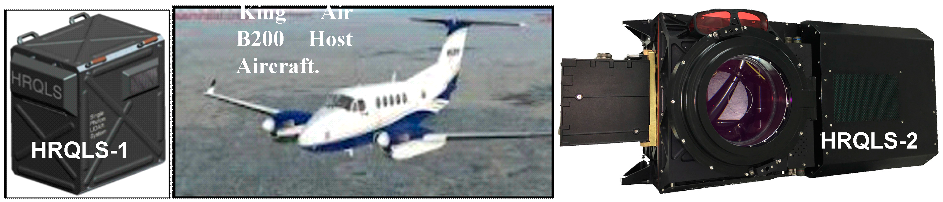
2.4. High Resolution Quantum Lidar System (HRQLS 1 and 2)

Development of the moderate altitude High Resolution Quantum Lidar Systems, (HRQLS-1) and its upgraded successor, HRQLS-2, were self-funded by Sigma and are shown in Figure 5. Both systems follow the same design philosophy as “Leafcutter”, i.e., 100 beamlets in a 10 × 10 array, but the spacing between pixels at the ground is increased to 50 cm at their nominal AGLs as described in

Table 1. Summary table of design and performance properties for the current suite of Sigma scanning SPL lidars.

	Low Altitude SPLs		Medium Altitude SPLs		High Altitude SPLs
Instrument Name	USAF “Leafcutter”	NASA Mini-ATM	HRQLS-1	HRQLS-2	HAL
Prototype Completion Dates	2007	2010	2013	2016	2012
Units/Customers	2/USAF & Univ. of Texas	1/NASA	1/Sigma	6/Sigma	3/DoD
Primary Application	Military Prototype & Antarctic Cryosphere	Greenland Cryosphere	Civilian Surveying and mapping, Biomass Measurement, Bathymetry, Military Surveillance		Military Surveillance
Design Platform	Aerostar Mini-UAV	Viking 300 UAV	King Air	King Air	Various
# beams/pixels, Np	100/100	100/25	100/100		100/100
Wavelength	532 nm		532 nm		532 nm
Laser Repetition Rate, fqs	22 kHz		25 kHz	60 kHz	32 kHz
Laser Pulse Width (FWHM)	0.7 ns		0.7 ns	0.5 ns	0.1 ns
Laser Output Power	0.14 W		1.7 W	5 W	15 W
Maximum Measurements/s	2,200,000	550,000	2,500,000	6,000,000	3,200,000
Multiple Return Capability	Yes		Yes		Yes
Pixel Recovery Time	1.6 ns		1.6 ns		1.6 ns
RMS Range Precision	5 cm		5.7 cm	4.8 cm	3.6 cm
Telescope Diameter	7.5 cm		7.5 cm	14 cm	14 cm
# Scanner Wedges	2	DOE	2	1 Wedge or DOE	1 Wedge
Scan Width (FOV)	Variable 0° to 28°	Fixed 90° cone	Variable 0° to 40°	20°, 30°, 40° or 60°	Fixed 18°
Nominal A/C Velocity, vg	161 km/h	104 km/h	370 km/h		370 km/h
Design AGL	1 km	2.5 km	2.3 km	3.4 km	7.6 km
Nominal AGL Range, h	1.0 to 2.5 km	0.55 to 3 km	2 to 3 km	3 to 5.5 km	6 to 11 km
Swath, S	0.0015 to 1.247 km	1.1 to 6 km	0.005 to 2.184 km	1.058 to 6.351 km	1.901 to 3.484 km
Areal Coverage, Svl	0.242 to 201 km2/h	114 to 624 km2/h	2 to 808 km2/h	391 to 2350 km2/h	703 to 1289 km2/h
Mean Measurement Attempts per m2 per pass, Dm	39 to 32,795/m2	3 to 17/m2	11 to 4865/m2	9 to 55/m2	9 to 16/m2
# of Modules	2	1	1 (rack-mounted)		1 (rack mounted) 1 (pod mounted)
Instrument Volume/Dimensions	0.071 m3	0.027 m3 Quasi-cube (0.3 m)	0.26 m3 48 × 64 × 84 cm3	0.139 m3 82.5 × 48.25 × 35 cm3	0.52 m3 49 × 64 × 163 cm3
Weight	33 kg	13 kg	57 kg	68 kg (sensor head) 22 kg (e-rack)	113 kg (est.)
Prime Power (28VDC)	266 W	~168 W	555 W	700 W	<900 W (est)
Status	2 Delivered	1 Delivered	1 Operational	2 Operational, 4 in fab	2 Delivered, 1 in fab

. The primary technical goal of HRQLS-1 was to map larger areas more quickly via a combination of higher air speeds and wider swaths while still permitting the experimenter to tailor the measurement point density to fit his or her individual needs. The wider swath is achieved by: (1) flying at a higher altitude; (2) increasing the laser power to about 1.7 W to compensate for the larger 1/R² signal loss (where R is the slant range to the target); and (3) increasing the maximum half-cone angle of the scanner to 20 degrees.

In order to accommodate a large range of measurement point densities, HRQLS-1 also features an external dual wedge scanner at the output of the 7.5 cm diameter telescope, which allows a range of full cone angles between 0 and 40 degrees, resulting in swath widths as small as 5 m and as large as 1.66 km at the nominal 2.3 km AGL. This feature allows measurement point density (or spatial resolution) to be traded off against swath and areal coverage. However, because of the longer pulse times-of-flight (TOFs) and high scan speeds, the images of the beamlet array become displaced relative to their assigned pixel centers unless one implements an optical TOF correction [7]. Thus, in HRQLS, annular corrector wedges are attached to each of the main scanner wedges in order to bring the transmitter and receiver FOVs into alignment at the nominal AGL. Maintaining alignment between the transmitter and receiver FOVs at different AGLs is accomplished by adjusting the angular speed of the scanner—faster for AGLs lower than nominal and slower for AGLs higher than nominal.

The upgraded HRQLS-2 was subsequently developed to allow high point density operation at AGLs above 3.1 km where FAA regulations permit more flexibility on flight lines. Instead of a dual wedge scanner, however, HRQLS-2 uses a variety of interchangeable single wedge or holographic scanners with full cone angles ranging from 20 to 60 degrees.

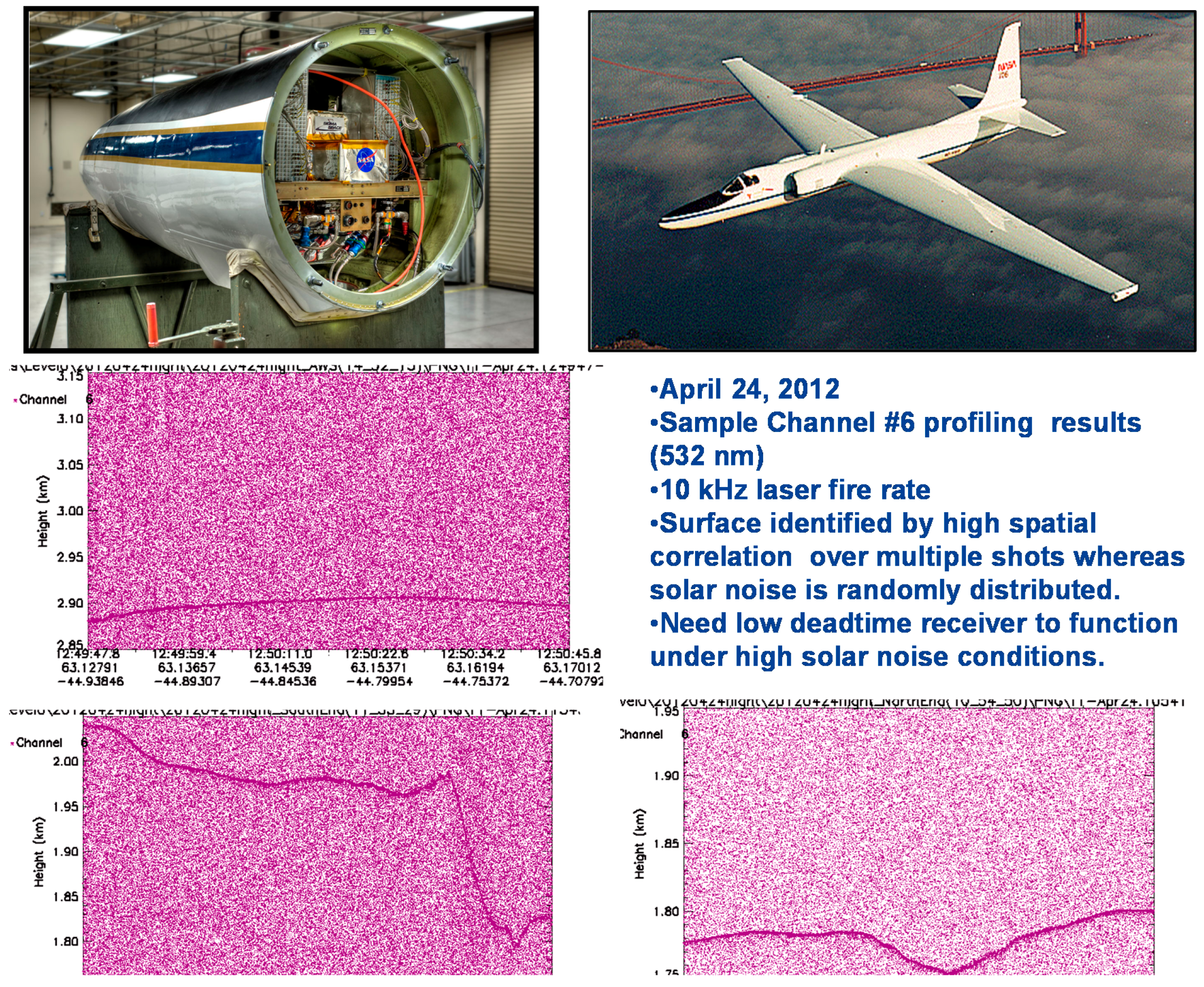
2.5. High Altitude Lidar (HAL)

Two versions of Sigma’s High Altitude Lidar (HAL) currently exist to operate from either an internal cabin or an external pod environment. HAL was designed to produce contiguous, few decimeter resolution, topographic maps on a single pass from AGLs between 6.4 and 11 km. At these high AGLs, the importance of using scanner corrector wedges to compensate for finite speed of light effects is even more crucial since the overlap between transmit beamlet arrays and detector FOVs can, under some operational scenarios, be reduced to zero with the result that no surface signals are detected.

Depending on the operating AGL, there are either 2 or 3 pulses simultaneously in flight, and this can be taken into account during data processing by simply pairing the proper start pulse with the observed stop pulses. HAL can provide contiguous maps at aircraft speeds in excess of 407 km/h. The single wedge scanner has a 9° half-cone angle. Thus, at a maximum AGL of 11 km, the swath is 3.48 km and the maximum rate of areal coverage is 1415 km²/h. The HAL images are comparable in quality and resolution to the HRQLS images in Section 4 of this paper [8].

2.6. NASA’s Multiple Altimeter Beam Experimental Lidar (MABEL)

Sigma provided all of the electronics modules, including the multichannel timing receiver, as well as key mechanical, thermal, integration, testing and flight operations support to NASA’s Multiple Altimeter Beam Experimental Lidar (MABEL) instrument, which was developed as a precursor and testbed for the Advanced Topographic Laser Altimeter System (ATLAS) SPL, scheduled to be launched in 2017 into a 500 km orbit on NASA’s second generation Ice, Cloud, and land Elevation Satellite-2 (ICESat-2) mission [9]. MABEL is a nonscanning, 24 beam (8 @ 1064 nm, 16 @ 532 nm) pushbroom lidar hosted on NASA’s ER-2 Research aircraft (see Figure 6). It has successfully demonstrated single photon surface profiling at AGLs of 20 km in both California and Greenland [10].

2.7. Summary Table of Sigma Scanning Lidar Properties

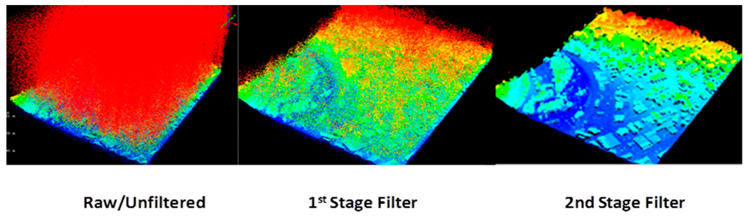
Table 1 provides a summary of the physical (Size, Weight, and Power or SWaP) and performance properties of the various scanning SPLs described in previous subsections. Dual wedge scanner systems such as “Leafcutter” and HRQLS-1 can vary the cone angle from 0° to some maximum cone angle, i.e., 28° for Leafcutter and 40° for HRQLS-1. HRQLS-2 is equipped to alternate between 4 distinct cone angles while HAL currently only has one (18° full cone angle). All of the systems can operate effectively over a range of AGLs about the “Design AGL”, which is defined as the AGL where, from Poisson statistics, the expected pixel Photon Detection Efficiency (PDE) = 1 − exp(−n_p) = 95% (mean detected photoelectrons per pixel n_p equals 3) at the largest scan cone angle over a 10% reflectance Lambertian surface (e.g., green vegetation at 532 nm operating wavelength). The per-pixel PDE is over 99% for surface reflectances greater than 15% at 532 nm (e.g., soil and dry vegetation).

By deviating from the design AGL, one can generate a greater density of measurements over a smaller swath (lower AGL) or a lower density of measurements over a wider swath (higher AGL) for faster areal coverage. When operating at the design AGL, the nominal pixel spacing at the ground is 50 cm for both HRQLS models and HAL The minimum swath in the table corresponds to the minimum cone angle from the minimum AGL while the maximum swath is obtained by using the maximum cone angle at the maximum AGL. At all AGLs at or below the design AGL, the percentage of returns from a 10% reflectance Lambertian surface is greater than 95%. At AGLs higher than the design AGL, the percentage of surface returns will decrease only slowly due to the fact that our systems are designed to operate in the highly nonlinear portion of the Poisson probability curve.

The mean number of range measurement attempts per square meter made by the lidar can be easily estimated by dividing the total number of measurement attempts by the total surface area scanned during the same time interval, i.e.,

$$D_m=\frac{N_p{f}_{qs}}{S{v}_g}=\frac{N_p{f}_{qs}}{2h{v}_g\tan \mathsf{\alpha }}$$

(1)

where N_p = 100 is the number of beamlets/pixels per pulse, f_qs is the pulse repetition rate of the laser, S is the swath width, v_g is the ground velocity of the aircraft, h is the operating AGL, and α is the scanner cone half angle. As one can easily see from Table 1, all SPL lidar models listed can meet USGS Quality Level 1 data densities (8 pts/m²) over some portion of their aircraft AGL and scan angle ranges.

The RMS instrument range errors listed in the table are computed based on a convolution of the RMS errors introduced by the laser, the detector, and the range receiver and do not include additional RMS contributions due to non-zero incidence angles of the beamlets on the surface [2]. Since all of the systems use virtually identical detectors and receivers, the small differences in RMS between systems are due to differing laser pulse widths.

3. Data Editing

Unlike conventional multi-photon lidars that nullify solar noise by operating at high detection thresholds, SPLs require a substantial amount of noise editing during daytime operations. Early in our development program, data editing approaches were implemented only after the complete point cloud (signal plus noise counts) was generated by inhouse software and viewed via a commercial program such as QT-Modeler^®. Early editing approaches often involved substantial human intervention to generate acceptably “clean” images. However, we have developed and successfully tested highly automated data editing software which acts on either the returns from a single pulse or alternatively a sequence of consecutive pulses. This is made possible by the large number (~100) of simultaneous and spatially correlated surface measurements within a single pulse. Furthermore, such an approach lends itself well to real time editing, leading to substantial savings in onboard data storage capacity, data download times, point cloud processing times, and near real time 3D image generation for cockpit display and/or inflight transmission to a ground terminal.

The current denoising filter acts in two stages as illustrated in Figure 7. The raw/unfiltered lidar data taken by HRQLS-1 over a residential community in Oakland, Maryland, contains a great deal of solar noise which fills the nominal 4.6 microsecond (690 m) range gate. The 1st stage filter breaks the range gate into 23 30-meter bins, searches through the entire range gate, and, based on the Differential Cell Count (DCC) Algorithm [2], determines which bins are likely to contain surface returns. The bin sizes are large to allow for tall tree canopies, buildings, etc. It then keeps the data in those bins plus the two adjacent bins to yield a much smaller range interval (90 m) likely to contain all of the surface returns and provides an estimate of the mean solar noise per range interval for use by later filtering stages. Thus, for a typical 4.6 microsecond range gate, the 1st filter stage eliminates all but 90 m/690 m = 13% of the original solar noise. The first stage also allows for the presence of multiple surfaces such as street level returns and rooftop returns within a single pulse or short sequence of pulses. In the second stage, the surviving range intervals are divided into smaller range bins (~5 m) which are then retained or discarded based on the number of observed counts per bin relative to the estimated noise counts derived from the first stage. The second stage count threshold per bin is chosen such that it typically eliminates well over 90% of the noise counts retained following the first stage of filtering, leaving less than 1% of the original noise counts. Both stages are based on the DCC algorithm [2] which is designed to maximize the probability of detecting the actual surface while simultaneously minimizing the probability of detecting a false surface. Algorithms for a third stage filter have been developed to eliminate the very small amount of residual solar or other noise lying in close proximity to actual surfaces.

4. Sample HRQLS-1 Data

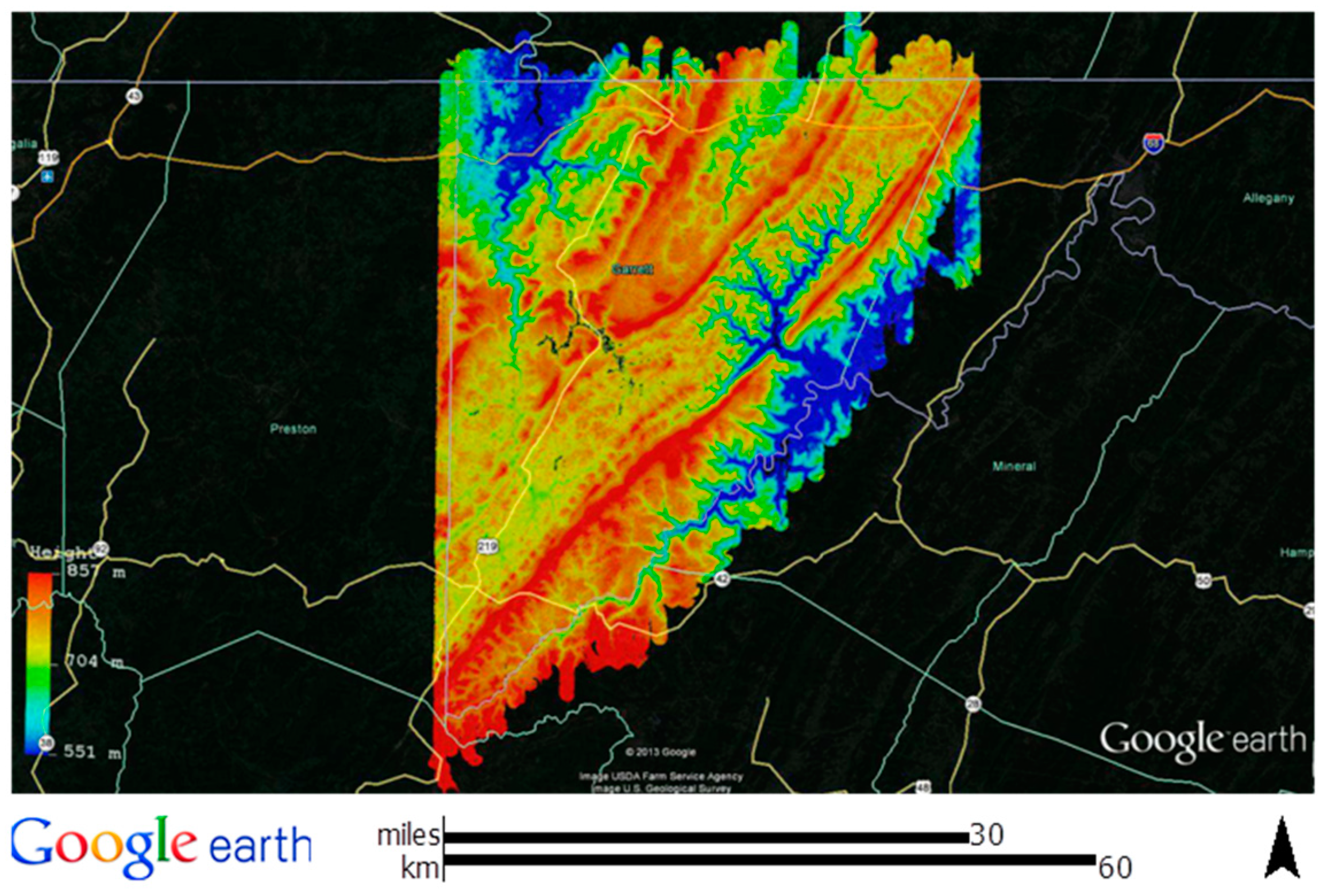
4.1. Garrett County, MD

Test flights of HRQLS have been funded by several interested customers to assess its capabilities for general surveying, tree height and biomass estimation, and bathymetry. For example, the University of Maryland, under a NASA grant, recently funded the airborne survey of Garrett County in Northwestern Maryland. The county—which is mountainous, heavily wooded, and has a total area of about 1700 km²—was surveyed in approximately 12 h of flight time, which included a 50% overlap of flight lines, four roundtrips from the host airport, and turns. Because of the low (10%) reflectance and density of the dominant green vegetation, HRQLS was operated from a nominal altitude of 2.29 km with a half-cone scanner angle of 17° (1.36 km swath) rather than the maximum value of 20° (1.62 km swath). At an aircraft velocity of 278 km/h, the resulting areal coverage was 378 km²/h. The full lidar data set for the county, color-coded from blue to red with increasing surface elevation, is shown superimposed on a Google Earth map of Garrett County in Figure 8. All flights were conducted during daylight hours.

One can get a sense of the surface spatial resolution by looking more closely at subsets of data within the map. Figure 9 provides different lidar views of a Garrett County coal mine. Details of the coal mining operation such as buildings, conveyor belts and coal piles can be clearly seen.

Figure 10 demonstrates the ability of the HRQLS-1 lidar to see through heavy forest canopy to the underlying surface and to distinguish between different canopy growth patterns [11].

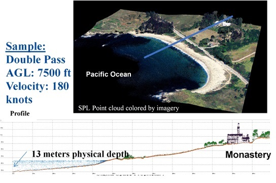
4.2. Monterey/Pt. Lobos, California

Another set of test flights was conducted in the vicinity of the Naval Post Graduate School in Monterey, California. Figure 11 provides a side-by-side view of the HRQLS-1 lidar data with a digital photograph of the same area. When the lidar data is fused with the digital imagery, one can generate color 3D images, as in Figure 12, or even fly-through movies of the area.

The Monterey flights also included topo-bathymetric experiments over the Pacific Ocean near Pt. Lobos. HRQLS-1, still operating at 2.3 km above the ocean surface to preserve the high speed contiguous mapping capability, was able to see the ocean bottom to an optical depth of roughly 18 m, as illustrated in Figure 13 This corresponds to an actual physical depth of about 13.5 m when one accounts for the refractive index of sea water. The low level of laser backscatter from the water and the large depth of penetration suggests very low turbidity. Water refraction effects have not been accounted for in the bottom image.

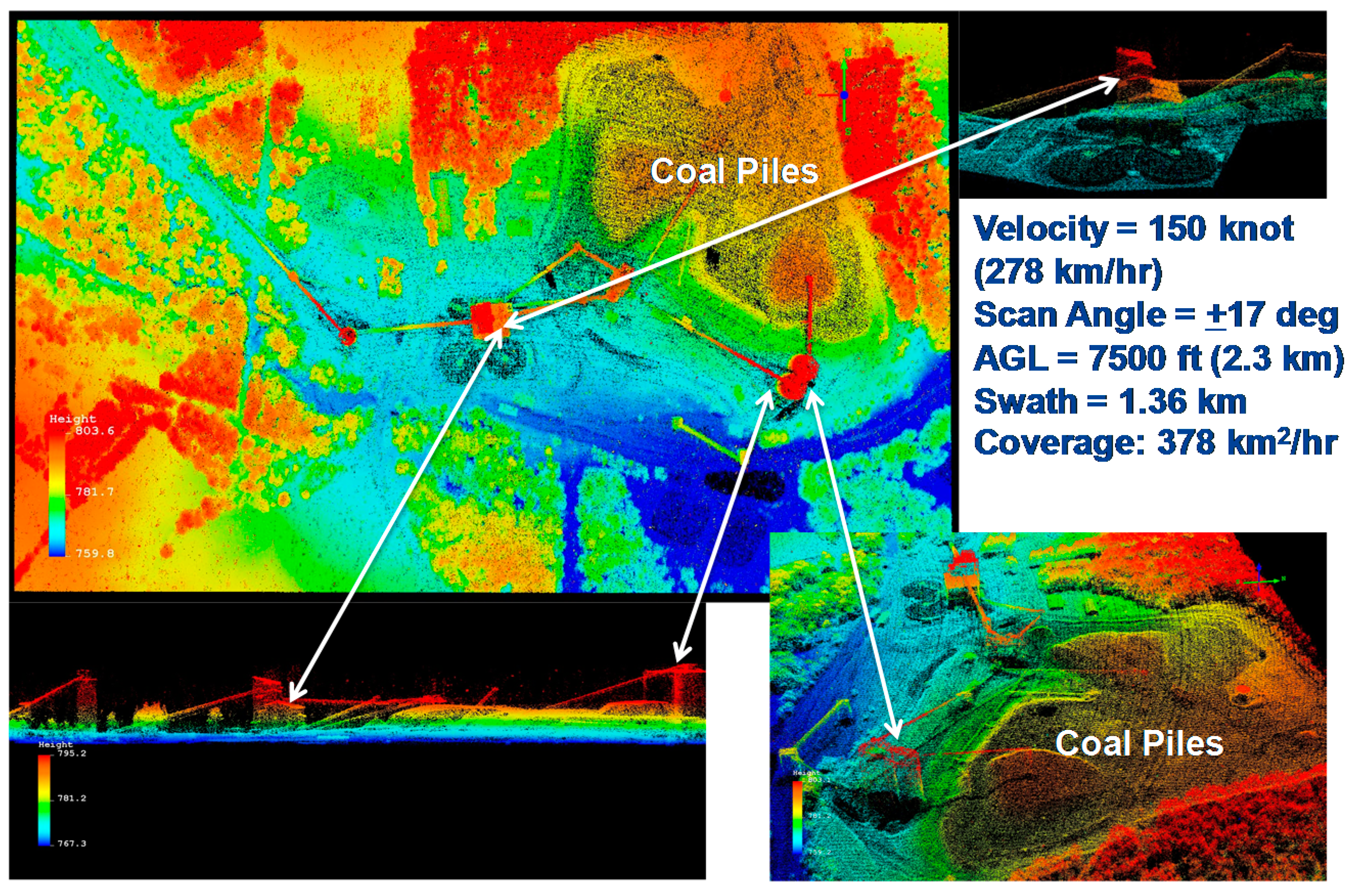
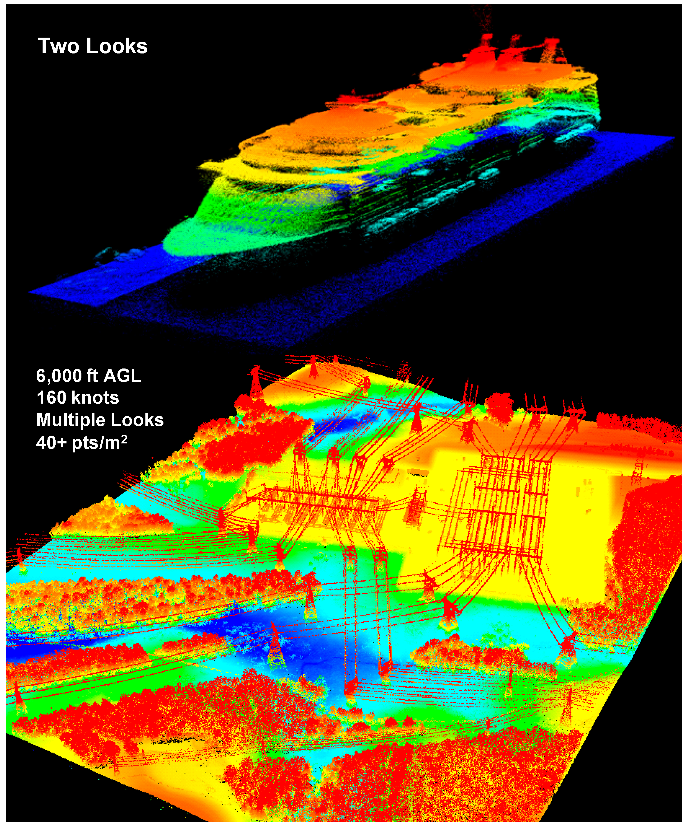
4.3. High Density Images

Two or more passes over the target area can produce extremely detailed images. In Figure 14, we show an image of a cruise ship docked at Ft. Lauderdale, FL which was obtained in only two HRQLS-1 passes and a multipass view of an electrical power line grid in North Carolina having a mean measurement density greater than 40 points per square meter.

5. Single Photon Lidar (SPL) vs. Geiger Mode (GM) Lidar

It should be mentioned that there is much interest within the lidar user community with regard to the characteristics and relative merits of the SPL systems described here vs. competing Geiger Mode Avalanche PhotoDiode (GMAPD) systems, which also utilize single photon detection. The earliest airborne GM lidar, Jigsaw, was developed with DARPA funding at the Massachusetts Institute of Technology/Lincoln Laboratories (MIT/LL) and was designed to image targets of military interest under tree canopies from low altitudes [12]. Later generations included the medium altitude Airborne Lidar Research Testbed (ALIRT), and the High Altitude Lidar Operations Experiment (HALOE) [13,14]. More recently, DARPA transferred GMAPD technology from MIT/LL to commercial entities, and Harris Corporation has introduced the first commercial GM system, The IntelliEarth™ Geospatial Solutions Geigermode Lidar Sensor [15].

5.1. Key Differences between SPL and GM Lidars

While both system types are capable of generating highly detailed 3D images, the following three bullets describe important differences between these two emerging single photon sensitive lidar technologies:

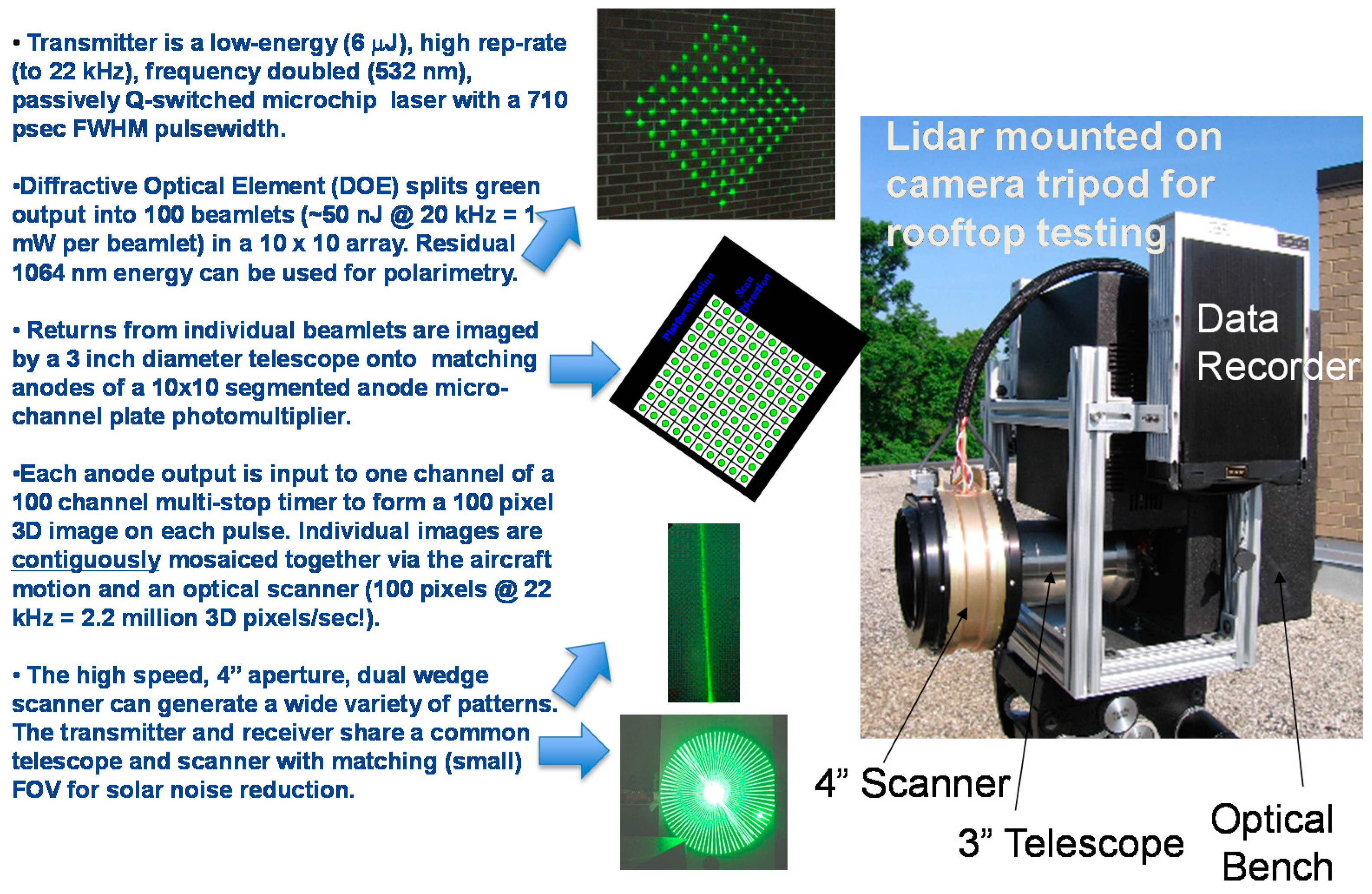
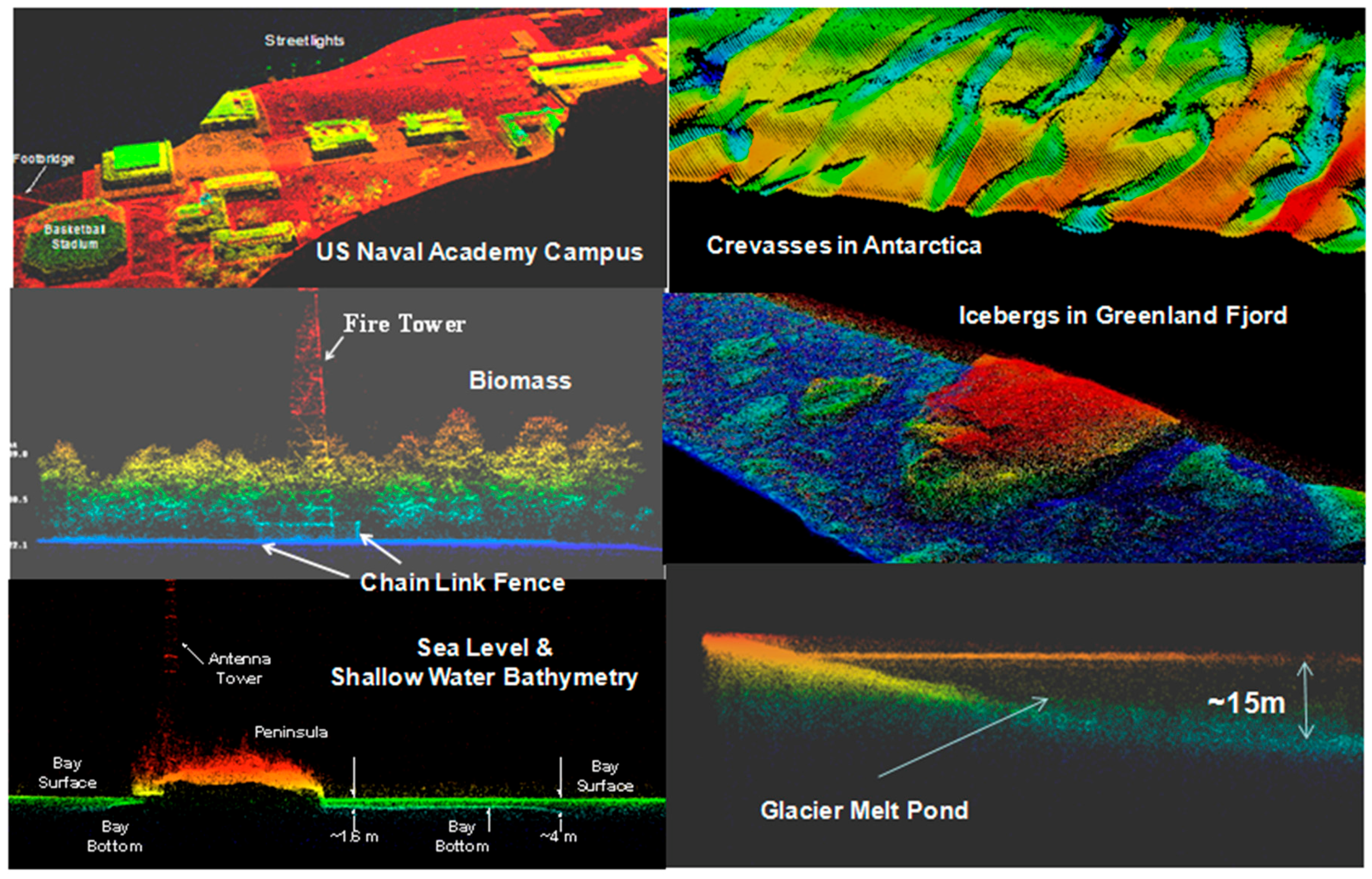
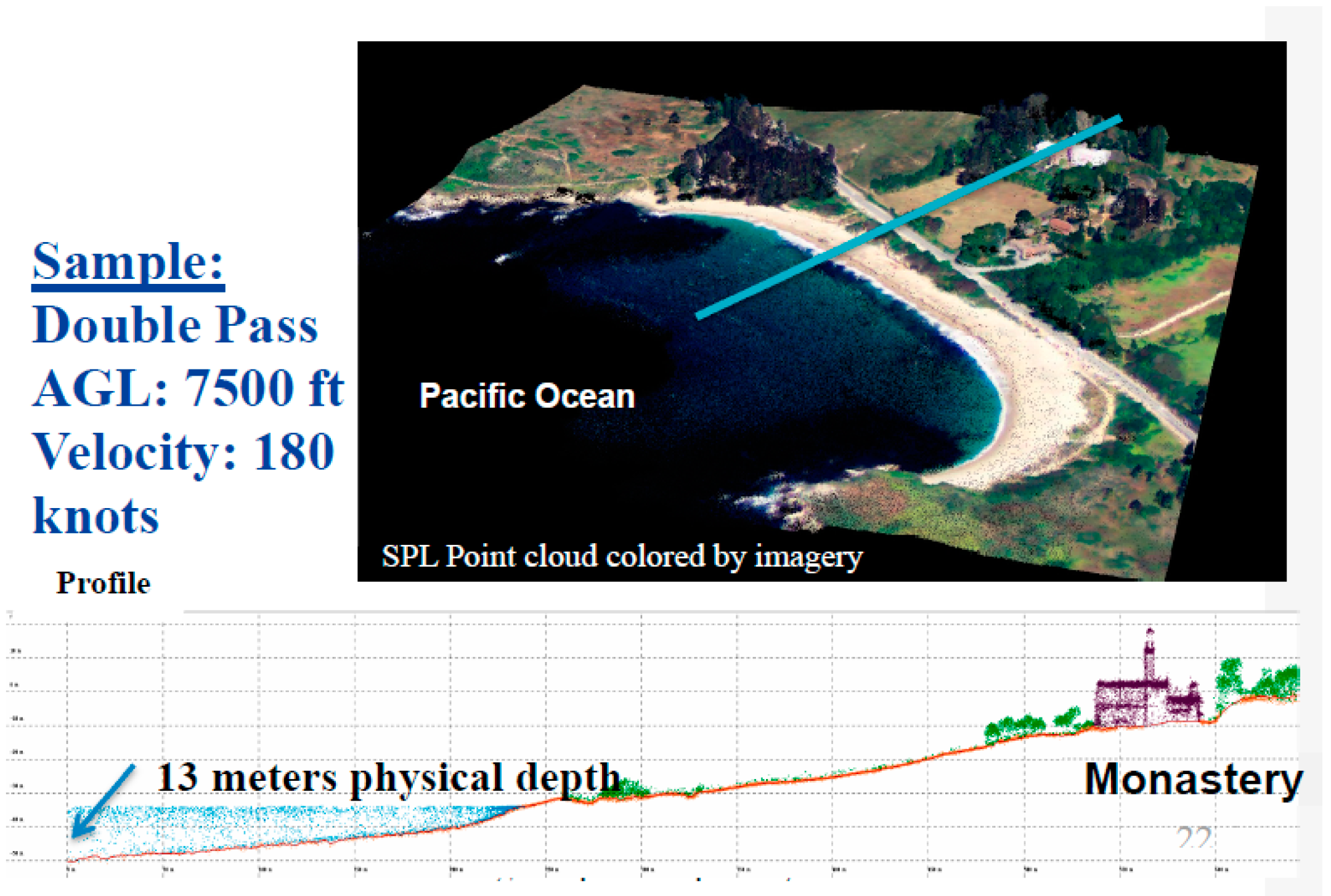
• Laser Wavelength: Current GM systems utilize the fundamental Nd:YAG wavelength at 1064 nm in the Near InfraRed (NIR) whereas Sigma SPLs use the frequency doubled green wavelength of Nd:YAG at 532 nm. The 1064 nm wavelength is sometimes touted as having several natural advantages including: (1) a factor of 3 lower solar background; (2) generally higher reflectances from natural surfaces such as soil/dry vegetation (25% vs. 15%) and green vegetation (65% vs. 10%); (3) slightly better atmospheric transmission; and (4) no frequency conversion losses in laser power which are typically on the order of 40% to 50% [2,15]. The 532 nm wavelength benefits from: (1) the availability of relatively mature and inexpensive, high efficiency array detectors and narrowband spectral filters; (2) detector dark count contributions to background noise are typically much lower in the visible spectrum; and (3) good transmission in water columns which allows solid land topography and bathymetry to be performed by a single instrument at a single wavelength as in Figure 13.
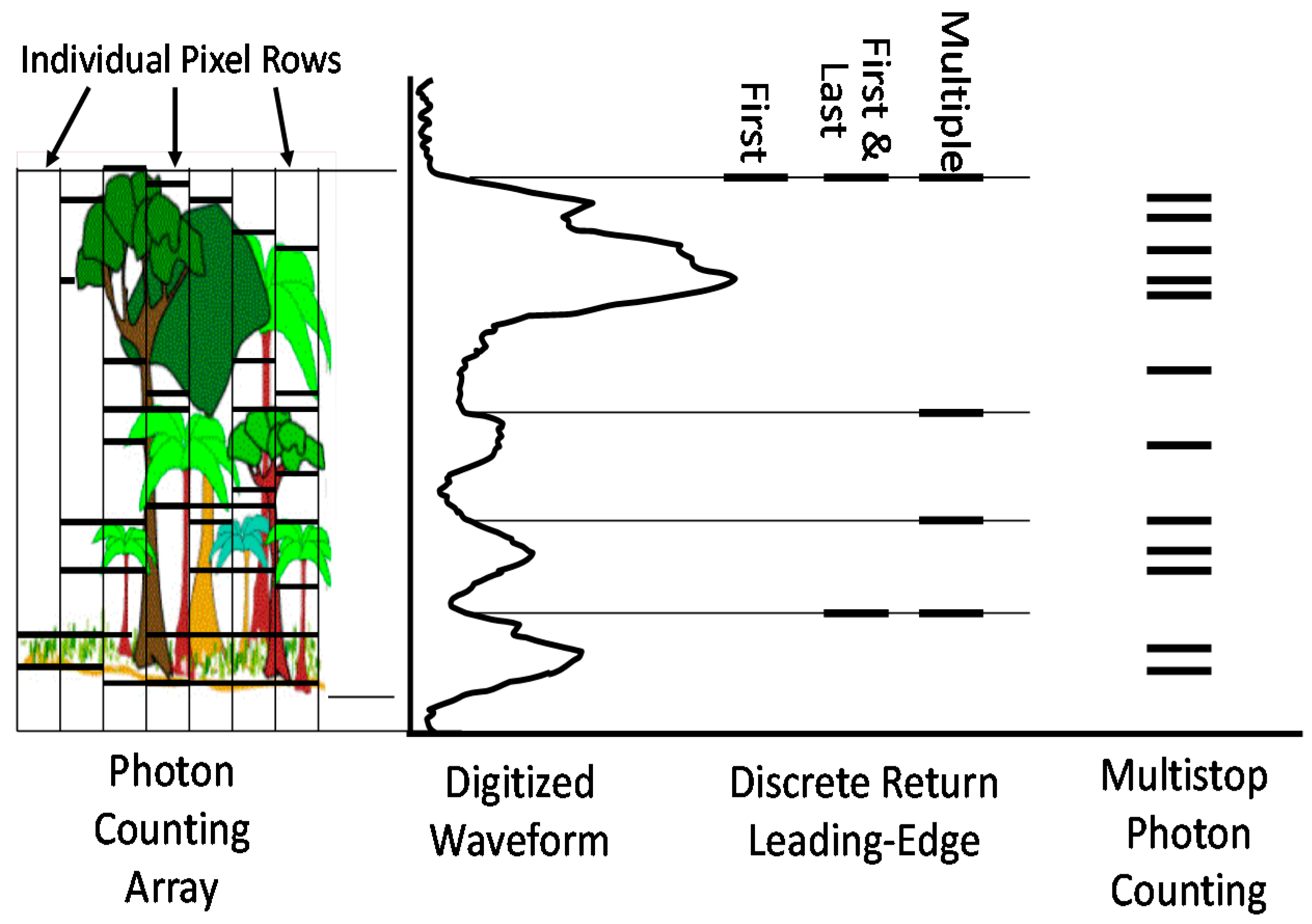
• Detector Array Size: Sigma SPLs use relatively inexpensive and compact COTS segmented anode microchannel plate photomultipliers which are currently available in 10 × 10 formats or 100 pixels per laser pulse. The Harris GM systems, on the other hand, currently utilize relatively expensive InP/InGaAsP SPAD 128 × 32 arrays/cameras containing 4096 pixels with on-chip readout rates in excess of 100 kHz [16]. In SPL systems, each pixel/anode essentially has a zero recovery time since each 1.6 mm × 1.6 mm pixel contains tens of thousands of microchannels, and therefore a single photon entering the photocathode activates a very small percentage of the available microchannels in the immediate vicinity of the photon strike. Thus, photons entering at slightly different spatial locations within the pixel experience the same amplification unless the microchannels become saturated, which generally has not been the case in field operations to date. In effect, a single SPL detector pixel behaves much like highly pixelated Geiger Mode array with the exception that all of the microchannel outputs are tied to a common anode and input to a common multistop timing channel capable of recording all of the photon events within the range gate and the pixel FOV. This limits the ground horizontal resolution to the FOV of the pixel which was 15 cm for Leafcutter and 50 cm square for the moderate to high altitude lidars. The current Sigma SPL receiver design typically accepts ten surface and/or noise events per pixel per pulse, but this is not a hard limitation. In effect, each SPL pixel acts as if it was a large array of individual GM SPADs covering the same FOV but tied to a common anode so that the timing of all photon events occurring within a given beamlet and pulse can be measured by a single, fast recovery, timing channel.
• Receiver Recovery Times: As just discussed, the SPL pixel recovery time of 1.6 nanoseconds (sometimes referred to as “deadtime” or “blanking loss” [15]) is limited not by the detector but by the timing receiver, whereas current GMAPD recovery times are typically in the range of 50 to 1600 nanoseconds depending on whether the Single Photon Avalanche Diodes (SPADs) making up the array are actively or passively quenched. This implies that SPLs can detect, within the same pixel, objects which are separated by only 0.24 m in range. In contrast, detected surfaces must be separated by 7.5 m or 240 m to be seen by an actively or passively quenched GMAPD respectively. Furthermore, each GMAPD in the array, as currently implemented in the Harris system, has only one measurement opportunity per imaging cycle although Harris claims that future asynchronous readout integrated circuits (ROICs) will enable multiple Time of Flight (TOF) measurements per APD per cycle [15]. While this would greatly enhance GM lidar performance, the detection rates within the small FOV of a given APD will still be limited by the longer quenching times.

We will now examine the impact of GMAPD recovery times for two very different daytime mapping scenarios, i.e., one in which the path between the aircraft and the solid target surface is unobstructed and one in which the target is obscured by a semi-porous obscurant (such as a tree canopy or ground fog). Night operations are not an issue for GMAPD lidars.

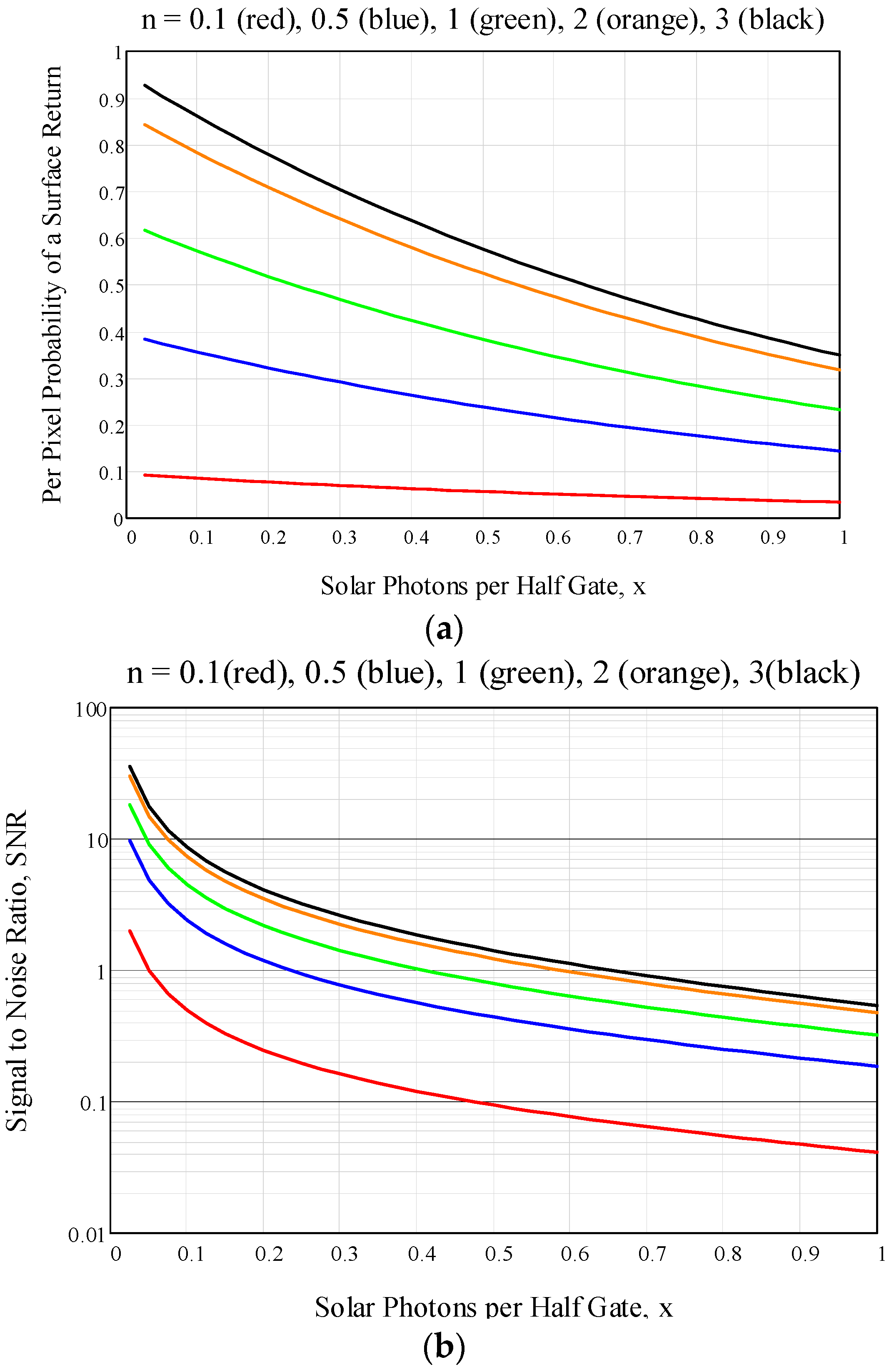
5.2. Mapping Unobstructed Solid Surfaces in the Presence of Solar Noise

A theoretical model for the solar background rate, Λ, is given in [2]

$$\mathsf{\Lambda }=N_{\mathsf{\lambda }}^0\left(\mathsf{\Delta }\mathsf{\lambda }\right){\mathsf{\Omega }}_r\frac{{\mathsf{\eta }}_c{\mathsf{\eta }}_r{A}_r}{\mathsf{\pi }h\mathsf{\nu }}\left[\mathsf{\rho }{T}_0^{1+\sec {\mathsf{\theta }}_z}\cos \mathsf{\psi }+\frac{1-T_0^{1+\sec {\mathsf{\theta }}_z}}{4\left(1+\sec {\mathsf{\theta }}_z\right)}\right]=\frac{0.05{\mathsf{\delta }}^2}{{\mathrm{cm}}^2\mathsf{\mu }\sec }$$

(2)

where the first and second terms respectively correspond to the background rates due to scattered solar radiation from the surface under study and the intervening atmosphere respectively. In obtaining the numerical value, we have ignored the atmospheric contribution and used numerical values pertinent to the Harris GM lidar [17]. The quantity $N_{\lambda }^0$ = 0.67 W/m²/nm is the extraterrestrial solar irradiance impinging on the Earth’s atmosphere at 1064 nm, Δλ = 3 nm is the width of the best spectral bandpass filter at 1064 nm based on a short web search, Ω = (δ/R)² is the solid angle viewed by a single GMAPD where R = 7.62 km is the range to the target and δ is the ground resolution, η_c = 0.3 is the Photon Detection Efficiency (PDE) of the detector, η_r = 0.75 is an estimated optical throughput efficiency of the receiver optics, A_r = 0.057 m² is the area of the Harris receive telescope, ρ = 0.65 is the surface reflectance of green vegetation at the laser wavelength, hν = 1.87 × 10⁻¹⁹ J is the laser photon energy, T₀~0.9 is the one-way atmospheric transmission at nadir from the aircraft, θ_z = 0 deg is the worst case solar zenith angle, and ψ = 0 is the worst case subtended angle between the Sun and the surface normal.

In either system type (SPL or GM), the solar background counts during daylight operations can be substantially reduced by installing narrowband spectral filters and minimizing the range gate, the collecting area of the telescope and/or the pixel FOV. This is especially important for the single stop GM system, however, since a noise count occurring within the range gate prior to the surface return will result in the loss of that surface measurement for one full array mapping cycle.

For the SPL, a single timing event is generated by a solid surface, irregardless of the number of photons received, since the subnanosecond laser pulsewidth is short compared to the pixel recovery time of 1.6 ns. As a result, the amplitude of the SPL anode output will vary if the “simultaneous” surface returns are spread over multiple microchannels and summed within the pixel/anode. Single photon noise counts within the range window are recorded as separate random events displaced in range and time from the surface returns and later eliminated via noise editing algorithms described previously. Unlike individual GM/APDs, the detection of a solar photon in an SPL pixel does not prevent the pixel from detecting the surface.

For unobscured hard targets, the principal concern raised by the single stop limitation of current GM sensors is the impact of the solar background on the surface probability of detection which, in daylight operations, dominates other noise sources such as detector dark counts. There are only three possible outcomes for a given GM pixel per imaging cycle: (1) a surface photon is detected; (2) no photon is detected; or (3) a background count is detected. If the range gate is approximately centered on the surface and Λ is the solar count rate observed by a single APD, the probability of detecting the surface is given by

$$P_s(n,\mathsf{\Lambda }{\mathsf{\tau }}_g)=\exp \left(-\frac{\mathsf{\Lambda }{\mathsf{\tau }}_g}{2}\right)P_s=\exp \left(-\frac{\mathsf{\Lambda }{\mathsf{\tau }}_g}{2}\right)\left[1-\exp (-n)\right]$$

(3)

where the first term is the probability that the APD is not triggered by solar noise in the first half of the gate, and the second term is the Poisson probability that the surface return, consisting of n detected photoelectrons, is detected by a receiver with a single photon threshold. Similarly, the probability that zero counts are detected is given by

$$P_z(n,\mathsf{\Lambda }{\mathsf{\tau }}_g)=\exp \left(-\frac{\mathsf{\Lambda }{\mathsf{\tau }}_g}{2}\right)\left[1-Ps(n,\mathsf{\Lambda }{\mathsf{\tau }}_g)\right]\exp \left(-\frac{\mathsf{\Lambda }{\mathsf{\tau }}_g}{2}\right)=\exp (-\mathsf{\Lambda }{\mathsf{\tau }}_g)\exp (-n)$$

(4)

and, since the three probabilities must sum to 1, the probability that a solar background count is detected is given by

$$P_b(n,\mathsf{\Lambda }{\tau }_g)=1-P_s(n,\mathsf{\Lambda }{\tau }_g)-P_z(n,\mathsf{\Lambda }{\tau }_g)=\left[1-\exp \left(-\frac{\mathsf{\Lambda }{\tau }_g}{2}\right)\right]\left[1+\exp \left(-\frac{\mathsf{\Lambda }{\tau }_g}{2}\right)\exp (-n)\right]$$

(5)

The ratio of signal counts to solar counts is obtained by dividing (3) by (5) to yield

$$SNR=\frac{P_s(n,\mathsf{\Lambda }{\tau }_g)}{P_b(n,\mathsf{\Lambda }{\tau }_g)}=\frac{1-\exp (-n)}{\left[\exp \left(\frac{\mathsf{\Lambda }{\tau }_g}{2}\right)-1\right]\left[\left[1+\exp \left(-\frac{\mathsf{\Lambda }{\tau }_g}{2}\right)\exp (-n)\right]\right]}$$

(6)

Figure 15a shows plots of Equation (3) for the fraction of GMAPDs recording surface returns over a range of surface signal strengths, n = 0.1 to 3, and the mean number of noise photons occurring in the first half of the range gate, x = Λτ_g/2 = 0 to 1. Figure 15b, plotting Equation (6), shows the ratio of signal to noise counts versus the same parameters. It is worthwhile to note that achieving even the lowest value of n = 0.1 in all 4096 pixels (one detected surface photon per APD in 10 pulses) would require a total signal strength of 410 photoelectrons (pe) detected across the array. This is comparable to what many Digitizer Waveform lidars require and what the HAL lidar achieves from similar AGLs for ground reflectances of 15%, or higher, i.e., 4 pe per pixel over 100 pixels, but the per pixel probability of detection is close to 100% as compared to 10% or less as in Figure 15a. Nevertheless, the GM lidar has the potential of recording surface returns from 4 times as many pixels provided the solar noise counts can be adequately suppressed.

The plots in Figure 15a would suggest that we strive for a value of

$$x\equiv \frac{\mathsf{\Lambda }{\mathsf{\tau }}_g}{2}=\frac{0.05{\mathsf{\delta }}^2{\mathsf{\tau }}_g}{2{\mathrm{cm}}^2\mathsf{\mu }\sec }<0.2$$

(7)

in order to avoid severely diminishing the probability of detecting a surface return. A typical range gate in our high altitude flights is τ_g = 5 μs, which, from (7), would suggest a pixel dimension at the ground of δ < 1.3 cm or a maximum array area FOV at the ground of AGM = 4096 (1.3 cm)² = 0.7 m². The latter area is 36 times smaller than the HAL area for a single pulse and, while a 1.3 cm horizontal spatial resolution would be outstanding, the effect on the rate of areal coverage would not.

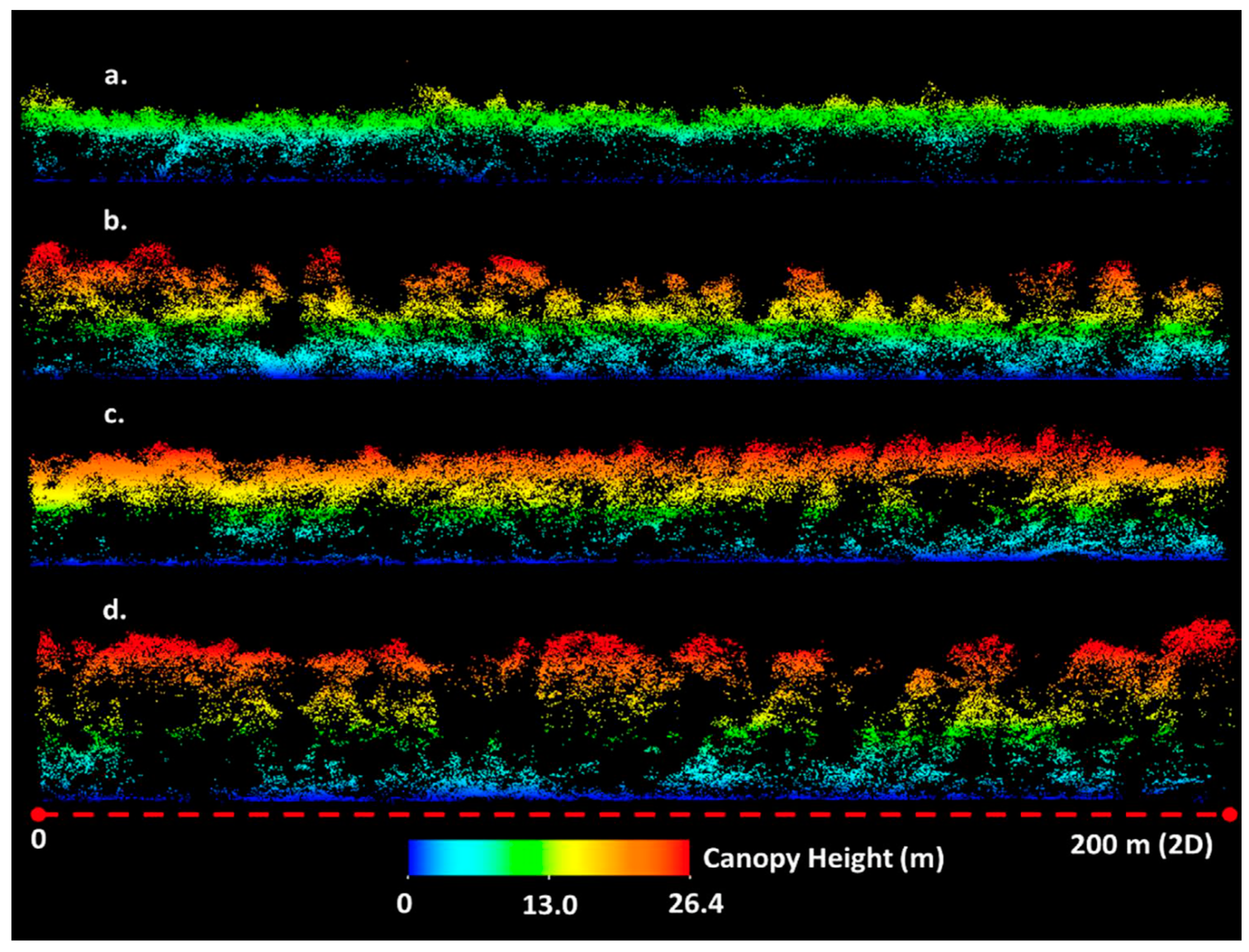
5.3. Viewing the Surface through Semi-Porous Obscurants Such as Tree Canopies

It has long been known from early experiments conducted with the Jigsaw GM system at MIT/LL that, in order to detect military vehicles under dense tree canopies, one had to reduce the pulse energy per pixel in order to reduce the probability that a photon from the canopy would disable the pixel and prevent observation of the surface under the canopy. Therefore, since the tree elements (leaves, branches, etc.) are opaque to laser light, a recognizable surface image could only be generated by making many low energy measurements from a wide variety of aspect angles in order to take advantage of any existing canopy “holes” between the aircraft and the surface. This can be mathematically represented by multiplying the probability of detecting the surface by the probability that the measurement is not disabled by a photon reflected off a tree element. From Poisson statistics, the probability of detecting a target beneath a canopy (or fog bank) with one-way transmission T_c is given by

$$PD(n_s,\gamma )=\exp \left[-\frac{\gamma n_s}{2}\left(1-T_c^2\right)\right]\left[1-\exp \left(-T_c^2{n}_s\right)\right]$$

(8)

where n_s is the expected number of detected photoelectrons from the unobscured target,

$$\mathsf{\gamma }=\frac{{\mathsf{\rho }}_c}{{\mathsf{\rho }}_t}$$

(9)

and ρ_c and ρ_t are the reflectances of the canopy and target respectively. The second term in the equation gives the probability of detecting the surface signal with a single photon sensitive receiver while the first term gives the probability of disabling the receiver due to the detection of a canopy return. As mentioned previously, the Sigma SPL detector/receiver has a very short recovery time on the order of 1.6 ns and therefore only the second term in the equation is relevant. Figure 16 shows the surface detection probability for a tree canopy with a one way transmission T_c = 0.4 as a function of the unobscured signal strength (T_c = 1). The black curve in the plot shows the probability of detecting the unobscured target vs. the mean signal strength expressed in detected photoelectrons. The red curve gives the same probability for a low deadtime single photon sensitive receiver in the presence of a tree canopy with a one-way transmission of T_c = 0.4 (T_c² = 0.16). The remaining three curves show the Geiger Mode probabilities for different values of γ. Note that, for each value of γ, there is an optimum unobscured signal strength for detecting the underlying surface in qualitative agreement with the early Jigsaw experiments. In all cases, the peak Geiger Mode detection probabilities fall substantially below the SPL values, especially when the canopy has a higher reflectance than the final target (γ > 1). The 6.5 times stronger reflectance of vegetation at 1064 nm vs. 532 nm (65% vs. 10%) mentioned in Bullet 1 of Subsection 5.1 increases the value of γ substantially and further reduces the probability of seeing the under-canopy surface. In addition, the higher tree reflectance creates a 6.5/3 = 2.2 times stronger solar background during daylight operations which was not included in the plots of Figure 16 and Figure 17.

The theoretical performance of SPL and GM lidars over a wide range of one-way tree canopy transmissions (T_c = 0.1 to 1) is provided by Figure 17. The reduction in canopy transmission could be due to more dense foliage or a longer slant range through a canopy with higher one-way transmission when viewed from nadir. This is an important consideration since the key to under canopy observations is finding “all the available” holes”. The curves in the top left of the figure demonstrate how the GM probability of detecting the surface falls as the one-way canopy transmission decreases due to the fact that the lidar cannot “power” its way through the canopy by increasing the unobscured signal strength because of the one return per APD limitation. The curves in the bottom right of the figure show the relative surface detection rate of the SPL and GM systems for the same range of tree canopy transmissions where the SPL can, in fact, “power” its way through the canopy as in Figure 16.

5.4. Brief Summary of the Theoretical Results

While there are clearly no issues with night operations of GM lidars as indicated by a large number of highly detailed 3D images posted on the Harris web site [17], the present analysis suggests that the expected solar noise over high reflectance surfaces, such as green vegetation (ρ = 0.65) could greatly reduce the PDE of individual GMAPD pixels having reasonably sized FOVs. This in turn would greatly reduce the rate at which large areas can be mapped in daylight. It must be mentioned, however, that Harris Corporation strongly claims an acceptable daylight capability on their web site [17] and a limited amount of daytime data was included in a recent USGS study [18]. Furthermore, the current analysis indicates that GM lidars would appear to be far inferior to SPLs when probing dense tree canopies.

6. Summary

Imaging SPLs operating at the 532 nm wavelength can provide seamless topographic and bathymetric maps from a single instrument. Single photon sensitivity allows a moderate power laser beam to be split, by a passive holographic element, into a 10 × 10 array of individual beamlets, whose images in the receiver plane fall onto a matching array of single photon sensitive, high bandwidth pixels. In addition to increasing the surface measurement rate to several megapixels per second for subnanosecond pulse lasers operating in the tens of kHz range, the arrays allow contiguous, decimeter resolution, alongtrack and crosstrack mapping of the surface on a single overflight with modest telescope and scanner apertures (7.5 cm to 15 cm) and scanner speeds on the order of 20 Hz (1200 RPM). Higher transverse spatial resolutions can be achieved by reducing the swath width or by making multiple overlapping passes over the site. The fast recovery times (1.6 ns) of the pixels and their individual timing channels provide a multistop capability that allows the SPLs to operate effectively under conditions of strong solar illumination and to penetrate semiporous obscurants such as tree canopies, ground fog, etc. The SPLSs are designed to have per pixel probabilities of detection on the order of 95% for a 10% reflectance surface (mean of 3 pe per pixel from green vegetation) and greater than 99% for reflectances greater than 15% (mean of 4 pe per pixel from soil or dry vegetation). Thus, the mean 300 photoelectron returns from a tree canopy over the full array is comparable to that of some conventional Digitized Waveform lidars but with the added advantage that the location of the scattering source within the canopy is identified in all three dimensions as opposed to being lumped together into a single dimension, range, thereby resulting in a more realistic image of the canopy.

As the SPLs have progressed to higher operational altitudes in order to provide wider swaths and faster areal coverage, we have had to address new technical challenges such as the availability of COTS laser/telescope/detector combinations to meet the higher link demands. Table 1 in Section 2.7 provides a summary of the key subsystem parameters for the various SPLs flown to date. Solar background has been minimized through the use of a 0.3 nm FWHM spectral filter and a small pixel Field of View, typically defined by a 50 cm × 50 cm square on the ground. The vast majority of the detected noise is eliminated via noise editing algorithms as described in Section 3. Also, at the higher AGLs, a corrector wedge is added to the common transmit/receive optical scanner to reimage the transmit beamlet array onto the detector array at the nominal AGL and scan speed. For alternative AGLs, the scan speed must be adjusted from its nominal value to achieve maximum overlap of the transmit and receive FOVs. In addition, angular biases, as well as atmospheric refraction and pulse group velocity effects, play a bigger role in achieving the necessary geolocation accuracy due to the longer slant range distances. As a result, we have developed algorithms and software to find and eliminate biases based on multiple looks at distinct features in the overall point cloud such as the corners of buildings.

Lidar users in the mapping community are most concerned about geolocation errors and spatial resolution. Geolocation is assessed by comparing lidar elevation products to surveyed ground control points. The HAL system was flown over a 400 square kilometer area at an AGL of approximately 7.6 km. A total of 22 ground points were surveyed and compared to elevations derived from the point cloud. After removing bias, an elevation RMS of 9 cm, meeting the highest USGS QL-1 requirement of 10 cm, was obtained [8]. In an earlier flight experiment over Monterey CA, HRQLS-1 point cloud results were compared to 21 points measured to 3 cm vertical accuracy by the Naval Postgraduate School and resulted in a similar 9.3 cm RMS Standard deviation. In addition, both HAL and HRQLS-1 easily meet the USGS QL-1 requirements on measurement point densities (>8 pts/m²).

In 2015, Sigma’s HRQLS-1 SPL and Harris GM systems participated in a series of USGS-sponsored field trials in the state of Connecticut in which the point clouds were analyzed by two independent and highly experienced lidar analysis groups (Woolpert and Dewberry) and presented at the International Laser Mapping Forum (ILMF2016) in Denver, Colorado. For recent field evaluations of the HRQLS-1 SPL and/or the Harris GM system over a wide variety of terrain types and opinions on their future operational role with respect to conventional linear mode lidars, the reader is referred to the following papers [19,20,21]. The current SPL and GM lidars are generally viewed as being highly competitive with conventional lidars when it comes to large scale mapping missions over unobscured terrain. On the other hand, as discussed in Section 5, the fast pixel recovery times would appear to give the SPL approach a significant advantage over GM systems for daytime mapping missions requiring wide range gates and/or the penetration of semi-porous obscurants such as tree canopies, ground fog, etc. As mentioned previously, use of the green wavelength also permits topo-bathymetric measurements to be carried out by a single, compact SPL instrument. Our newest moderate altitude SPL, HRQLS-2, and presumably the latest version of the Harris Corporation GM lidar, are expected to participate in a second set of USGS-sponsored experiments to be carried out over large areas in South Dakota in late 2016.

Commercial users of conventional lidars also ask whether or not SPLs can generate intensity information. In principle, aggregated single photon returns collected over a sufficient surface area could be used to ascertain reflectance but our SPL systems are designed to collect as many surface measurements as possible per square meter by multiphoton surface returns. This provides little discrimination between different surface reflectances since all surfaces over 10% reflectance provide 95 to 100 pixel returns per pulse. However, one Sigma colleague has developed an as yet unpublished but highly successful procedure applicable to daytime operations [22] while a second is experimenting with a second hardware approach applicable to both day and night missions [23].

In preparation for 3D imaging that can be viewed by the aircraft crew or transmitted to a ground station in near real time, we are currently implementing inflight algorithms and onboard processors that edit out solar and/or electronic noise and correct for atmospheric effects. Furthermore, analyses conducted for NASA have shown that the scanning SPL technique can even be extended to orbital altitudes for the globally contiguous mapping of extraterrestrial planets and moons [2,4,16] using space-qualified transmitters and timing receivers being developed for NASA’s ATLAS SPL lidar on the ICESat-2 mission scheduled to be launched in 2017 [9]. For example, the three moons of Jupiter of most interest to NASA can each be globally mapped with 5 m horizontal resolution and decimeter vertical resolution in as little as two months for the larger moons, Ganymede and Callisto, and one month for Europa [24].

References

1. Degnan, J.; McGarry, J.; Zagwodzki, T.; Dabney, P.; Geiger, J.; Chabot, R.; Steggerda, C.; Marzouk, J.; Chu, A. Design and performance of an airborne multikilohertz, photon-counting microlaser altimeter. Int. Arch. Photogramm. Remote Sens. 2001, XXXIV-3/W4, 9–16. [Google Scholar]
2. Degnan, J. Photon-Counting Multikilohertz Microlaser Altimeters for Airborne and Spaceborne Topographic Measurements. J. Geodyn. 2002, 4, 503–549. [Google Scholar] [CrossRef]
3. Harding, D. Pulsed Laser Altimeter Ranging Techniques and Implications for Terrain Mapping. In Topographic Laser Ranging and Scanning: Principles and Processing; Shan, J., Toth, C.K., Eds.; CRC Press: Boca Raton, FL, USA, 2009. [Google Scholar]
4. Degnan, J.; Wells, D.; Machan, R.; Leventhal, E. Second Generation 3D Imaging Lidars based on Photon-Counting. In Proceedings of SPIE Optics East, Boston, MA, USA, 12 September 2007.
5. Carter, W.; Shrestha, R.; Slatton, K. Photon counting airborne laser swath mapping (PC-ALSM). In Gravity, Geoid, and Space Missions; Jekeli, C., Bastos, L., Fernandez, J., Eds.; Springer: Berlin/Heidelberg, Germany, 2004; pp. 214–217. [Google Scholar]
6. Cossio, T.; Slatton, C.; Carter, W.; Shrestha, K.; Harding, D. Predicting topographic and bathymetric measurement performance for low-SNR airborne lidar. IEEE Trans. Geosci. Remote Sens. 2009, 47, 2298–2315. [Google Scholar] [CrossRef]
7. Degnan, J.J. A Conceptual Design for a Spaceborne 3D Imaging Lidar. E&I Electrotechnik und Informationstechnik (Austria) 2002, 4, 99–106. [Google Scholar]
8. Gluckman, J. Design of the processing chain for a high-altitude, airborne, single photon lidar mapping instrument. Proc. SPIE 2016. [Google Scholar] [CrossRef]
9. Abdalati, W.; Zwally, H.; Bindschadler, R.; Csatho, B.; Farrell, S.; Fricker, H.; Harding, D.; Kwok, R.; Lefsky, M.; Markus, T.; et al. The ICESat-2 laser altimetry mission. Proc. IEEE 2010, 98, 735–751. [Google Scholar] [CrossRef]
10. McGill, M.; Markus, T.; Scott, V.S.; Neumann, T. The Multiple Altimeter Beam Experimental Lidar (MABEL): An Airborne Simulator for the ICESat-2 Mission. J. Atmos. Ocean. Technol. 2013, 30, 345–352. [Google Scholar] [CrossRef]
11. Swatantran, A.; Tang, H.; Barrett, T.; DeCola, P.; Dubayah, R. Rapid, High-Resolution Forest Structure and Terrain Mapping over Large Areas using Single Photon Lidar. Sci. Rep. 2016. [Google Scholar] [CrossRef] [PubMed]
12. Vaidyanathan, M.; Blask, S.; Higgins, T.; Clifton, W.; Davidsohn, D.; Carson, R.; Reynolds, V.; Pfannenstiel, J.; Cannata, R.; Marino, R.; et al. JIGSAW Phase III: A miniaturized airborne 3-D imaging laser radar with photon-counting sensitivity for foliage penetration. Proc. SPIE 2007. [Google Scholar] [CrossRef]
13. Knowlton, R. Airborne Ladar Imaging Testbed; Tech Notes; MIT Lincoln Laboratory: Lexington, MA, USA, 2011; Available online: http://www.princetonlightwave.com/products/geiger-mode-cameras/ (accessed on 17 November 2016).
14. Gray, G. High Altitude Lidar Operations Experiment (HALOE)—Part 1, System Design and Operation. In Proceedings of the Military Sensing Symposium, Active Electro-Optic Systems, Paper AH03, San Diego, CA, USA, 12–14 September 2011.
15. Clifton, W.; Steele, B.; Nelson, G.; Truscott, A.; Itzler, M.; Entwhistle, M. Medium altitude airborne Geiger-mode mapping Lidar system. Proc. SPIE 2015, 9465, 946506. [Google Scholar] [CrossRef]
16. Falcon IR Camera. Available online: http://www.princetonlightwave.com/products/geiger-mode-cameras/ (accessed on 17 November 2016).
17. Harris Corporation. Available online: http://www.apsg.info/resources/Documents/Presentations/APSG34/IntelliEarth_Presentation_APSG34_Oct_2015.pdf (accessed on 14 November 2016).
18. Higgins, S. Single Photon and Geiger Mode vs. Linear Mode Lidar. SPAR 3D. 2016. Available online: http://www.spar3d.com/news/lidar/single-photon-and-geiger-mode-vs-linear-mode-lidar/ (accessed on 14 November 2016).
19. Li, Q.; Degnan, J.; Barrett, T.; Shan, J. First Evaluation on Single Photon-Sensitive Lidar Data. Photogramm. Eng. Remote Sens. 2016, 82, 455–463. [Google Scholar] [CrossRef]
20. Abdullah, Q. A Star is Born: The State of New Lidar Technologies. Photogramm. Eng. Remote Sens. 2016, 82, 307–312. [Google Scholar] [CrossRef]
21. Higgins, S. Single Photon Lidar Proven for Forest Mapping. SPAR 3D. 2016. Available online: http://www.spar3d.com/news/lidar/single-photon-lidar-proven-forest-mapping/ (accessed on 14 November 2016).
22. Field, C. Sigma Space Corporation, Lanham, MD, USA. Private communication, 2014. [Google Scholar]
23. Machan, R. Sigma Space Corporation, Lanham, MD, USA. Private communication, 2016. [Google Scholar]
24. Degnan, J. Rapid, Globally Contiguous, High Resolution 3D Topographic Mapping of Planetary Moons Using a Scanning, Photon-Counting Lidar. International Workshop on Instrumentation for Planetary Missions, GSFC. 2012. Available online: http://www.lpi.usra.edu/meetings/ipm2012/pdf/1086.pdf (accessed on 14 November 2016).
Figure 1. A comparison of Single Photon Lidars with conventional Discrete Return and Digitized Waveform lidars in interacting with a tree canopy (Courtesy of D. Harding, NASA GSFC).
Remotesensing 08 00958 g001
Figure 2. Leafcutter was the first Sigma Single Photon Lidar (SPL) to split the laser beam into 100 beamlets. In early mapping missions, the dual wedge scanner was used to generate either linear raster scans at 45° to the flight line or a conical scan with cone half angles up to 13.5 degrees. At the design AGL of 1 km, pixels on the ground were separated by 15 cm. Contiguous alongtrack and crosstrack mapping on a single pass was achieved by ensuring: (1) that the distance traveled by the aircraft during one scan cycle did not exceed the 1.5 m dimension of the single pulse array; and (2) that ground array patterns from subsequent pulses overlapped along the full circumference of the conical scan and the length of the linear scans.
Remotesensing 08 00958 g002
Figure 3. A collage of daytime images created on a single overflight by the Leafcutter SPL. The images in the left half were over low reflectance (10% to 15%) surfaces at above ground levels (AGLs) of 1 km or less while those in the right half were high reflectance cryospheric measurements in Greenland and Antarctica from AGLs up to 2.5 km. The images are color-coded according to the lidar-derived surface elevation (blue = low, red = high). Note the bathymetry results in the bottom two images.
Remotesensing 08 00958 g003
Figure 4. NASA Mini-ATM (Airborne Topographic Mapper) and its designated host aircraft, the Viking 300 micro-UAV.
Remotesensing 08 00958 g004
Figure 5. Moderate altitude HRQLS-1 and HRQLS-2 lidars and the King Air B200 host aircraft.
Remotesensing 08 00958 g005
Figure 6. The NASA MABEL pushbroom lidar, jointly developed by NASA Goddard Space Flight Center and Sigma Space Corporation, has successfully generated 2D surface profiles in Greenland from an AGL of 20 km. The surface returns are highly spatially correlated and stand out against the dense “salt-and-pepper” solar noise background resulting from the high reflectance (typically 80% to 96%) of snow and ice at 532 nm.
Remotesensing 08 00958 g006
Figure 7. The automated filtering of HRQLS-1 lidar data taken on a single overflight of a residential community in Oakland, MD. The raw/unfiltered point cloud data is taken with a range gate of 4.6 microseconds corresponding to a total range interval of 690 m. The color scheme is deep blue to red in order of increasing elevation, and it should be mentioned that the solar noise is equally dense below the surface but does not show up as well in the raw unfiltered image because of the poor contrast against the black background. The first stage filter isolates a 90 m interval that contains the surface data as well as roughly 13% of the total noise, and the second stage filter uses narrower range bins (~5 m) to eliminate the vast majority of the remaining noise.
Remotesensing 08 00958 g007
Figure 8. This color-coded elevation map of Garrett County, occupying approximately 1700 km2 in the state of Maryland, was generated by HRQLS-1 from an AGL of 2.3 km. Total flight duration was approximately 12 h at an air speed of 278 km/h which included a 50% overlap between flight line, ferries, and turn maneuvers. The scanner was operating with a cone half angle of 17° resulting in a swath of 1.36 km and a mapping rate of 378 km2/h. Highest and lowest elevations are: red = 857 m, blue = 551 m.
Remotesensing 08 00958 g008
Figure 9. A Garrett County coal mine in which buildings, conveyor belts, and even black coal piles are clearly visible. Elevation Scales: Top Left red = 803.4 m, blue = 759.8 m; Bottom Left and Bottom Right red = 795.2 m, blue = 767.3 m.
Remotesensing 08 00958 g009
Figure 10. HRQLS-1 SPL point cloud profiles showing different growth patterns within a 1 square kilometer of forested area in Garrett County, MD. (a) Short even aged stand with little understory vegetation; (b) Uneven aged stand composed of tall trees and dense midstory vegetation; (c) Even aged stand with some mid and understory growth; (d) Tall open stand with distinct understory vegetation (Courtesy of the University of Maryland [11]).
Remotesensing 08 00958 g010
Figure 11. HRQLS-1 lidar image and digital color photograph of the area surrounding the Naval Post Graduate School in Monterey, California.
Remotesensing 08 00958 g011
Figure 12. “Fused” HRQLS-1 lidar-photographic 3D image of the Naval Post Graduate School in Monterrey, California.
Remotesensing 08 00958 g012
Figure 13. Top: Colored HRQLS-1 lidar topo-bathymetric 3D pointcloud of a hilltop monastery and the beach at Pt. Lobos near Monterey, CA; Bottom: The bottom image shows the 2D lidar profile along the blue line in the top figure and extending from the monastery to the beach and into the Pacific Ocean to an optical depth of 17.3 m or a physical depth of 13 m. Vertical grid size = 10 m, Horizontal grid size = 50 m.
Remotesensing 08 00958 g013
Figure 14. Top: Two passes of HRQLS-1 over a cruise ship docked at Ft. Lauderdale, Florida; Bottom: Multiple HRQLS-1 passes over a power line grid in North Carolina yielding over 40 points per square meter from an AGL of 1.83 km and an aircraft velocity of 296 km/h.
Remotesensing 08 00958 g014
Figure 15. (a) Fraction of pixels recording surface returns as a function of surface signal strength, n, and mean number of noise photons detected within a half range gate; (b) ratio of signal to noise counts as a function of the same two parameters.
Remotesensing 08 00958 g015
Figure 16. Surface detection probabilities for SPL and Geiger Mode (GM) lidars as a function of the unobscured signal strength for a tree canopy having a one way transmission of 40%. Unlike the GM lidar which has an unobscured signal strength that optimizes the surface detection probability, the SPL lidar can “power” through the canopy by increasing the laser pulse energy.
Remotesensing 08 00958 g016
Figure 17. The relative performance of SPL and GM lidars over a wide range of one-way tree canopy transmissions (Tc = 0.1 to 1) A value γ = 1 is assumed. The top left graph demonstrates that, as the tree canopy transmission decreases, the optimum unobscured signal for maximum penetration decreases, further reducing the detectability of the under canopy surface by the GM lidar. The bottom right graph describes the increasing advantages of the SPL technique in detecting the under canopy surface as the one way canopy transmission decreases.
Remotesensing 08 00958 g017