Study of Subsidence and Earthquake Swarms in the Western Pakistan

Abstract

In recent years, the Quetta Valley and surrounding areas have experienced unprecedented levels of subsidence, which has been attributed mainly to groundwater withdrawal. However, this region is also tectonically active and is home to several regional strike-slip faults, including the north–south striking left-lateral Chaman Fault System. Several large earthquakes have occurred recently in this area, including one deadly Mw 6.4 earthquake that struck on 28 October 2008. This study integrated Interferometric Synthetic Aperture Radar (InSAR) results with GPS, gravity, seismic reflection profiles, and earthquake centroid-moment-tensor (CMT) data to identify the impact of tectonic and anthropogenic processes on subsidence and earthquake patterns in this region. To detect and map the spatial-temporal features of the processes that led to the surface deformation, this study used two Synthetic Aperture Radar (SAR) time series, i.e., 15 Phased Array L-band Synthetic Aperture Radar (PALSAR) images acquired by an Advanced Land Observing Satellite (ALOS) from 2006–2011 and 40 Environmental Satellite (ENVISAT) Advanced Synthetic Aperture Radar (ASAR) images spanning 2003–2010. A Small Baseline Subset (SBAS) technique was used to investigate surface deformation. Five seismic lines totaling ~60 km, acquired in 2003, were used to map the blind thrust faults beneath a Quaternary alluvium layer. The median filtered SBAS-InSAR average velocity profile supports groundwater withdrawal as the dominant source of subsidence, with some contribution from tectonic subsidence in the Quetta Valley. Results of SBAS-InSAR multi-temporal analysis provide a better explanation for the pre-, co-, and post-seismic displacement pattern caused by the 2008 earthquake swarms across two strike-slip faults.

1. Introduction

The Quetta Valley is located in western Pakistan, in a 560 km-long and 150 km-wide complex belt of north–south-oriented mountain ranges and intervening valleys [1]. A groundwater-level decline of about 1 m/year was observed in the Quetta Valley by the Water and Power Development Authority (WAPDA) in 1989 and has been suggested as a driver of subsidence in this region [2,3]. Four ground fissures appeared in February 2011 near the Quetta Valley that are oriented at ~25° and –25° to the north, with a ~6 m depth and ~2 m maximum width. Although subsidence in urban areas is generally attributed to groundwater depletion, it is not clear whether ground fissures in the Quetta Valley are caused by water withdrawal or related to the tectonics of the region. The appearance of these fissures has also prompted fears of earthquakes.

Western Pakistan is tectonically active and bounded by several regional strike-slip faults, including the north–south striking left-lateral Chaman Fault System, which slips at a rate of ~1–2 cm/year [4,5] (Figure 1). This region has experienced several deadly earthquakes: An Mw 6.4 earthquake was recorded in October 2008 northeast of the Quetta Valley, followed by smaller magnitude earthquakes through December 2008. In addition, more recently, an Mw 5.4 earthquake was recorded near Qilla Abdullah, a district along the Chaman Fault, on 13 May 2016, followed by an Mw 4.4 earthquake on 17 August 2016. The two most recent earthquakes caused at least six deaths and damaged 20 homes.

The Quetta Valley is an elongated depression flanked by the Murdar Mountain Range on its eastern side and the Chiltan Mountain Range on its western side. Takatu Mountain is located toward the northern end of the depression (Figure 1) [2]. The Chiltan Mountain Range contains high-angle thrust faults trending almost north–south. The Quetta Valley has several composite folds, including the Quetta Syncline, which is a north–south-trending fold up to 10 km wide and covered by recent alluvial deposits. The Murdar Anticline is another north–south-trending fold, with a width of more than 12 km in several places. Most of the exposed rocks in this area belong to the Chiltan Limestone. A number of strike-slip faults were observed to the east of Quetta, such as the Harnai and Karahi Faults, both of which are located near the epicenter of the 2008 earthquake sequence [6].

There are two main causes of subsidence: human activities and tectonics. Land subsidence caused by human activities is affecting many cities around the world, such as Houston (Texas) [7,8]; Springfield (Missouri) [9]; Shanghai, Tianjin, Beijing, Jiangsu, Zhejiang, and Hebei (China) [10]; and several cities in California and Arizona [11]. Many scholars have studied land subsidence caused by tectonics, such as post-glacial sediment load-caused subsidence in Louisiana [12] and extensional rifting-caused subsidence in eastern Canada [13]. Human activities and tectonics that cause land deformation have been studied separately before [14,15,16]. However, the combined influence of anthropogenic and geological processes on surface deformation has rarely been studied due to the complexity involved in combining the different datasets needed to separate them.

The main objective of this study was to evaluate the potential of combined surface deformation observed from InSAR with subsurface interpretation from seismic reflection profiles to find the ultimate causes of surface deformation. Both anthropogenic and tectonic mechanisms were evaluated and the relative contributions of these different processes to subsidence in the Quetta region were assessed. Both associated with and integral to this study are the swarms of earthquakes that occurred in 2008; thus, this study investigated pre-, co-, and post-seismic patterns for these earthquake events. To achieve our objectives, we focused on three research questions:

(1)

What caused the fissures in the Quetta Valley? Is the appearance of the fissures related to the earthquakes, or mainly caused by groundwater decline?

(2)

Can InSAR data be used to separate contributions of anthropogenic and tectonic processes to subsidence?

(3)

Are there significant changes in the slip rate along the Harnai and Karahi Faults before and after the 2008 earthquake swarms?

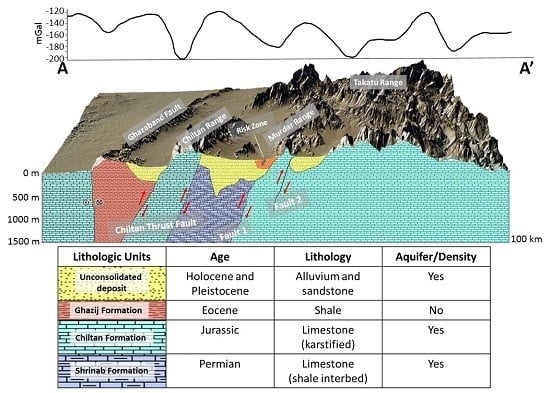
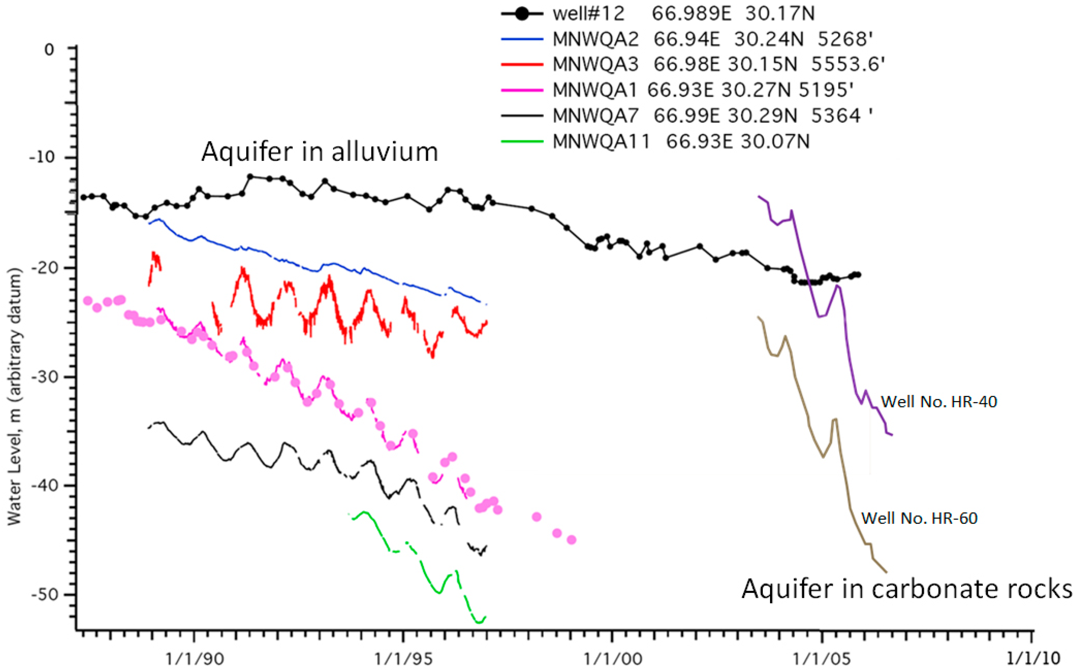
1.1. Aquifers of the Study Area

The city of Quetta has two primary aquifers that are bounded by alluvial sediments and carbonates. The bowl-shaped Quetta Valley is a landlocked watershed. The valley is mostly dry, and groundwater is the major source for domestic and agricultural utilization. The valley is syncline in nature and filled with thick alluvial deposits that include silt, clay, sand, and gravel. The dominant alluvial aquifers, which have an average thickness of ~300 m and a porosity of ~10%, are adjacent to the major mountain ranges: the Chiltan and Murdar Ranges [2]. The consolidated deposits of limestone, sandstone, and conglomerates are highly fractured, making aquifers, which are largely found in the Chiltan Formation and Shrinab Formation [20,21]. The Shrinab Formation is a deep aquifer composed of thick-bedded limestone with occasional shale and marl layers. The primary porosity of this zone is low, but due to tectonic activity and fracturing, secondary porosity has developed in this area. The majority of wells are used to extract water from the alluvium in the central part of the valley, while less water is extracted from the carbonate. These two aquifers are physically and hydraulically interconnected [1].

Up until 2010, there were 1619 wells for water withdrawal in Quetta [21]. The drilling depth of these wells was in the range of 100–200 m. Regular monitoring of the water table at various locations started in 1985 and has continued to the present in one form or another. Drilling has included many observation wells in regions where new production has been ongoing since 2000. From 1987–2006, the alluvial aquifer experienced a water level drop of ~1 m/year for a total decrease of ~18 m. Meanwhile, the carbonate aquifer experienced a total water level decline of ~20 m from 2003–2006, an average decline rate of ~5 m/year (Figure 2) [21].

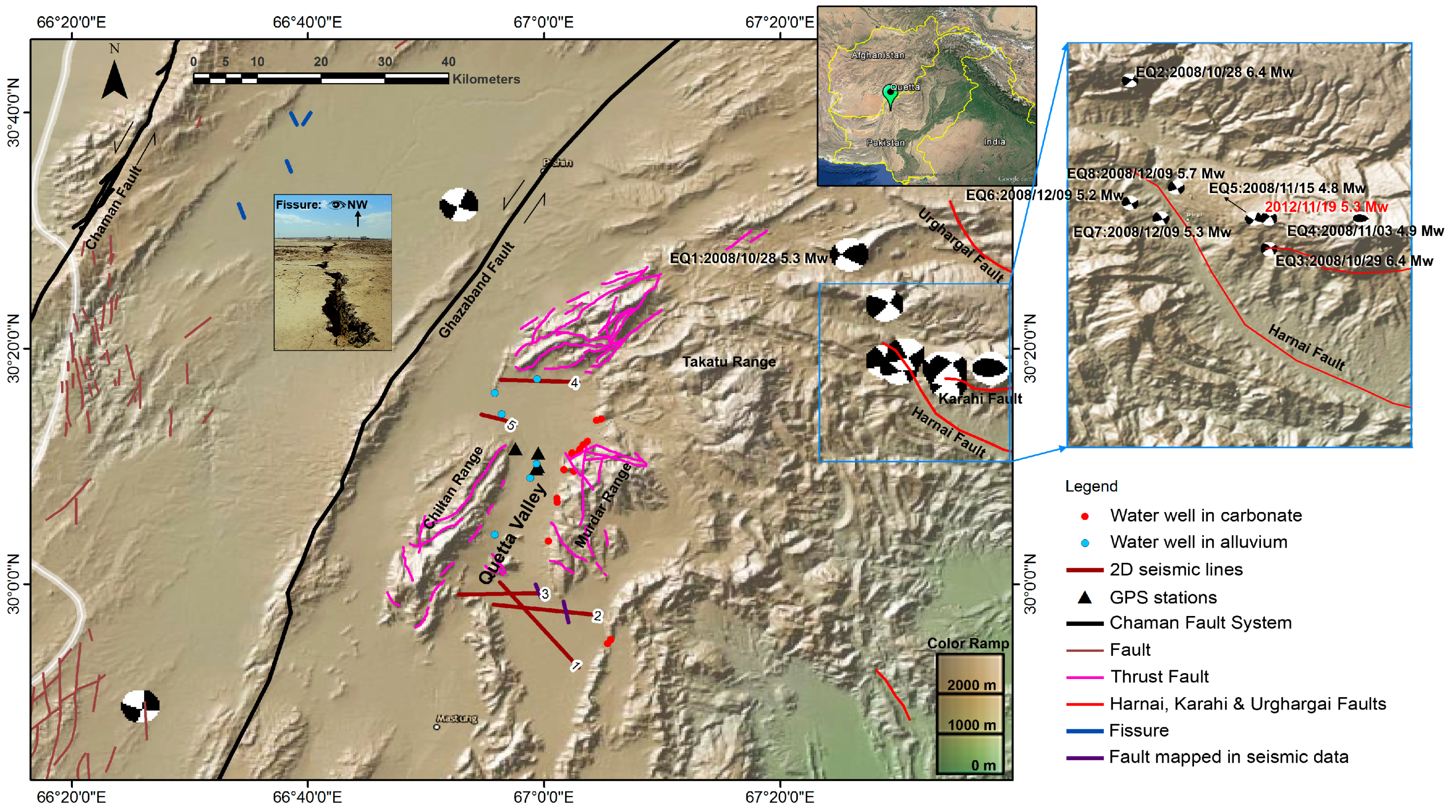
1.2. Quetta-Ziarat Earthquake Sequence

On 28–29 October 2008, three damaging and widely felt earthquakes (EQ) (EQ 1 Mw 5.3, EQ 2 Mw 6.4 and EQ 3 Mw 6.4) struck the rural, mountainous region of Quetta (Figure 1). Smaller magnitude EQ 4, 5, 6, 7 and 8 earthquakes subsequently occurred around the same location in November and December 2008. A total of eight earthquakes in this sequence had similar focal depths (~15 km). The fault plane solution determined by Global Centroid Moment Tensor (GCMT) solutions shows that the foreshock and main shock on 28–29 October occurred on a northwest–southeast-oriented right-lateral strike-slip motion with a steep dip (73°). Previous studies suggested that the earthquakes were caused by an unmapped right-lateral strike-slip fault and inferred basement faulting of 60 cm of total movement [22]. This unmapped fault could be the Urghargai Fault mapped by Kazmi [23] as an active right-lateral strike-slip fault striking in a northwest–southeast orientation (Figure 1).

2. Datasets and Methods

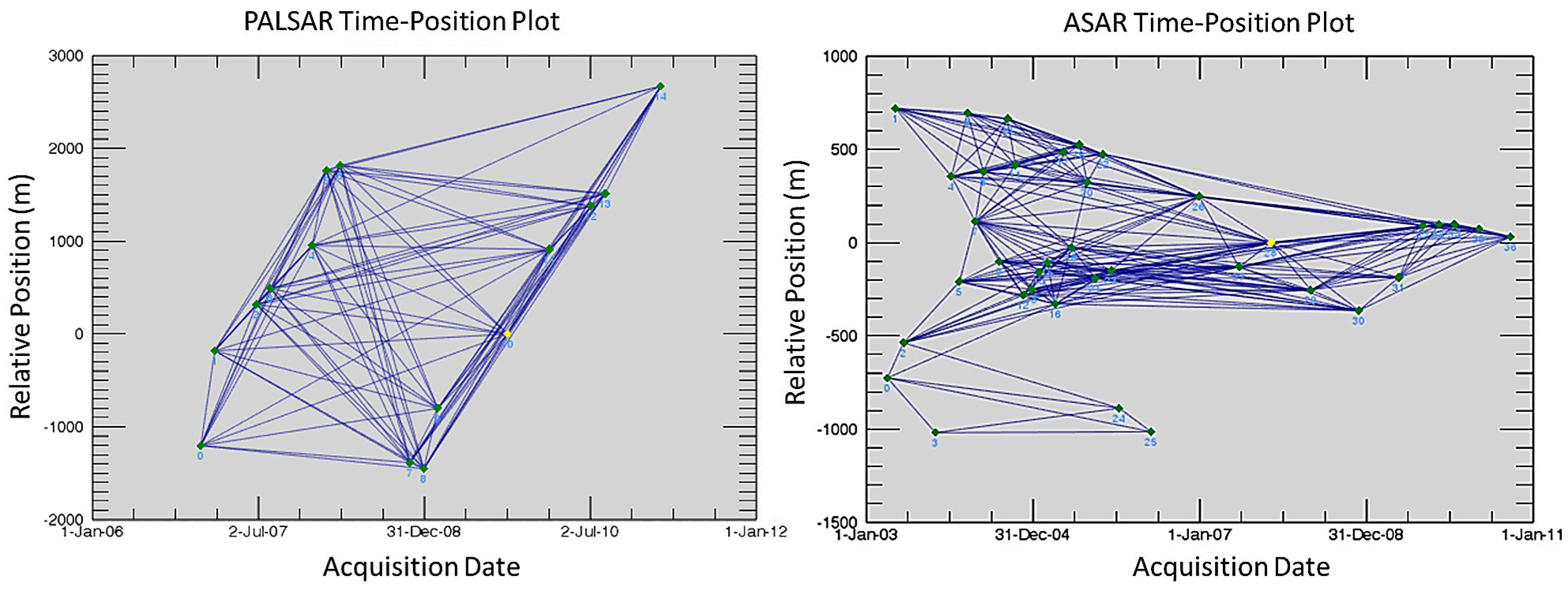
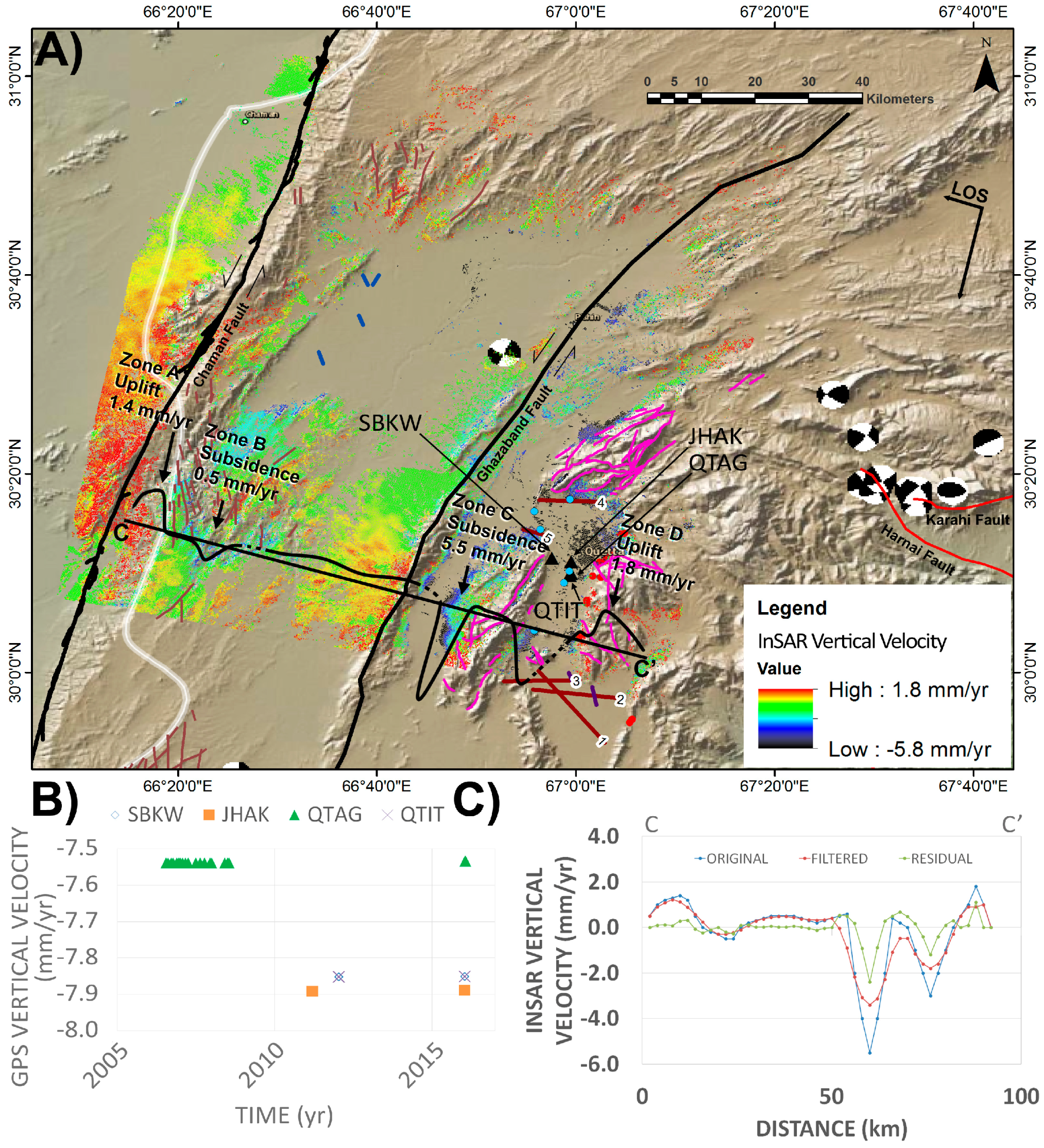
2.1. Interferometric Synthetic Aperture Radar (InSAR)

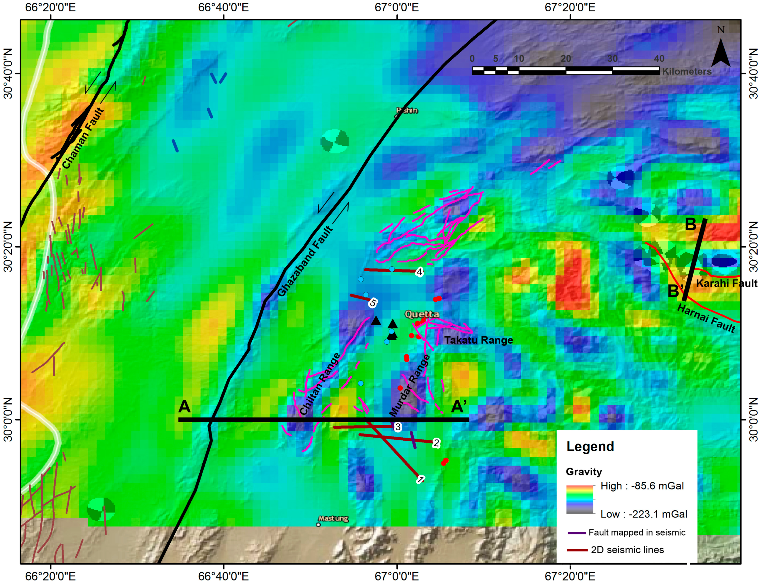
InSAR provides high-resolution geodetic measurements of surface deformations. A typical resolution for a phase measurement is about one-fifteenth of a phase cycle [24]. The interferometric stacking technique, Small Baseline Subset (SBAS), was used in this study to calculate surface deformation. The SBAS technique is based on a combination of differential interferograms produced by data pairs to derive surface deformation velocities by inversion of temporal phase profiles, effectively reducing atmospheric effects, topographic uncertainties, and orbital errors [25,26]. Images were processed using ENVI’s SARscape modules from EXELIS VIS Information Solutions.

Fifteen ascending Phased Array L-band Synthetic Aperture Radar (PALSAR) images acquired by an Advanced Land Observing Satellite (ALOS) with a ~23.6 cm wavelength were obtained from the Alaska Satellite Facility (ASF) and the Remote Sensing Technology Center of Japan (RESTEC); these images cover the time before and after the 2008 Quetta-Ziarat earthquake sequence (

Table 1. A list of Environmental Satellite (ENVISAT) Advanced Synthetic Aperture Radar (ASAR) and Advanced Land Observing Satellite (ALOS) Phased Array L-band Synthetic Aperture Radar (PALSAR) images used in Small Baseline Subset (SBAS) approach.

ENVISAT ASAR Descending 40 Images			ALOS PALSAR Ascending 15 Images
3 April 2003	18 November 2004	1 June 2006	24 December 2006
8 May 2003	23 December 2004	28 December 2006	8 February 2007
12 June 2003	27 January 2005	21 June 2007	26 June 2007
30 October 2003 (2 images)	3 March 2005	8 November 2007	11 August 2007
8 January 2004	7 April 2005	1 May 2008	27 December 2007
12 February 2004	12 May 2005 (2 images)	27 November 2008	11 February 2008
18 March 2004	16 June 2005	11 January 2009	28 March 2008
22 April 2004	21 July 2005	21 May 2009	13 November 2008
27 May 2004	25 August 2005	3 September 2009	29 December 2008
5 August 2004	29 September 2005	12 November 2009	13 February 2009
9 September 2004	3 November 2005	21 January 2010	1 October 2009
14 October 2004	8 December 2005	6 May 2010	16 February 2010
	12 January 2006	23 September 2010	4 July 2010
			19 August 2010
			19 February 2011

). A total of 97 interferogram pairs were generated using normal baseline thresholds of 50% of the critical baseline and 1200 days for the temporal baseline (Figure 3). Out of the 97 interferogram pairs, 53 pairs were chosen for further processing. Besides average velocity results, the incremental displacements by inversion of the temporal profile were also analyzed.

Forty descending ENVISAT Advanced Synthetic Aperture Radar (ASAR) images with a C-Band (~5.6 cm wavelength) covering the Quetta Valley from 2003–2010 were obtained from the European Space Agency (ESA) (Figure 1 and Figure 3). A total of 145 interferogram pairs were generated using normal baseline thresholds of 45% of the critical baseline for the spatial baseline and 1500 days for the temporal baseline. Out of 145 interferogram pairs, 93 pairs were chosen for further processing. The SBAS technique was also used to detect slow deformation in the Quetta Valley. Lastly, we estimated the mean crustal deformation velocity projected in a vertical direction as the final result.

The SBAS procedure includes co-registration, interferogram generation, flattening, and Goldstein filtering [27] with optimized parameters [28]. A complex multi-look operation was performed to produce a ground sampling distance of 80 m. A predefined linear displacement model was used to jointly estimate the DEM error and the low-pass displacement parameters [9,25,29,30] during the first inversion step. The atmospheric corrections were applied during second inversion step. An atmospheric filter was applied to smooth the signature of temporal displacement by using a low-pass spatial filter with a 1.2 km by 1.2 km window, which was followed by a high-pass temporal filter of 365 days [9,29]. GPS data were used to convert InSAR relative deformation to GPS-derived absolute deformation. GPS data with an actual measured deformation rate can be used as control points or reference points to convert InSAR relative deformation to GPS-like absolute deformation based on the offset and bias determined at GPS locations.

2.2. Gravity

Bouguer anomaly map was used to constrain the boundary of basins in the subsurface and identify regional structures. The gravity map shown in Figure 4 was compiled using a gravity database that included data from Sandwell et al. [31] for offshore regions and an Earth Gravitational Model (EGM2008) for terrestrial regions. The RMS error of the associated accuracy of EGM2008 is approximately ±1 mGal. The spatial resolution of the data is ~1.6 km. GEOSOFT Oasis Montaj software was used to obtain the gravity anomalies data. Gravity anomalies were used to map the crustal structure based on density contrasts. The gravity profiles along AA’ and BB’ were used for further analysis in Section 3.2 and Section 3.3.

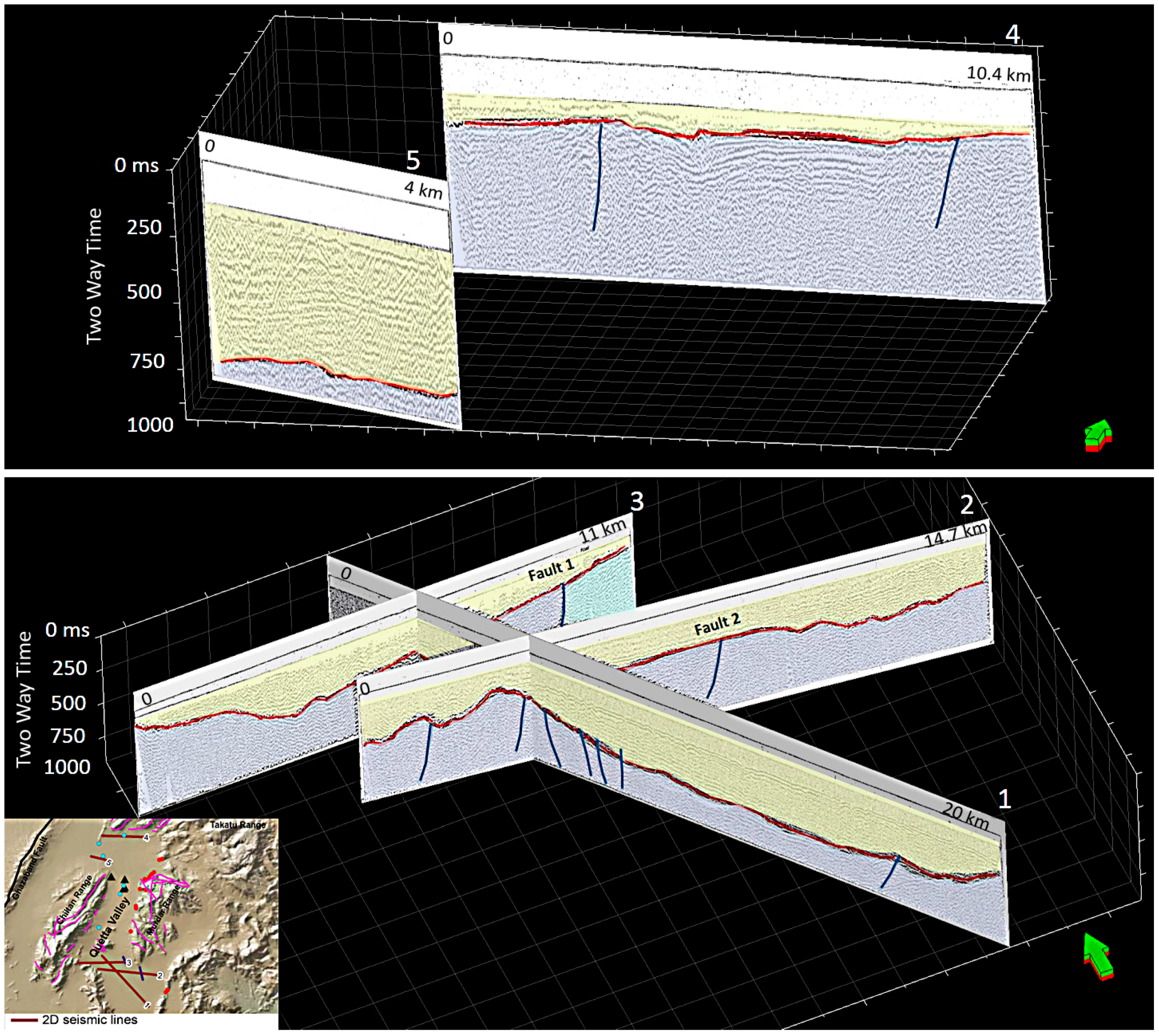
2.3. Two-Dimensional Seismic Profile

Five seismic reflection profiles were obtained from Techno Consult [32]. A single Vibroseis truck was used for data acquisition with a swept-frequency source ranging from 20–115 Hz and a 10–11 m distance between shots and geophones. All five seismic lines overlapped the ASAR images and were used to interpret the SBAS-InSAR surface displacement results (Figure 1). Data were acquired in 2003 with a total length of ~60 km. Profile 1 trends northwest–southeast, while profiles 2 and 3 both trend east–west, intersecting profile 1. North of Quetta, profile 4 and profile 5 both trend east–west. The seismic profiles were processed up to time-migrated images and interpreted for structural and stratigraphic information (Figure 5). Petrel Schlumberger software was used for interpretation with the assistance of published velocity models [33].

2.4. GPS

GPS data were collected in the Quetta Valley by the University of Balochistan from 2006–2016. Data were acquired using four GPS monitoring sites spread out in the valley: the Balochistan University IT Department (QTIT), the Balochistan University Geology Department (QTAG), Sardar Bahadur Khan University (SBKW), and Ismail House (IHAK) (Figure 1). As the stations were not continuously operating, GPS data were recorded at an interval of once per month or greater.

Raw data were first converted into a Rinex file format. The GPS data were then processed using the Automatic Precise Positioning Service (APPS) to get the GPS solution referenced in the International Terrestrial Reference Frame 2008 (ITRF 2008). Then, this output was rotated into an Indian-Plate-fixed reference frame with a pole-of-rotation calculation using a python code.

2.5. One-Dimensional Differential Compaction Theory

According to well-accepted theories [34], subsidence can be approximated by the following linear, simplified one-dimensional consolidation:

$$\delta =\alpha \times \omega \times s \times \mathsf{\Delta }h,$$

(1)

where δ (m) is subsidence, α (kg⁻¹·m⁻¹) is the compressibility of the soil, ω (kg) is the weight of water, s (m) is the sediment layer thickness, and ∆h (m) is the piezometric surface change.

First approximation, piezometric surface change is a linear function of sediment thickness:

$$\mathsf{\Delta }h=c_1 \times s$$

(2)

where c₁ is a constant.

Second approximation, the sediment layer thickness is a linear function of the distance from the basin margin:

$$s=c_2 \times x$$

(3)

where c₂ is a constant, and x is the distance from the basin margin.

Since the compressibility of the soil is constant, the weight of water is constant, and combines Equations (1)–(3):

$$\delta =c_3 \times x^2$$

(4)

where c₃ is a constant.

Based on the above two approximations, it indicates when the gradient of sediment thickness is constant, yielding the ratio:

$$\frac{d\delta }{dx}=c_4 \times x$$

(5)

where c₄ is a constant.

Above is the first scenario, in which the gradient of sediment thickness is constant. The second scenario occurs when the gradient of sediment thickness is considered a second order polynomial:

$$s=c_5 \times x^2$$

(6)

where c₅ is a constant.

By combining Equations (1), (2) and (6), we get,

$$\delta =c_6 \times x^4$$

(7)

where c₆ is a constant.

Similarly, we get the ratio:

$$\frac{d\delta }{dx}=c_7 \times x^3$$

(8)

where c₇ is a constant.

3. Results

3.1. SBAS Surface Displacement in the Quetta Valley

Figure 6 shows the vertical displacement velocity ranging from −5.8 mm/year to 1.8 mm/year averaged for seven years (3 April 2003–23 September 2010). There are fewer data points in the center of the footprint due to the low coherence of the images. On a descending path, the ENVISAT satellite moves south with its antenna pointed to the right. Therefore, a positive value can be regarded as an eastward shift, uplift, or both. We attributed this movement primarily to uplift for the following reasons: (1) From the general tectonics of the area, the region is subject to thrust and north–south strike-slip faults, intervening valleys, and basins. We could not resolve the north–south strike-slip Chaman Fault movement because of the Line of Sight (LOS) direction is perpendicular to the strike-slip movement direction. (2) The GPS observations from the stations deployed in the Quetta Valley during 2006–2016 indicate that the observed deformation is predominantly vertical movement (subsidence) [3,22].

The subsidence signal in the Quetta Valley was also recorded by GPS station recordings from 2006–2016, with an average subsidence rate of 7.7 mm/year. The InSAR results match the GPS rates, but with a smaller magnitude. This small discrepancy is likely due to the limitations of the spatial and temporal coverage caused by the intermittent GPS operation. GPS operates over a shorter time frame that does not involve continuous monitoring, whereas the InSAR result value involves a longer time frame and continuous monitoring and is therefore smaller. It is worth noting that InSAR-derived deformation velocity is a spatial average within a pixel (e.g., 80 m × 80 m), while GPS measurements represent a discrete point location. A 2D velocity profile CC’, which crosses zones A through D, was extracted from the SBAS-InSAR results. Profile CC’ shows zone A with 1.4 mm/year uplift, zone B with 0.5 mm/year subsidence (that could be noise), zone C with 5.5 mm/year subsidence, and zone D with 1.8 mm/year uplift (Figure 6A).

3.2. Structural Styles from Seismic Interpretation

Five time-migrated seismic reflection profiles were interpreted (Figure 5). The most distinguishable layer in the seismic profiles is the boundary between alluvium and limestone bedrock. A strong reflector, due to the high acoustic impedance contrast, characterizes this interface. The seismic profiles indicate that the high-angle thrust faults are mostly dipping westward. The descriptions of the interpreted seismic lines are as follows.

Seismic reflection profile 1 shows the depth to the bedrock (red-colored horizon), which is estimated to begin at a depth of ~380 m (Figure 5). A previous study showed that the bedrock is attributable to the Shrinab Formation, which has numerous reflectors that could be explained by alternating limestone and shale [20]. At the point where it intersects with profile 2, seismic profile 1 reveals a rising of the bedrock, which suggests complex folding in the bedrock affecting overlaying Quaternary alluvial deposits. In the middle portion of profile 2, the depth to the bedrock is ~240 m and increases to ~560 m at the eastern end. Profile 3 clearly shows the presence of a large asymmetric Quaternary basin up to ~500 m deep. Following the results of previous studies [20] and adding our new interpretations from the seismic data, a geological model along seismic profile 3 has been generated (Figure 7). The eastern part of profile 3 reveals what appears to be a thrust fault serving as the boundary between the Shrinab and the Chiltan Formations. Fault 1 was mapped on seismic profile 3 and fault 2 was mapped on seismic profile 2; both were projected onto the geologic model. The soft, unconsolidated nature of alluvial sediments in the Quetta Valley masked the bedrock fault scarps, but seismic reflection profiles helped to map these blind thrust faults.

Profile 4 intersects two blind thrust faults that dip west (Figure 5, Top). The Quaternary alluvial cover is thin along most of the line, rarely exceeding ~140 m. Profile 5 was difficult to interpret; although there are many reflectors, most are too weak to be clearly attributed to the bedrock, except for one at a depth of ~700 m that has been attributed to the top of the Shrinab Formation.

3.3. SBAS Co-Seismic Displacement at the 2008 Earthquake Epicenter

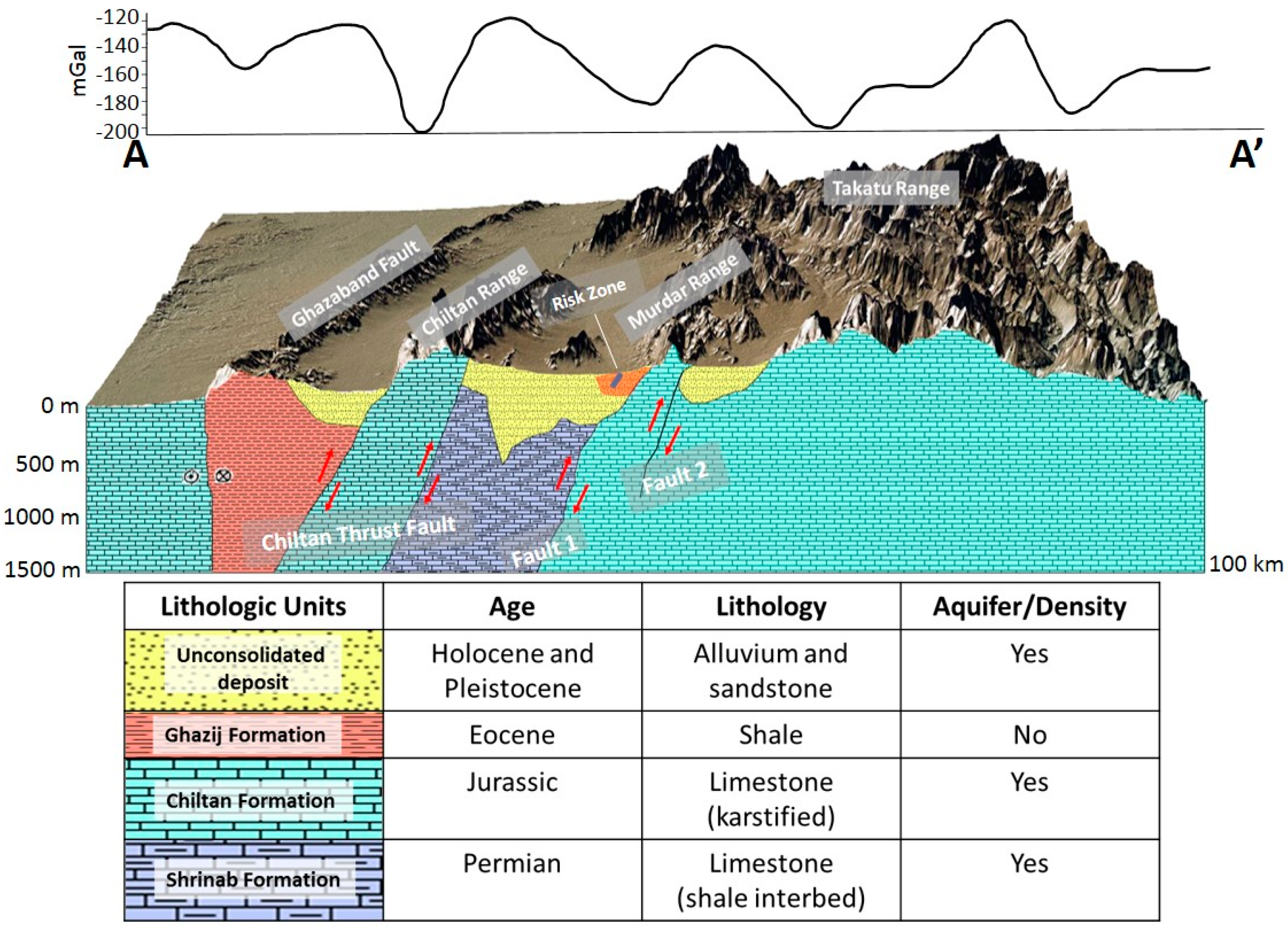
Figure 8A shows the Line of Sight (LOS) velocity ranging from −10 mm/year to 40 mm/year averaged for four years (24 December 2006–19 February 2011). On an ascending path, the ALOS-1 satellite moves north with its antenna pointed to the right. Therefore, a positive value can be regarded as a westward shift, uplift, or both. We attributed this movement primarily towards westward due to the strike-slip movement of Harnai and Karahi Faults.

The DInSAR for co-seismic event was also calculated (11 November 2008–29 December 2008), which shows the effect of EQ 5, 6, 7 and 8 (Figure 1) with a half fringe (a bright yellow dot in Supplementary file Figure S1) on the west side of the Harnai Fault suggesting ~55 mm of co-seismic displacement. Another fringe on the north side of the Harnai Fault can also be observed, but the time and location do not correspond to any of the eight earthquakes. This fringe could be caused by slow uplift of the Takatu Mountain Range.

3.4. Gravity

The Bouguer anomaly for the study area is between −85.6 and −223.1 mGal (Figure 4). The left side of the Chaman Fault shows relative high gravity (~−110 mGal), which may indicate that the depth to basement is shallow and/or thinner than crustal thickness. There are many metamorphic and volcanic rocks exposed along the Chaman Fault that may further support shallow basement depth [35]. Two trends and anomalies are clearly observable on the Bouguer map: (1) Between the Chaman Fault and the Ghazaband Fault, there are many linear patterns striking northeast–southwest with a small gravity gradient of ~1.5 mGal/km; (2) east of the Quetta Valley, there are nearly circular patterns with a high gravity gradient of ~8 mGal/km. The linear patterns may indicate folded structures in the Katawaz basin, and a small gravity gradient may indicate low-angle fold structures. The circular patterns with a relatively higher gradient of the Bouguer anomaly can be interpreted as a combination of high-angle basement faults and high-angle fold structures.

Two-dimensional Bouguer anomaly curves, AA’ and BB’, crossing the Quetta Valley, and the 2008 earthquake’s location were selected and analyzed for integration with the InSAR results (Figure 4). The Bouguer anomaly profile of AA’ shows highs and lows forming a trend likely related to mountain ranges and basins (Figure 7). Gravity profile BB’ across the Karahi and Harnai Faults shows a density change in the three blocks, which may indicate that they are each a different rock type (Figure 8B).

4. Discussion

4.1. Anthropogenic- versus Tectonic-Induced Subsidence

The Quetta Valley is a highly populated area (over 1.1 million residents as of 2016) and experiencing rapid population growth. Several earlier studies suggested that the excessive use of groundwater has caused subsidence in the valley [2,3]. The Quetta Valley is also located in an active tectonic region, along the boundary of the western Indian Plate. In order to assess the role of anthropogenic and tectonic processes in subsidence in the Quetta Valley, we adopted a novel technique that utilized a median filter commonly used in seismic data processing. A median filter operates by selecting the middle value of numbers within a window, which is then used as a geophysical tool for regional-residual separation [36,37].

Generally, tectonic deformation shows relatively slow movement rates over large regions [12,13] and can be considered as a long-wavelength background signal. In contrast, anthropogenic deformation has relative faster movement rates concentrated in smaller regions [3]; as such, this type of deformation can be considered as a short-wavelength localized signal. The terminology of long/short wavelengths is adopted here for the SBAS-InSAR distance–velocity profiles, not for the SBAS-InSAR time series profile. In other words, to separate the effects of tectonic processes from those of anthropogenic processes, only a distance profile on a regional scale can be used—a localized time series is not suitable.

A five-point median filter was applied to separate the short- and long-wavelength signals in order to assess the role of anthropogenic and tectonic processes on subsidence (Figure 6C). The filtered signal is the long wavelength, suggesting regional tectonics; whereas the residual signal is the short wavelength for the Quetta Valley, which is mainly caused by water withdrawal. The residual signal was calculated by subtracting the filtered signal from the original signal. In Figure 6C, the InSAR velocity profile shows uplift (1.4 mm/year) at zone A and may be subsidence at zone B, separated on the filtered curve (red-colored line). The displacements at zones A and B are relatively small—they could be noise. Because these zones are located along the transpression zone of the Chaman Fault and there are no urban areas, we considered that zones A and B are only affected by tectonic processes. On the other hand, zone C and zone D show subsidence and uplift on both the residual curve (green-colored line) and filtered curve (red-colored line) in the Quetta Valley (Figure 6C). This means that both tectonic and anthropogenic processes cause subsidence in zone C and uplift in zone D. Zone D covers the hanging wall of blind thrust fault 1 and 2 mapped by seismic profiles (Figure 6A); the creep along the thrust faults may cause accelerated uplift at zone D. There are studies showing that faults can also be reactivated and accelerated by water withdrawal in California, Arizona, and Houston [38,39,40].

The median filtered SBAS-InSAR distance–velocity profile revealed that the uplift and subsidence is mainly caused by tectonic processes in rural areas (zones A and B). In urban areas, both tectonic and anthropogenic processes contribute to the subsidence in the Quetta Valley (zones C and D). Anthropogenic processes include extensive water withdrawal and accelerated thrust fault movement due to water withdrawal. In zones A and B, we assume that the only contributions are from tectonic thrust faults, and that these regional contributions are homogeneous across the approximately 100 km span of profile CC’. A recent InSAR study along the Chaman Fault [41] found a relative thrust fault of movement around 2 mm/year further south toward the Nushki area.

Hence, the tectonic contributions of zones A and B are the same as those in the Quetta Valley in zones C and D. After removing the regional tectonic movement, we can see that the dominant subsidence in the Quetta Valley (zone C) is caused by water withdrawal. This same study [41] along the Chaman Fault also used InSAR velocity-distance profiles and found dominant subsidence caused by water withdrawal further north in the city of Qalat. Both the Qalat study and this study of Quetta Valley show the dominance of anthropogenic subsidence, which is masking the tectonic deformation.

4.2. Earthquake Displacement Interpretation

The Quetta-Ziarat 2008 earthquake swarms caused 215 deaths and left 200 injured. Previous studies have come up with different models for these earthquake swarms. Based on GPS data, previous work suggested a co-seismic slip of the northwest–southeast basement faulting in the earthquake sequence, but no surface rupture was found [22]. Using focal mechanisms analysis, other studies theorized that the northwest–southeast-oriented Urghargai Fault triggered the earthquakes [42,43]. Pinel-Puysségur et al. [44] and Pezzo et al. [45] provided a better explanation based on a two-image DInSAR technique and a forward modeling result. They proposed that the 2008 earthquake sequence was generated by two conjugate faults: a main northwest–southeast right-lateral strike-slip fault and a secondary northeast–southwest left-lateral strike-slip fault forming a “book shelf” structure.

However, using the SBAS-InSAR time series, gravity result, and the location of the two earlier mapped Harnai and Karahi Faults [46], we suggest a different explanation for the 2008 earthquake sequence. Compared with the two image DInSAR technique, the more comprehensive SBAS-InSAR time series results in this study show a right-lateral strike-slip movement of ~50 mm/year (including the co-seismic deformation) for the Harnai Fault and a left-lateral strike-slip movement of ~10 mm/year for the Karahi Fault (including the co-seismic deformation). Previous studies failed to take into consideration the known geological structures when developing their models, interpreted the focal mechanism fault plane into two northwest–southeast right-lateral and northeast–southwest left-lateral striking conjugate faults, and proposed the “book shelf” structure. Based on SBAS-InSAR result from this study and the northwest–southeast orientation of the Harnai and Karahi Faults, the northwest–southeast right-lateral focal mechanism fault plane is a more plausible explanation, since it is parallel to the Harnai and Karahi Faults.

Using these results and the gravity map, three zones were chosen at the earthquake locations along the Karahi and Harnai Faults for time series analysis. Figure 8C shows the time series for zone 1, with a significant increase in pre-seismic slip rates. Zone 2 and zone 3 had sinusoidal displacement patterns during the earthquake cycle. The positive velocity peak correspond to the 2008 earthquake swarms, where all three zones had sharp velocity drops and indicate a sharp release of strain. Zone 2 had a faster westward movement compared to zone 1, which indicates the Karahi Fault may have switched into a right-lateral movement during the earthquake swarms. This explains the right-lateral focal mechanism (EQ 3, 4 and 5, Figure 1) around the Karahi Fault. The Harnai and Karahi Faults correspond to the earthquake locations and may be easily extended further north to match the observed two right-lateral earthquakes from the earthquake sequence in that area (EQ 1 and 2, Figure 1). Zones 2 and 3 have sinusoidal displacement patterns that demonstrate the accumulation and release of strain on the Harnai and Karahi Faults during the earthquake cycle. The Harnai and Karahi Faults both had right-lateral movement during the 2008 earthquake swarms. Leeman et al. [47] found similar results in their laboratory experiments while simulating slow-slip behaviors for faults. Although due to different tectonic scenarios and rock friction properties, the inter-seismic strain patterns are different and vary by location [48]. Even at the same location, the amplitude and period of the pattern varies, which is a major obstacle to implementing the pre-seismic displacement pattern in seismic hazard prediction. However, the sinusoidal displacement patterns at the Quetta-Ziarat earthquake location may suggest an association between tectonic displacement and earthquakes in the Quetta Valley.

4.3. Ground Fissures Interpretation and Zone of Potential Failure

The ground fissures that appeared in February 2011 near the Quetta Valley are forming a conjugate set, and the maximum principal stress axis is pointing north. These Coulomb-type conjugate fissures show that the orientation is controlled by the regional maximum principal stress field according to the Coulomb failure criterion in this region [49].

Ground subsidence due to sediment compaction following fluid withdrawal is a widely known effect. The remaining problem is the correlation of active faults with ground fissures, a correlation which has led some investigators to interpret the latter, at least partly, as tectonic effects; and, in particular, as evidence of aseismic creep. Kontogianni et al. [50] showed that, in Greece, fissures can be controlled by bedrock faulting and differential compaction in areas of ongoing water-level decline and subsidence. Equations (5) and (8) (Section 2.5) demonstrates that the gradient of subsidence increases exponentially due to the gradient of sediment thickness. This was used to identify potential risk zone for fissures in Figure 7.

The risk zone is defined based on the blind fault 1 mapped from the seismic profile (see Figure 5). The InSAR results show fault creep and local uplift (1.8 mm/year) near fault 1 and other pre-existing thrust faults in the Murdar Mountain Range (Figure 6A). Unlike other blind faults mapped from the seismic profiles, fault 1 is active beneath the alluvium, and the location of fault 1 may be a main control of alluvial thickness at that location (Figure 7). This is why we consider the risk zone to be close to the Murdar Mountain Range and not near the Chiltan Mountain Range or in other basins. In Figure 7, the location for fissures is parallel to faults in the carbonates and, as such, is considered a high-risk location.

In other words, three factors control the occurrence of fissures in the Quetta Valley: (1) the regional stress field; (2) sediment compaction; and (3) active bedrock faulting. Ground fissures that appeared in February 2011 were most likely caused by the regional stress field and sediment compaction, and were thus not related to the earthquakes.

5. Conclusions

Data from InSAR, seismic profiles, and gravity were used to map the surface deformation caused by subsidence and earthquake swarms in the Quetta Valley and surrounding vicinities.

• InSAR results from 2003–2010 show a rate of 5.5 mm/year for subsidence in the Quetta Valley and a rate of 1.8 mm/year for uplift in the mountain ranges surrounding the valley. A median filter was applied to the InSAR velocity curve to separate the subsidence caused by tectonic processes from subsidence caused by anthropogenic processes. The results indicate subsidence in the Quetta Valley is mainly caused by anthropogenic processes followed by movement along thrust faults.
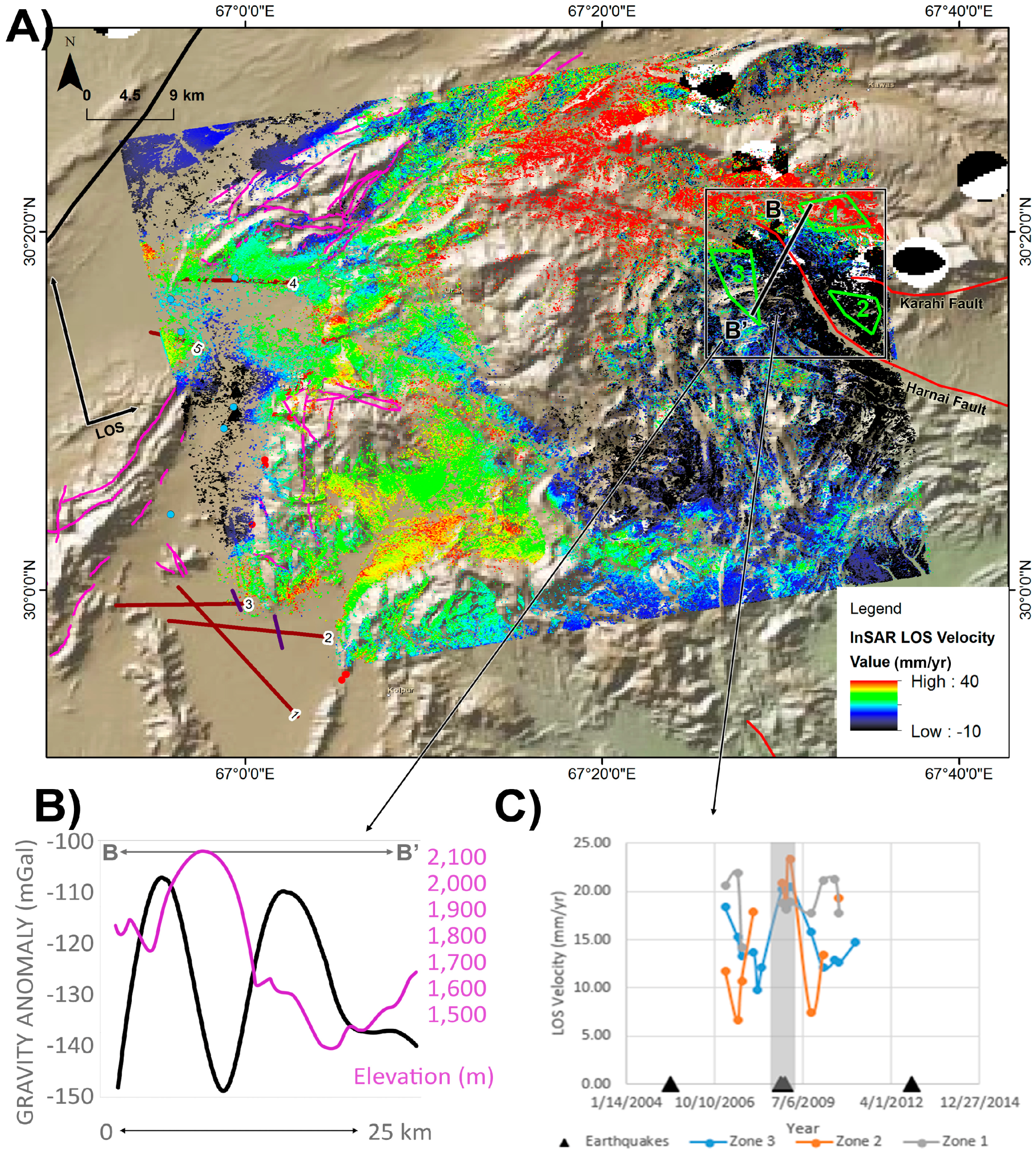
• Multi-temporal InSAR analysis shows a sinusoidal displacement pattern for the swarm of earthquakes that occurred in 2008 along the Harnai and Karahi strike-slip faults.
• This study identified a high risk for potential fissures.

References

1. Kazmi, A.H.; Jan, M.Q. Geology and Tectonics of Pakistan; Graphic publishers: Brisbane, Australia, 1997. [Google Scholar]
2. Water and Power Development Authority. Individual Basinal Reports of Balochistan, Hydrogelogy Project, Quetta, 1982–2000, Pakistan; Water and Power Development Authority: Lahore, Pakistan, 2001.
3. Khan, A.S.; Khan, S.D.; Kakar, D.M. Land subsidence and declining water resources in Quetta Valley, Pakistan. Environ. Earth Sci. 2013, 70, 2719–2727. [Google Scholar] [CrossRef]
4. Mohadjer, S.; Bendick, R.; Ischuk, A.; Kuzikov, S.; Kostuk, A.; Saydullaev, U.; Lodi, S.; Kakar, D.; Wasy, A.; Khan, M. Partitioning of India-Eurasia convergence in the Pamir-Hindu Kush from GPS measurements. Geophys. Res. Lett. 2010, 37. [Google Scholar] [CrossRef]
5. Furuya, M.; Satyabala, S. Slow earthquake in Afghanistan detected by InSAR. Geophys. Res. Lett. 2008, 35. [Google Scholar] [CrossRef]
6. Bannert, D.; Cheema, A.; Ahmed, A.; Schäffer, U. The structural development of the western fold thrust belt, Pakistan. Geol. Jahrbuch Reihe 1992, 80, 1–60. [Google Scholar]
7. Engelkemeir, R.; Khan, S.D.; Burke, K. Surface deformation in Houston, Texas using GPS. Tectonophysics 2010, 490, 47–54. [Google Scholar] [CrossRef]
8. Qu, F.; Lu, Z.; Zhang, Q.; Bawden, G.W.; Kim, J.-W.; Zhao, C.; Qu, W. Mapping ground deformation over Houston-Galveston, Texas using multi-temporal InSAR. Remote Sens. Environ. 2015, 169, 290–306. [Google Scholar] [CrossRef]
9. Grzovic, M.; Ghulam, A. Evaluation of land subsidence from underground coal mining using TimeSAR (SBAS and PSI) in Springfield, Illinois, USA. Nat. Hazards 2015, 79, 1739–1751. [Google Scholar] [CrossRef]
10. Yin, Y.; Zhang, K.; Li, X. Urbanization and land subsidence in China. China Geol. Surv. 2006, 31, 1–5. [Google Scholar]
11. Galloway, D.; Jones, D.R.; Ingebritsen, S.E. Land Subsidence in the United States; US Geological Survey: Reston, VA, USA, 1999.
12. Ivins, E.R.; Dokka, R.K.; Blom, R.G. Post-glacial sediment load and subsidence in coastal Louisiana. Geophys. Res. Lett. 2007, 34. [Google Scholar] [CrossRef]
13. Royden, L.; Keen, C. Rifting process and thermal evolution of the continental margin of eastern Canada determined from subsidence curves. Earth Planet. Sci. Lett. 1980, 51, 343–361. [Google Scholar] [CrossRef]
14. Khan, S.D.; Huang, Z.; Karacay, A. Study of ground subsidence in northwest Harris county using GPS, LiDAR, and InSAR techniques. Nat. Hazards 2014, 1–31. [Google Scholar] [CrossRef]
15. Coplin, L.S.; Galloway, D. Houston-Galveston, Texasas—Managing coastal subsidence. In Land Subsidence in the United States; Galloway, D.L., Jones, D.R., Ingebritsen, S.E., Eds.; US Geological Survey Circular: Reston, VA, USA, 1999; pp. 35–48. [Google Scholar]
16. O’Neill, M.; Van Siclen, D. Activation of Gulf Coast faults by depressuring of aquifers and an engineering approach to siting structures along their traces. Bull. Assoc. Eng. Geol. 1984, 21, 73–87. [Google Scholar]
17. Jones, A.; Manistre, B.; Oliver, R.; Willson, G.; Scott, H. Reconnaissance Geology of Part of West Pakistan (Colombo Plan Co-Operative Project Conducted and Compiled by Hunting Survey Corporation); Government of Canada: Toronto, ON, Canada, 1960.
18. GeoMapApp. Available online: http://www.geomapapp.org (accessed on 1 June 2016).
19. Ryan, W.B.; Carbotte, S.M.; Coplan, J.O.; O’Hara, S.; Melkonian, A.; Arko, R.; Weissel, R.A.; Ferrini, V.; Goodwillie, A.; Nitsche, F. Global multi-resolution topography synthesis. Geochem. Geophys. Geosyst. 2009. [Google Scholar] [CrossRef]
20. Sagintayev, Z.; Sultan, M.; Khan, S.D.; Khan, S.A.; Mahmood, K.; Yan, E.; Milewski, A.; Marsala, P. A remote sensing contribution to hydrologic modelling in arid and inaccessible watersheds, Pishin Lora basin, Pakistan. Hydrol. Process. 2012, 26, 85–99. [Google Scholar] [CrossRef]
21. Halcrow and Cameos Consultant Companies. Groundwater Management Plan for Quetta Sub-Basin; Balochistan Irrigation and Power Department: Quetta, Pakistan, 2010.
22. Khan, M.A.; Bendick, R.; Bhat, M.I.; Bilham, R.; Kakar, D.M.; Khan, S.F.; Lodi, S.H.; Qazi, M.S.; Singh, B.; Szeliga, W. Preliminary geodetic constraints on plate boundary deformation on the western edge of the Indian plate from TriGGnet (Tri-University GPS Geodesy Network). J. Himal. Geosci. 2008, 41, 71–87. [Google Scholar]
23. Kazmi, A.H. Active fault systems in Pakistan. Geodyn. Pak. 1979, 1979, 285–294. [Google Scholar]
24. Zebker, H.A.; Rosen, P.A.; Goldstein, R.M.; Gabriel, A.; Werner, C.L. On the derivation of coseismic displacement fields using differential radar interferometry: The Landers earthquake. J. Geophys. Res. Solid Earth (1978–2012) 1994, 99, 19617–19634. [Google Scholar] [CrossRef]
25. Berardino, P.; Fornaro, G.; Lanari, R.; Sansosti, E. A new algorithm for surface deformation monitoring based on small baseline differential SAR interferograms. IEEE Trans. Geosci. Remote Sens. 2002, 40, 2375–2383. [Google Scholar] [CrossRef]
26. Lanari, R.; Mora, O.; Manunta, M.; Mallorquí, J.J.; Berardino, P.; Sansosti, E. A small-baseline approach for investigating deformations on full-resolution differential SAR interferograms. IEEE Trans. Geosci. Remote Sens. 2004, 42, 1377–1386. [Google Scholar] [CrossRef]
27. Goldstein, R.M.; Werner, C.L. Radar interferogram filtering for geophysical applications. Geophys. Res. Lett. 1998, 25, 4035–4038. [Google Scholar] [CrossRef]
28. Ghulam, A.; Amer, R.; Ripperdan, R. A filtering approach to improve deformation accuracy using large baseline, low coherence DInSAR phase images. In Proceedings of the 2010 IEEE International Geoscience and Remote Sensing Symposium (IGARSS), Honolulu, HI, USA, 25–30 July 2010; pp. 3494–3497.
29. Abir, I.A.; Khan, S.D.; Ghulam, A.; Tariq, S.; Shah, M.T. Active tectonics of western Potwar Plateau—Salt Range, northern Pakistan from InSAR observations and seismic imaging. Remote Sens. Environ. 2015, 168, 265–275. [Google Scholar] [CrossRef]
30. Lauknes, T.; Shanker, A.P.; Dehls, J.; Zebker, H.; Henderson, I.; Larsen, Y. Detailed rockslide mapping in northern Norway with small baseline and persistent scatterer interferometric SAR time series methods. Remote Sens. Environ. 2010, 114, 2097–2109. [Google Scholar] [CrossRef]
31. Sandwell, D.T.; Müller, R.D.; Smith, W.H.; Garcia, E.; Francis, R. New global marine gravity model from CryoSat-2 and Jason-1 reveals buried tectonic structure. Science 2014, 346, 65–67. [Google Scholar] [CrossRef] [PubMed]
32. Quetta Water Supply and Environmental Improvement Project. Available online: https://www.adb.org/projects/documents/quetta-water-supply-and-environmental-improvement-project (accessed on 16 November 2016).
33. Alam, K.; Ahmad, N. Determination of aquifer geometry through geophysical methods: A case study from Quetta Valley, Pakistan. Acta Geophys. 2014, 62, 142–163. [Google Scholar] [CrossRef]
34. Gambolat, G.; Freeze, R. Mathmatical Simulation of Subsidence of Venice; Transactions-American Geophysical Union, 1973; American Geophysical Union: Washington, DC, USA, 1973; p. 214. [Google Scholar]
35. Lawrence, R.; Yeats, R.; Khan, S.; Subhani, A.; Bonelli, D. Crystalline rocks of the Spinatizha area, Pakistan. J. Struct. Geol. 1981, 3, 449–457. [Google Scholar] [CrossRef]
36. Stewart, R.R. Median filtering: Review and a new F/K analogue design. J. Can. Soci. Explor. Geophys. 1985, 21, 54–63. [Google Scholar]
37. Kim, S.S.; Wessel, P. Directional median filtering for regional-residual separation of bathymetry. Geochem. Geophys. Geosyst. 2008. [Google Scholar] [CrossRef]
38. Holzer, T.L. Faulting caused by groundwater level declines, San Joaquin Valley, California. Water Resour. Res. 1980, 16, 1065–1070. [Google Scholar] [CrossRef]
39. Huang, J.; Van Nieuwenhuise, D.; Khan, S.D. Integrated fault and hazard analysis in Downtown Houston, Texas. GCAGS J. 2015, 4, 147–154. [Google Scholar]
40. Holzer, T.L.; Davis, S.N.; Lofgren, B.E. Faulting caused by groundwater extraction in southcentral Arizona. J. Geophys. Res. Solid Earth (1978–2012) 1979, 84, 603–612. [Google Scholar] [CrossRef]
41. Fattahi, H.; Amelung, F. InSAR observations of strain accumulation and fault creep along the Chaman Fault system, Pakistan and Afghanistan. Geophys. Res. Lett. 2016. [Google Scholar] [CrossRef]
42. Yadav, R.; Gahalaut, V.; Chopra, S.; Shan, B. Tectonic implications and seismicity triggering during the 2008 Baluchistan, Pakistan earthquake sequence. J. Asian Earth Sci. 2012, 45, 167–178. [Google Scholar] [CrossRef]
43. Monalisa, Q.J. Geoseismological study of the Ziarat (Balochistan) Earthquake (Doublet?) of October 28, 2008. Curr. Sci. 2010, 98, 50–57. [Google Scholar]
44. Pinel-Puysségur, B.; Grandin, R.; Bollinger, L.; Baudry, C. Multifaulting in a tectonic syntaxis revealed by InSAR: The case of the Ziarat earthquake sequence (Pakistan). J. Geophys. Res. Solid Earth 2014, 119, 5838–5854. [Google Scholar] [CrossRef]
45. Pezzo, G.; Boncori, J.P.M.; Atzori, S.; Antonioli, A.; Salvi, S. Deformation of the western Indian Plate boundary: Insights from differential and multi-aperture InSAR data inversion for the 2008 Baluchistan (Western Pakistan) seismic sequence. Geophys. J. Int. 2014, 198, 25–39. [Google Scholar] [CrossRef]
46. Lawrence, R.D.; Yeats, R.S. Geological reconnaissance of the Chaman Fault in Pakistan. Geodyn. Pak. 1979, 9, 351–357. [Google Scholar]
47. Leeman, J.; Saffer, D.; Scuderi, M.; Marone, C. Laboratory observations of slow earthquakes and the spectrum of tectonic fault slip modes. Nat. Commun. 2016. [Google Scholar] [CrossRef] [PubMed]
48. Fialko, Y. Interseismic strain accumulation and the earthquake potential on the southern San Andreas fault system. Nature 2006, 441, 968–971. [Google Scholar] [CrossRef] [PubMed]
49. Turner, J.P.; Williams, G.A. Sedimentary basin inversion and intra-plate shortening. Earth-Sci. Rev. 2004, 65, 277–304. [Google Scholar] [CrossRef]
50. Kontogianni, V.; Pytharouli, S.; Stiros, S. Ground subsidence, Quaternary faults and vulnerability of utilities and transportation networks in Thessaly, Greece. Environ. Geol. 2007, 52, 1085–1095. [Google Scholar] [CrossRef]
Figure 1. Map of major structures and earthquake hypocenters for the Quetta Valley and surrounding areas. The focal mechanisms of the October–December 2008 earthquakes are shown. Thrust faults in the Quetta Valley from Jones et al. [17] are also shown. Two blind thrust faults identified using 2D seismic data are shown in indigo. The beach ball symbol indicates the centroid-moment-tensor (CMT) solution [18,19].
Remotesensing 08 00956 g001
Figure 2. Water level decline from 1987–2006 in alluvial and carbonate aquifers of Quetta Valley [21]. The hydrographs of these wells clearly indicate a constant decline in their water levels. The water level decline rate was lower at ~1 m/year in alluvial aquifers and higher at ~5 m/year in carbonate aquifers. Locations of water wells in alluvium and carbonate are indicated by blue and red dots, respectively, in Figure 1.
Remotesensing 08 00956 g002
Figure 3. Normal baselines (y-axis) and the acquisition dates (x-axis). The yellow diamonds refer to the Small Baseline Subset (SBAS) super master image (1 October 2009, for Phased Array L-band Synthetic Aperture Radar (PALSAR) and 8 November 2007, for Advanced Synthetic Aperture Radar (ASAR).
Remotesensing 08 00956 g003
Figure 4. Bouguer gravity anomaly ranging from −85.6 to −223.1 mGal shows the crustal density variations in the Quetta Valley and surrounding areas. AA’ is a 2D gravity profile used in Figure 7, and BB’ is a 2D gravity profile extracted across the Karahi and Harnai Faults, shown in Figure 8.
Remotesensing 08 00956 g004
Figure 5. (Top) Seismic profile 4 and 5 show the top of Shrinab Limestone (red horizons) and two thrust faults, shown on profile 4, dipping westward. (Bottom) Seismic profile 1, 2 and 3 show the top of Shrinab Limestone (red horizons) and many blind thrust faults. Only one thrust fault mapped on profile 3 serves as a boundary between the Shrinab and Chiltan Formations.
Remotesensing 08 00956 g005
Figure 6. (A) SBAS results generated from forty descending ENVISAT ASAR images from 2003–2010 show surface deformations ranging from −5.8–1.8 mm/year in the Quetta Valley and surrounding areas. A 2D velocity profile, CC’, was extracted from the InSAR results. The low coherence area is marked by a dotted line on the CC’ velocity profile. (B) GPS rates from 2006–2016 in a vertical direction around –7.7 mm/year, which matches the InSAR vertical movement rate in the Quetta Valley. (C) A five-point median filter was applied on the CC’ cross-profile (Figure 6A) to distinguish the subsidence caused by tectonic processes (shown as a red line) from subsidence caused by anthropogenic processes (water withdrawal) (shown as a green line).
Remotesensing 08 00956 g006
Figure 7. Schematic cross-section AA’ (parallel with seismic profile 3) modified from a previous study [20] to explain subsidence in the Quetta Valley and surrounding areas. The Bouguer anomaly profile of AA’ shows highs and lows forming a trend likely related to mountain ranges and basins. This model shows the activity of blind thrust faults 1 and 2 mapped in subsurface using 2D seismic profiles, which are part of the Chiltan Thrust System. High-risk locations for potential fissures are shown near the Murdar Range based on differential compaction theory in Section 2.5.
Remotesensing 08 00956 g007
Figure 8. (A) SBAS results generated from 15 ascending PALSAR scenes from 2006 to 2011 show a surface deformation velocity ranging from −10–40 mm/year. (B) The profile BB’ shows changes in gravity across the Karahi and Harnai Faults. The gravity data indicate the presence of three different fault blocks that cross faults. (C) The SBAS multi-temporal analysis shows a change in pre-, co-, and post-seismic velocity rates for zones 1, 2 and 3 at the epicenters of the 2008 earthquake swarms.
Remotesensing 08 00956 g008