Article

Mapping Annual Forest Cover in Sub-Humid and Semi-Arid Regions through Analysis of Landsat and PALSAR Imagery

1
Department of Microbiology and Plant Biology, Center for Spatial Analysis, University of Oklahoma, Norman, OK 73019, USA
2
Ministry of Education Key Laboratory of Biodiversity Science and Ecological Engineering, Institute of Biodiversity Science, Fudan University, Shanghai 200433, China
3
Oklahoma Natural Heritage Inventory, Department of Geography and Environmental Sustainability, University of Oklahoma, Norman, OK 73019, USA
4
Environmental Division, Arkansas State Highway and Transportation Department, Little Rock, AR 72209, USA
5
Oklahoma Biological Survey, University of Oklahoma, Norman, OK 73019, USA
6
Oklahoma Forestry Services, Oklahoma city, OK 73105, USA
7
U.S. Geological Survey (USGS) Earth Resources Observation and Science (EROS) Center, Sioux Falls, SD 57198, USA
*
Author to whom correspondence should be addressed.
Remote Sens. 2016, 8(11), 933; https://doi.org/10.3390/rs8110933
Submission received: 22 September 2016 / Revised: 25 October 2016 / Accepted: 3 November 2016 / Published: 10 November 2016

Abstract

:
Accurately mapping the spatial distribution of forests in sub-humid to semi-arid regions over time is important for forest management but a challenging task. Relatively large uncertainties still exist in the spatial distribution of forests and forest changes in the sub-humid and semi-arid regions. Numerous publications have used either optical or synthetic aperture radar (SAR) remote sensing imagery, but the resultant forest cover maps often have large errors. In this study, we propose a pixel- and rule-based algorithm to identify and map annual forests from 2007 to 2010 in Oklahoma, USA, a transitional region with various climates and landscapes, using the integration of the L-band Advanced Land Observation Satellite (ALOS) PALSAR Fine Beam Dual Polarization (FBD) mosaic dataset and Landsat images. The overall accuracy and Kappa coefficient of the PALSAR/Landsat forest map were about 88.2% and 0.75 in 2010, with the user and producer accuracy about 93.4% and 75.7%, based on the 3270 random ground plots collected in 2012 and 2013. Compared with the forest products from Japan Aerospace Exploration Agency (JAXA), National Land Cover Database (NLCD), Oklahoma Ecological Systems Map (OKESM) and Oklahoma Forest Resource Assessment (OKFRA), the PALSAR/Landsat forest map showed great improvement. The area of the PALSAR/Landsat forest was about 40,149 km2 in 2010, which was close to the area from OKFRA (40,468 km2), but much larger than those from JAXA (32,403 km2) and NLCD (37,628 km2). We analyzed annual forest cover dynamics, and the results show extensive forest cover loss (2761 km2, 6.9% of the total forest area in 2010) and gain (3630 km2, 9.0%) in southeast and central Oklahoma, and the total area of forests increased by 684 km2 from 2007 to 2010. This study clearly demonstrates the potential of data fusion between PALSAR and Landsat images for mapping annual forest cover dynamics in sub-humid to semi-arid regions, and the resultant forest maps would be helpful to forest management.

Graphical Abstract

1. Introduction

In sub-humid and semi-arid regions, forests play an important role in protecting the land from degradation and conserving biodiversity; however, they are vulnerable to degradation due to low rainfall and deforestation, including the overexploitation of trees from clear-cutting forests for agricultural and logging purposes [1]. Relatively large uncertainties still exist in the spatial distribution of forests and deforestation, especially in sub-humid and semi-arid regions with low forest canopy coverage [2,3], which may result in large discrepancy in the estimation of forest biomass and carbon emission [4,5]. Therefore, accurate forest distribution maps with low uncertainties are critical to assessing the forest change in these regions and understanding the role of forests in providing valuable ecosystem services, thus supporting the policy towards Reducing Emissions from Deforestation and Forest Degradation (REDD+).
Remote sensing has been widely applied for mapping the spatio-temporal patterns of forests from local to global scales. Such applications are quite valuable in regions that are remote with limited forest information. Past studies have generated forest maps primarily from optical remote sensing imagery, including 8- or 1-km Advanced Very High Resolution Radiometer (AVHRR) [6,7], 500-m Moderate Resolution Imaging Spectroradiometer (MODIS) [8,9,10], and 30-m Landsat TM/ETM+ images [11,12]. Although the 500-m, 1-km, and 8-km forest maps adequately describe the general patterns of the spatial distribution of forests and forest change, these coarse resolution datasets have limited utility in fragmented landscapes. Landsat imagery has been widely used for regional and global forest mapping and land cover classification [11,12,13,14,15]. These 30-m forest products provide more detail in the spatial distribution of forests and forest change than those derived from AVHRR and MODIS datasets.
Active microwave remote sensing has the advantage of the all-weather capability to map land surfaces and has been widely used for forest mapping. L-band synthetic aperture radar (SAR) data have relatively longer band wavelength, greater penetration into forests, and stronger volume scattering signals than that of X- and C-band sensors. It exhibits substantial volume scattering and great sensitivity to the biomass and structure of forests as incident energy interacts with large trunk and branch components [16,17,18], and is preferred for forest mapping. Japan Earth Resources Satellite 1 (JERS-1) images (1992–1998) were the first L-band SAR used for forest mapping at the continental scale. JERS-1 was evaluated with stable backscatter values in both wet and dry seasons in different years in the southwest Amazon [19] and were applied for mapping tropical forests [20,21,22]. The freely available Advanced Land Observation Satellite (ALOS) Phased Array type L-band Synthetic Aperture Radar (PALSAR) and ALOS-2 PALSAR-2 offer wall-to-wall forest mapping capability [23], and have been used to detect hotspots of forest cover changes (gain or loss of forest cover) [24,25,26]. C- and X-band SAR have also been used for forest mapping [27]. However, their signals are often saturated at the canopy, making it difficult to distinguish forests from crops.
Both optical and SAR remote sensing face certain challenges for accurately mapping forests. Optical remote sensing imagery has been consistently available since the early 1970s and is a major data source for historic forest mapping. However, the utility of optical remote sensing images is often limited by the quality of observations (e.g., cloud and cloud shadow) [28]. To overcome this problem, imagery from multiple years can increase the number of good-quality observations for forest mapping, although combining images from multiple years diminishes the temporal sensitivity for the detection of forest change [11]. Forests are also easily confused with some other land cover types (e.g., shrub), as they have similar phenology and greenness features [29,30]. The SAR-based forest maps tend to include some commission errors from buildings and rocky land due to similarities in the structure of features. Previous studies introduced the potential of the integration of SAR and optical remote sensing images for mapping ice shelf change, urban areas, crops, forest biomass, and forest disturbance [18,31,32,33,34]. Therefore, the integration of SAR and optical remote sensing images may improve the accuracy of forest mapping, as demonstrated in several recent studies [35,36,37].
This study took place in Oklahoma—a region dominated by a sub-humid and semi-arid climate—located in the southcentral United States (Figure 1). The objectives of this study are three-fold: (1) map forests, which combines structure- and biomass-relevant information from ALOS PALSAR images with greenness-relevant information from Landsat images using a pixel- and rule-based algorithm; (2) analyze the uncertainties of the selected forest maps of circa 2010 in Oklahoma; and (3) investigate the spatio-temporal changes of forests in Oklahoma from 2007 to 2010.

2. Materials and Methods
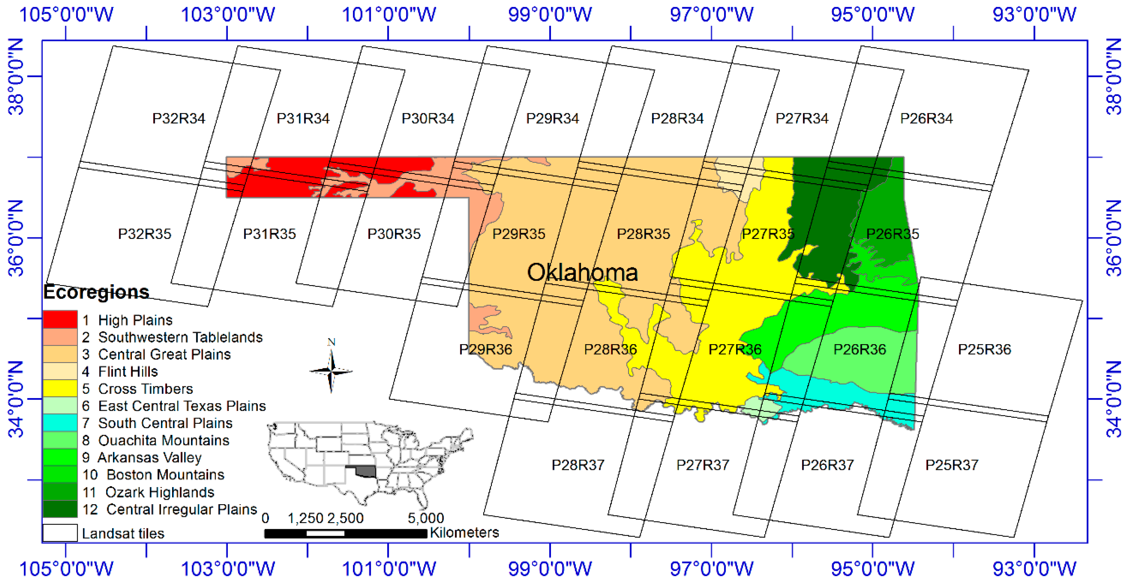
2.1. Study Area

The elevation increases from east to west in Oklahoma, ranging from 83 to 1517 m above sea level. The climate ranges from humid subtropical in the east to semi-arid in the west. Warm, moist air moving northward from the Gulf of Mexico exerts much influence over weather patterns in the state, particularly the southern and eastern parts. The annual average temperature decreases from the south (17.2 °C) to the north (12.8 °C), and the rainfall decreases from east (1320 mm) to the west (450 mm). Summers are long and usually very hot. There are nine different forested ecological system types and 164 tree species in Oklahoma [38].

2.2. Advanced Land Observation Satellite (ALOS) Phased Array Type L-Band Synthetic Aperture Radar (PALSAR) Images and Pre-Processing

The 25-m ALOS PALSAR Fine Beam Dual polarization (FBD) products from 2007 to 2010, generated with the selected images acquired between June and October [23], were downloaded from the Earth Observation Research Center, Japan Aerospace Exploration Agency (JAXA). The data are organized in 1 latitude degree by 1 longitude degree, about 4500 columns by 4500 rows. HH and HV gamma-naught, mask information (ocean flag, effective area, void area, layover and shadowing), local incidence angle, and total dates from the ALOS launch are included in the dataset. PALSAR HH and HV backscatter data were slope corrected and ortho-rectified with a geometric accuracy of about 12 m, using the 90-m Shuttle Radar Topography Mission (SRTM) Digital Elevation Model (DEM), before being radiometrically calibrated. The Digital Number (DN) values (amplitude values) were converted into gamma-naught backscattering coefficients in decibels ( γ ° ) using a calibration coefficient.
γ ° = 10 × log 10 DN 2 + CF
where CF is the absolute calibration factor of −83 [39]. PALSAR Difference and Ratio layers were calculated as follows:
Difference = HH HV
Ratio = HH HV
In order to match Landsat images at 30 m spatial resolution, we also resampled the 25 m PALSAR images (HH, HV, Difference and Ratio layers) to 30 m PALSAR images, using the nearest neighbor method. The resultant 30 m PALSAR images were then combined with Landsat images to compose a PALSAR/Landsat data cube.

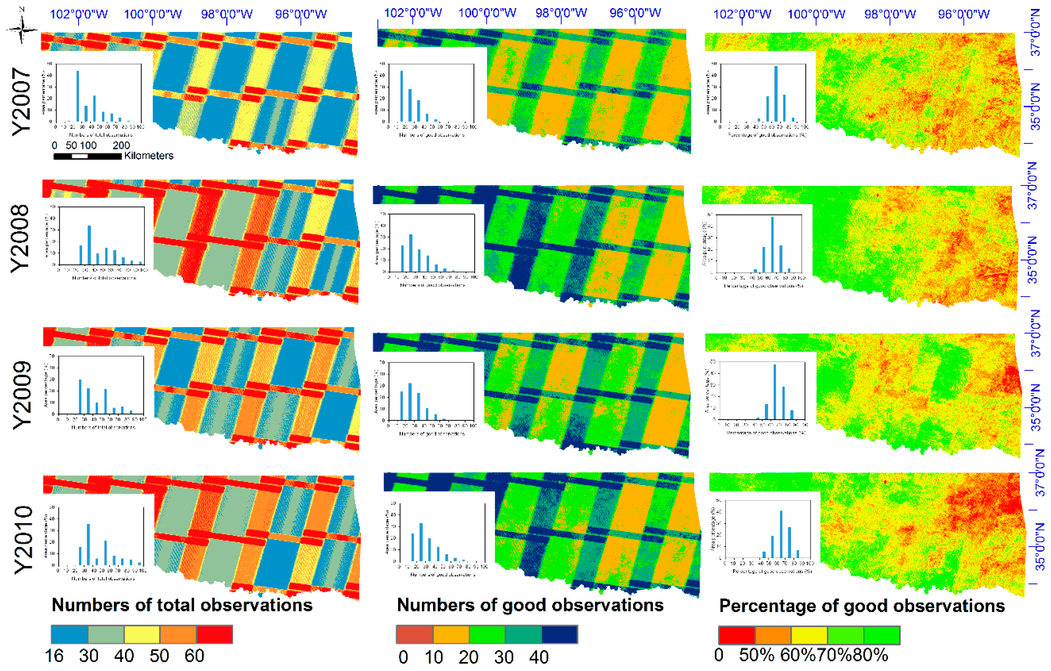
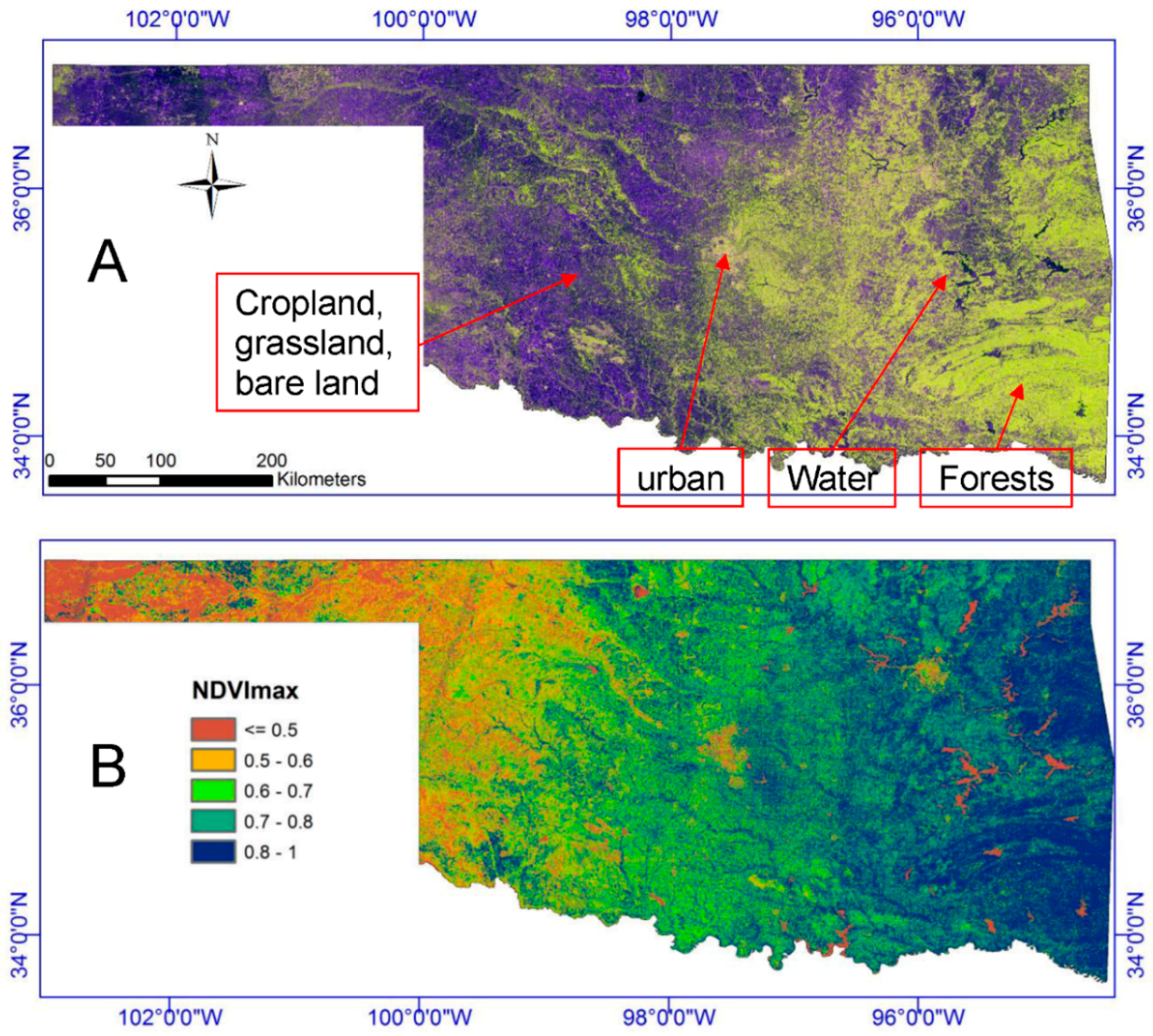
2.3. Landsat Images and Google Earth Engine

Google Earth Engine (GEE), an open and powerful platform for satellite imagery processing, was used for Landsat image processing. All the 2210 Landsat TM/ETM+ images in 23 tiles (path/row) were used in this study from 2007 to 2010 (Figure 1). Landsat has a 16-day revisit cycle, but the spatial overlaps among Landsat tiles provide additional observations for part of the images. The Landsat Ecosystem Disturbance Adaptive Processing System (LEDAPS) was used to convert the top of atmosphere reflectance (TOA) into surface reflectance (SR). A CFmask was applied to identify the bad observations (i.e., cloud, cloud shadow, snow) of Landsat images. Over 99.8% of pixels have more than 20 observations and ten good-quality observations in each year. The number of total observations and good-quality observations of Landsat images are relatively lower in 2007 than those in 2008, 2009 and 2010 (Figure 2). About 55.6%, 83.2%, 69.9% and 84.3% of pixels have more than 30 total observations in 2007, 2008, 2009 and 2010, respectively. About 55.9%, 77.0%, 74.8% and 76.0% of pixels have more than 20 good observations in 2007, 2008, 2009 and 2010, respectively. Most pixels have a percentage of good observations to total observations in the range of 50% to 80%.
The Normalized Difference Vegetation Index (NDVI) was calculated using Near Infrared band (0.85–0.88 µm) and Red band (0.64–0.67 µm) for all good-quality observations. The annual maximum NDVI (NDVImax) values were calculated for each year from 2007 to 2010.
NDVI = NIR Red NIR + Red

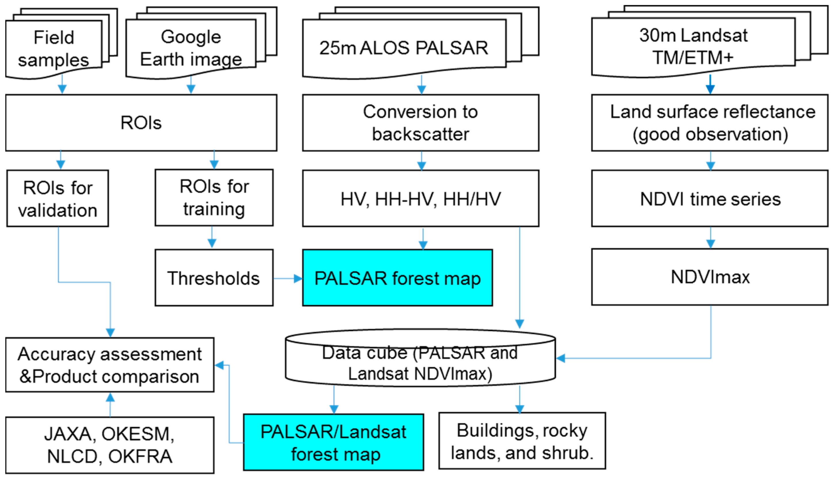
2.4. Algorithms for Mapping Forests through the Analyses of Landsat and PALSAR Images

Figure 3 illustrates a workflow that uses PALSAR and Landsat TM/ETM+ images to map forests (Figure 3). First, we use only PALSAR data (HV, Difference, and Ratio) to generate PALSAR-based forest maps. Second, we combine both PALSAR and Landsat NDVImax data into a data cube and generate PALSAR/Landsat forest maps, with an aim to reduce commission error in the forest maps.

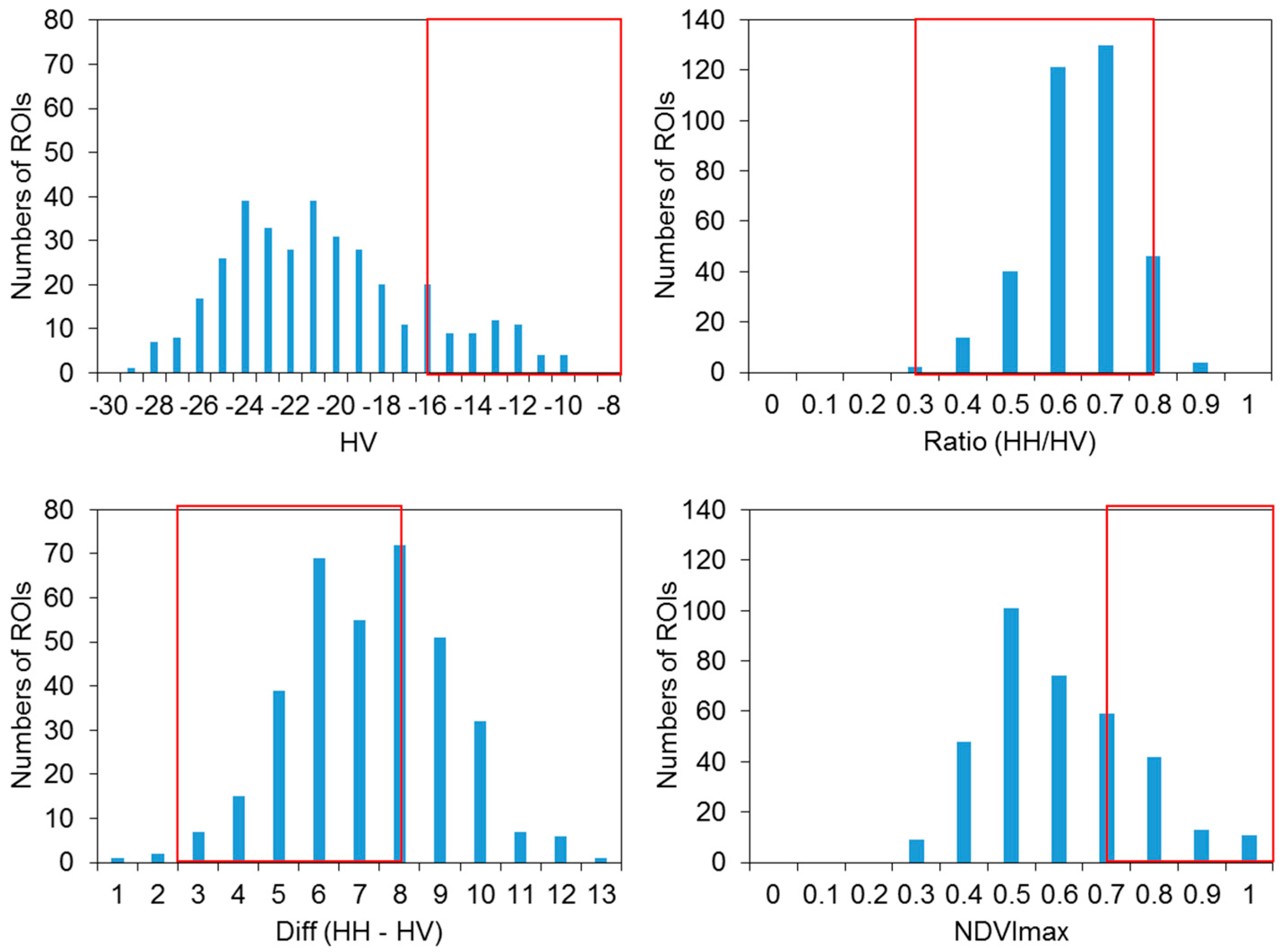
2.4.1. PALSAR-Based Forest Mapping Algorithm

As shown in Figure 4A, a false color composite of PALSAR data in Red (HH), Green (HV) and Blue (Difference) in 2010, the land cover types illustrate different color patterns. Forests present strong volume scattering signals in HV in green pixels; urban areas present strong volume scattering signals in both HH and HV in white pixels. The other land cover types without obvious structure properties (e.g., water bodies, agriculture land, and bare lands) show low volume scattering signals in dark color pixels.
According to the forest cover definition by the United Nations Food and Agriculture Organization (FAO), a forest is defined as a unit of land (>0.5 hectares) with tree crown cover of more than 10% and the minimum height of 5 m [40]. A histogram of typical land cover types (forests, croplands, urban, and others) in PALSAR HH, HV, Difference (HH-HV), and Ratio (HH/HV) in mainland Southeast Asia demonstrated the potential of a PALSAR dataset to identify these land cover types [26]. First, water has low values in both HH and HV and can easily be identified, since it reflects most of the backscatter through specular reflection. Second, L-band PALSAR has great penetration into forests, and its incident energy interacts with large trunks and branch components which causes substantial volume scattering. Forests have high values in both HH and HV, and low values in Difference (HH-HV); however, there is partial overlap with urban land cover types. Third, most croplands can also be identified, although they may partly overlap with water. Following the above analysis, a rule-based algorithm for forest mapping using 50 m PALSAR data was developed and assessed in China [41], Southeast Asia [26] and monsoon Asia [3]. In this study, we updated the PALSAR-based forest mapping algorithm, based on 25 m PALSAR data and large patches of training samples of typical land cover types (forests, croplands, urban, and others). The thresholds for the PALSAR-based forest mapping algorithm were updated as −16 < HV < −8 and 2 < Difference < 8 and 0.3 < Ratio < 0.85.

2.4.2. PALSAR/Landsat-Based Forest Mapping Algorithm

The PALSAR-based forest maps often have a commission error associated with some natural features (e.g., rocky lands) or manmade structures (e.g., urban, buildings), which tend to have lower NDVI. Forest has leaf area index greater values than 3 m2/m2 with NDVImax values greater than 0.7 [29,42,43], while rocky lands and urban areas have relatively low NDVImax values (Figure 4B). In order to differentiate forests from other natural or manmade land cover types, the PALSAR/Landsat-based forest mapping algorithm uses both Landsat NDVImax (>0.7) and the above-mentioned PALSAR data (Section 2.4.1), which helps reduce commission error of forest maps. In this study, the thresholds for the PALSAR/Landsat-based forest mapping algorithm were updated as −16 < HV < −8 and 2 < Difference < 8 and 0.3 < Ratio < 0.85 and NDVImax > 0.7 for the 30 m PALSAR/Landsat data cube.

2.4.3. Implementation of the Forest Mapping Algorithms

We ran the PALSAR-based forest mapping algorithm for the PALSAR data. For each pixel, we identified whether it was forested or non-forested by year (2007, 2008, 2009, and 2010). A temporal and logical consistency check was applied to reduce the noise or misclassification of this four-year forest/non-forest sequence [44], which has 16 different Forest (F)/Non-forest (N) permutations. Isolated states of forest or non-forest in a sequence is not reasonable and should be modified according to its temporal contexts. Therefore, the consistency filter was applied to the unreasonable permutations (NNFN→NNNN, NFNN→NNNN, FNFF→FFFF, and FFNF→FFFF), which reduced the misclassification. The reasonable (NNNN, NNNF, NNFF, NFFF, FNNN, FFNN, FFFN and FFFF) and random (NFNF, NFFN, FNNF and FNFN) permutations remained unchanged, as the consistency filter could not reduce the misclassification of random permutations, especially for short time permutations. We ran this procedure for all pixels and generated annual forest maps in 2007, 2008, 2009, and 2010. A median filter (5 × 5 pixels) was applied to exclude the isolated pixels and reduce the “salt and pepper” noise in the annual forest maps. The resultant 25-m forest maps were resampled to 30 m forest maps for comparison with other forest cover datasets, using the nearest neighbor resample method, here referred to as the PALSAR-based forest maps.
We also ran the PALSAR/Landsat-based forest mapping algorithm for the PALSAR and Landsat NDVImax data. The same procedures as described above were used to generate annual forest maps in 2007–2010, here referred to as the PALSAR/Landsat-based forest maps.

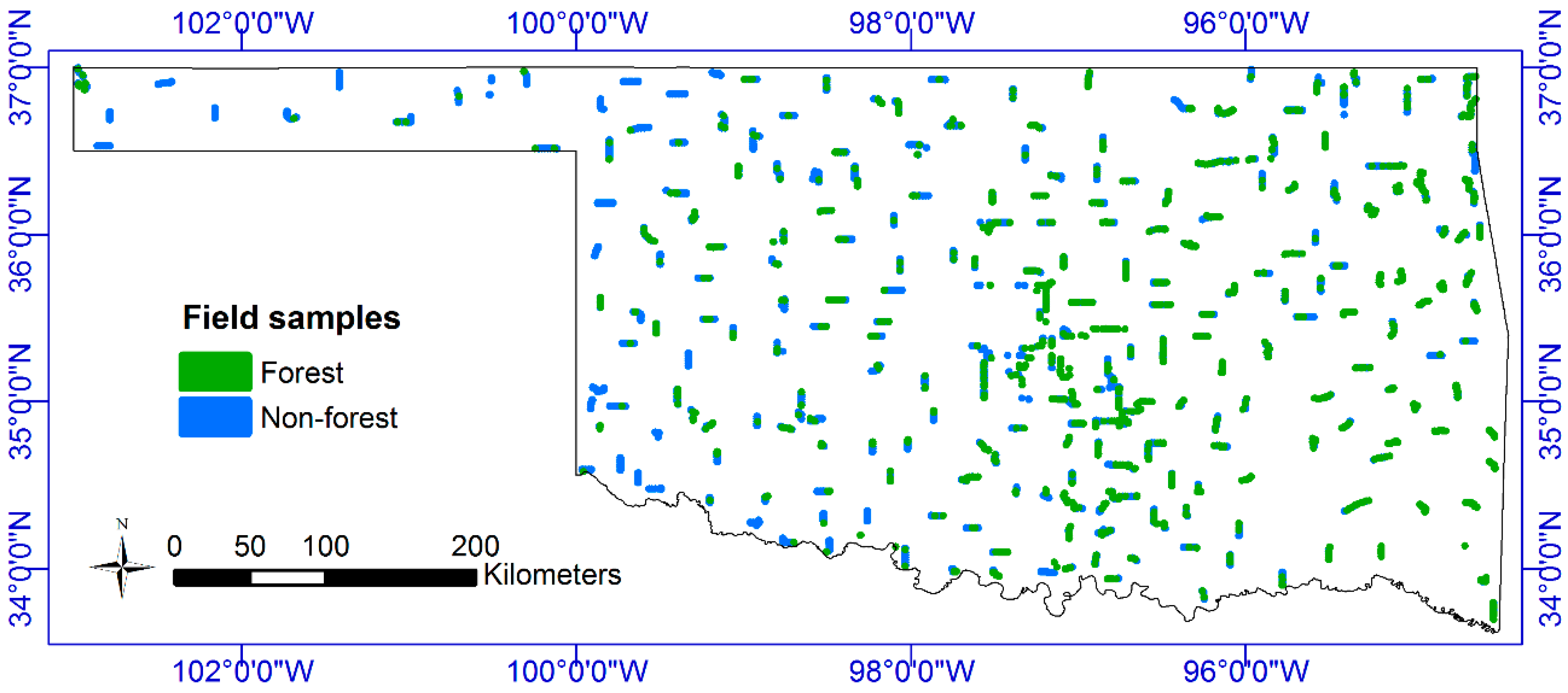
2.5. Validation Samples for Accuracy Assessment of PALSAR/Landsat Forest Maps

In an effort to generate the Oklahoma Ecological Systems Maps, extensive ground surveys were conducted to collect validation ground samples for 14 typical land cover types by the Oklahoma Biological Survey and the University of Oklahoma in 2012 and 2013. The collection of these ground samples included the following general procedure [38]:
Sample plots were selected and located either near a road or on accessible lands based on road or property access and variation in image signature or soil types. The locations were recorded in precise latitude and longitude coordinates, based on the use of a GPS receiver integrated with GIS software.
Samples along roads were collected at approximately 1.6 km intervals, often on both sides of the same road, starting from a random location. In addition, samples were collected at many stream/road crossings, and where uncommon plant communities were noted.
For data collected along the roads, all sample plots were located at least 60 m from the road within the center of a square with sides of at least 50 m, to help ensure that the footprint of a corresponding 30-m satellite pixel fell within a homogeneous land cover patch. Field survey table data and field photos were taken to record the detailed information of each sample plot.
The resultant in situ dataset was made available to us for evaluating the PALSAR- and PALSAR/Landsat-based forest maps. We made a 30 m buffer circle around each sample plot in the shapefile format in ArcGIS. Finally, we got 1496 and 2253 ground sample plots for forests and non-forest, respectively, for the accuracy assessment of the PALSAR/Landsat forest map in 2010 (Figure 5).

2.6. Multiple Forest Datasets for Spatial and Areal Comparison in Oklahoma in Circa 2010

To analyze the consistency and uncertainty of the available forest maps at relatively high spatial resolutions in Oklahoma, we carried out the area and spatial comparison between the 30-m PALSAR/Landsat forest map in 2010 and the 25-m JAXA forest/non-forest map (JAXA F/NF) [23], 30-m National Land Cover Database 2011 (NLCD2011) [14,15], 10-m Oklahoma Ecological Systems Map (OKESM) [38], and the Oklahoma Forest Resource Assessment 2010 (OKFRA2010) [45]. The 25 m JAXA FNF was resampled into a 30 m binary forest/non-forest map using nearest interpolation algorithm. The 10 m OKSEM was aggregated into 30 m forest map under the original forest definition. Table 1 provides the brief introduction of these forest products in Oklahoma.

3. Results

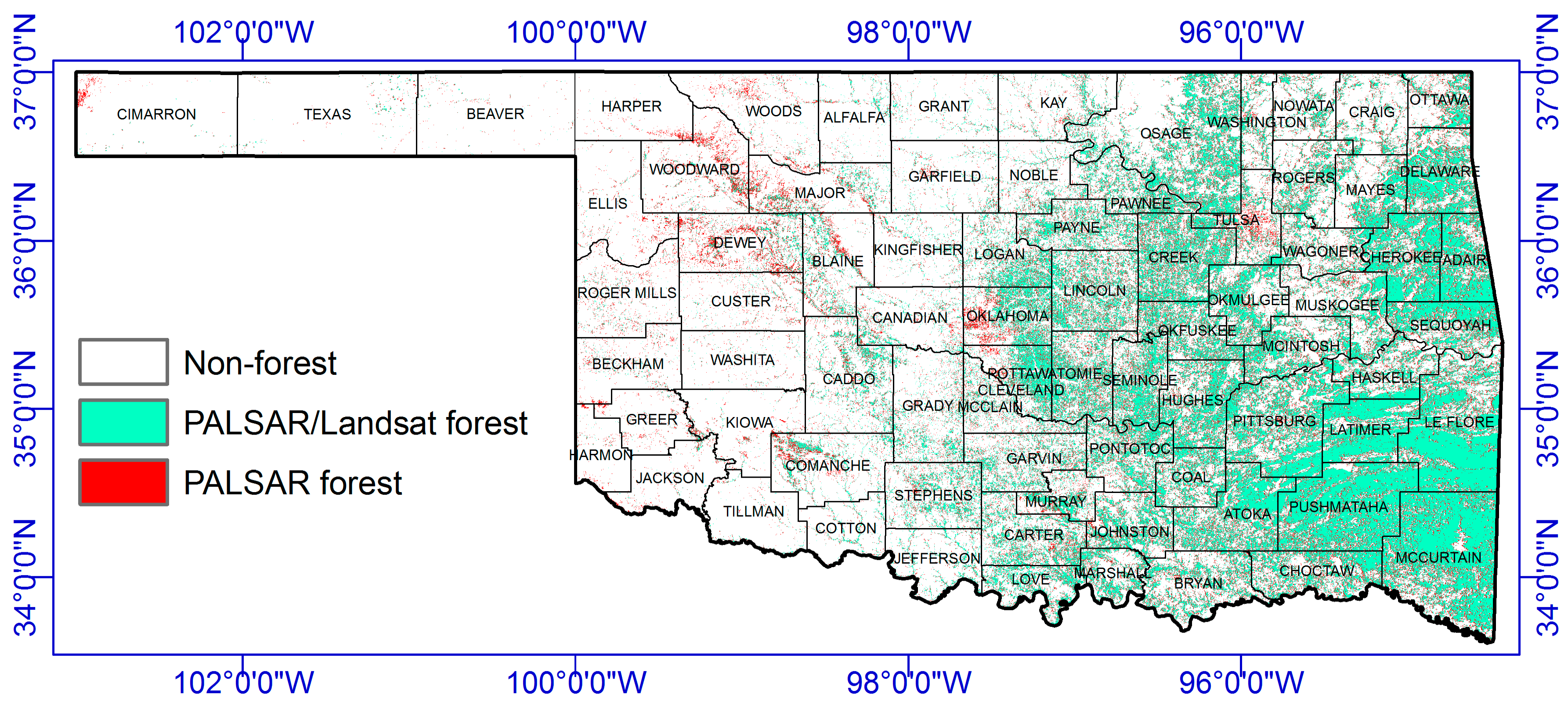
3.1. The PALSAR/Landsat Forest Map in Oklahoma in 2010

The spatial distribution of PALSAR/Landsat forest in 2010 showed a relatively good spatial match with climate conditions (Figure 6). For example, the climate in eastern and central Oklahoma is warm and humid, and subsequently large areas of forests were mapped; however, in western Oklahoma where it is warm and dry, only a small area of forest is distributed. As shown in the confusion matrix generated by the ground samples of forests and non-forest (Table 2), the overall accuracy and Kappa coefficient of the PALSAR/Landsat-based forest map in 2010 were about 88.2% and 0.75; the producer and user accuracies were about 75.7% and 93.4%, respectively. Due to limited human and financial resources, ground samples collected in 2012 and 2013 were used to assess the accuracy of the PALSAR/Landsat forest map in 2010, which would include some uncertainty caused by forest change within this three-year interval. It was estimated that the total forest area from the PALSAR/Landsat forest map in 2010 was 40,419 km2, about 22% of the entire state area.

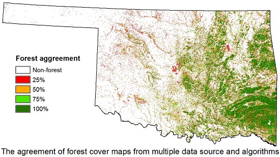
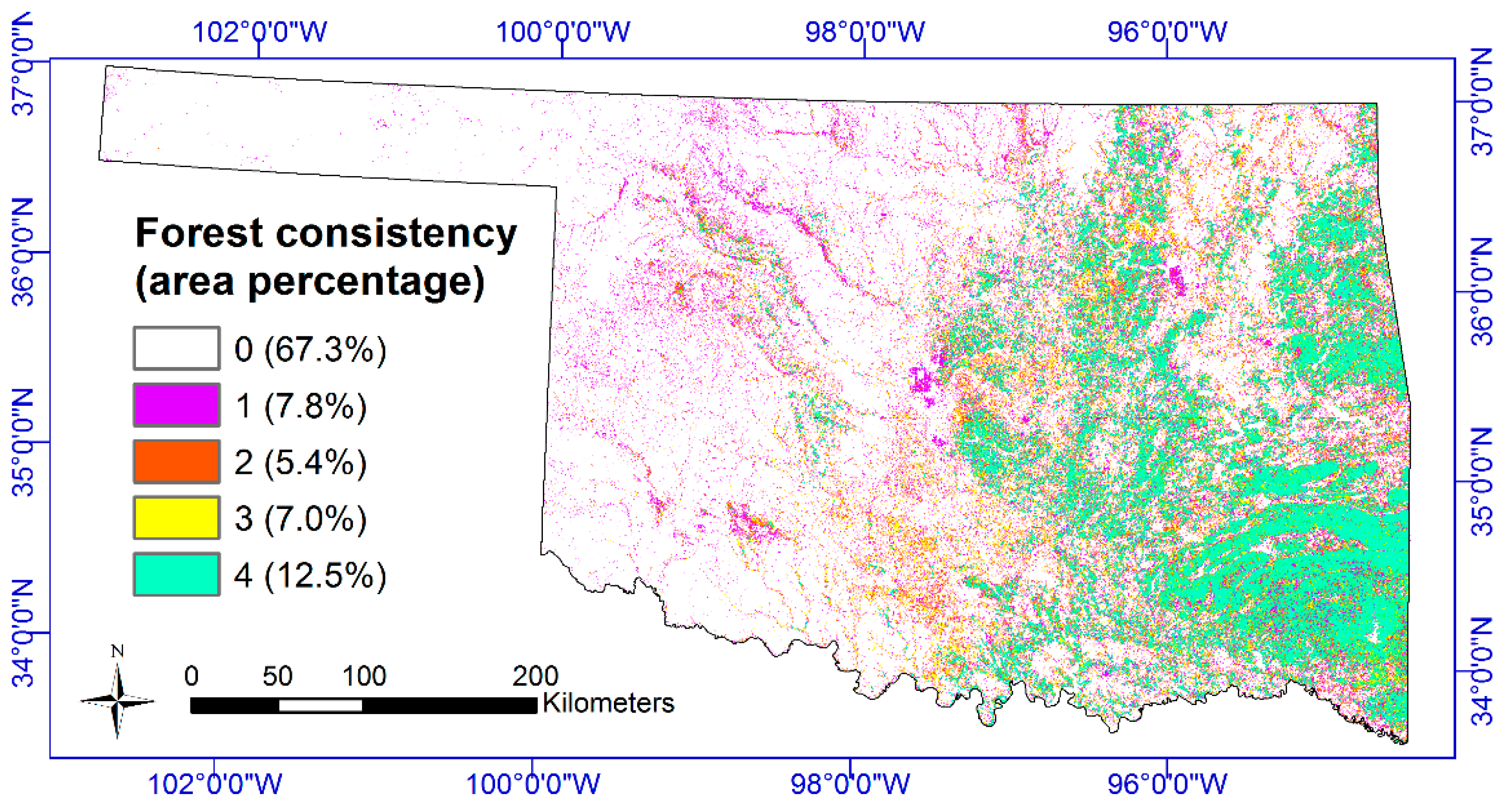
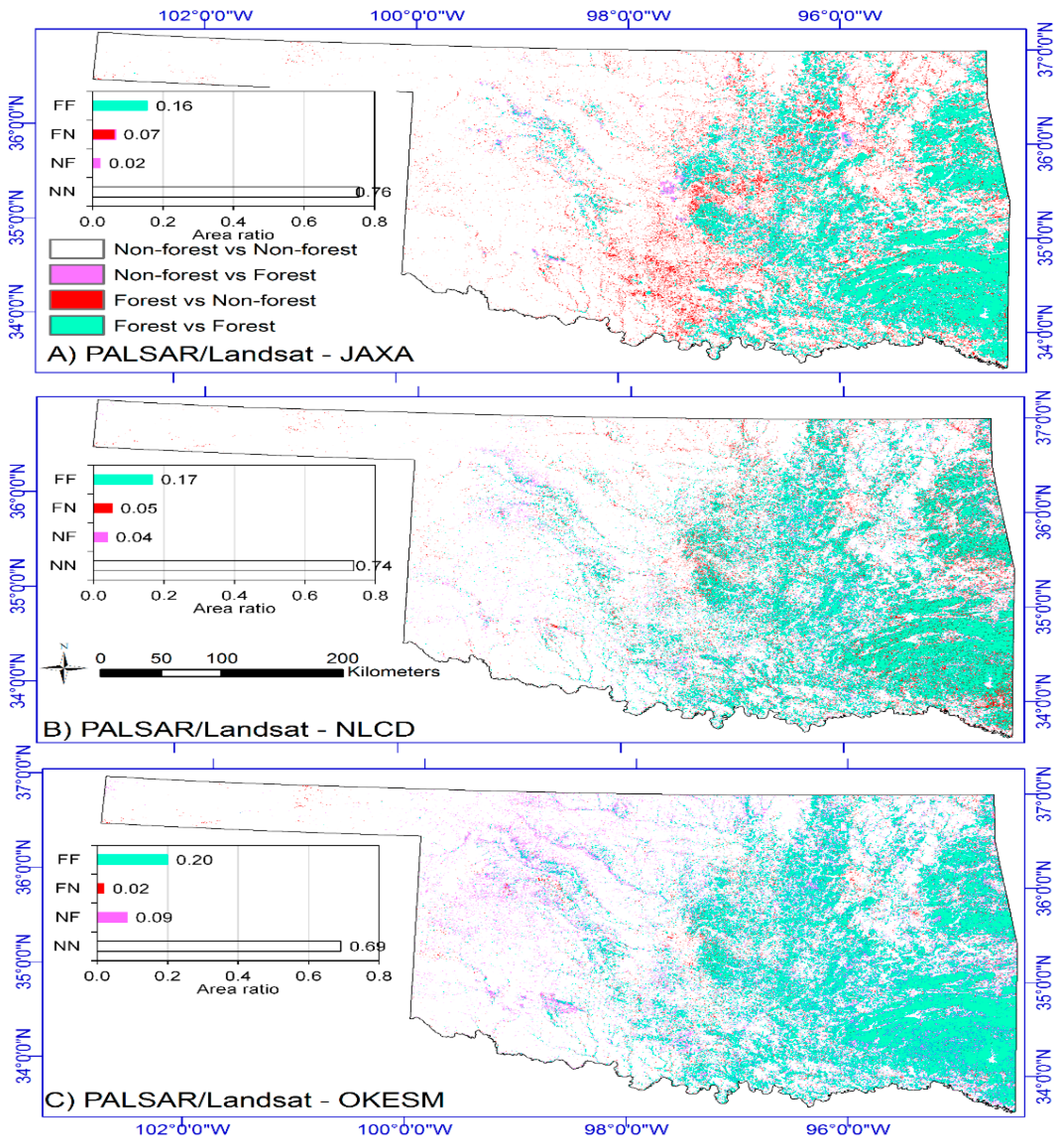
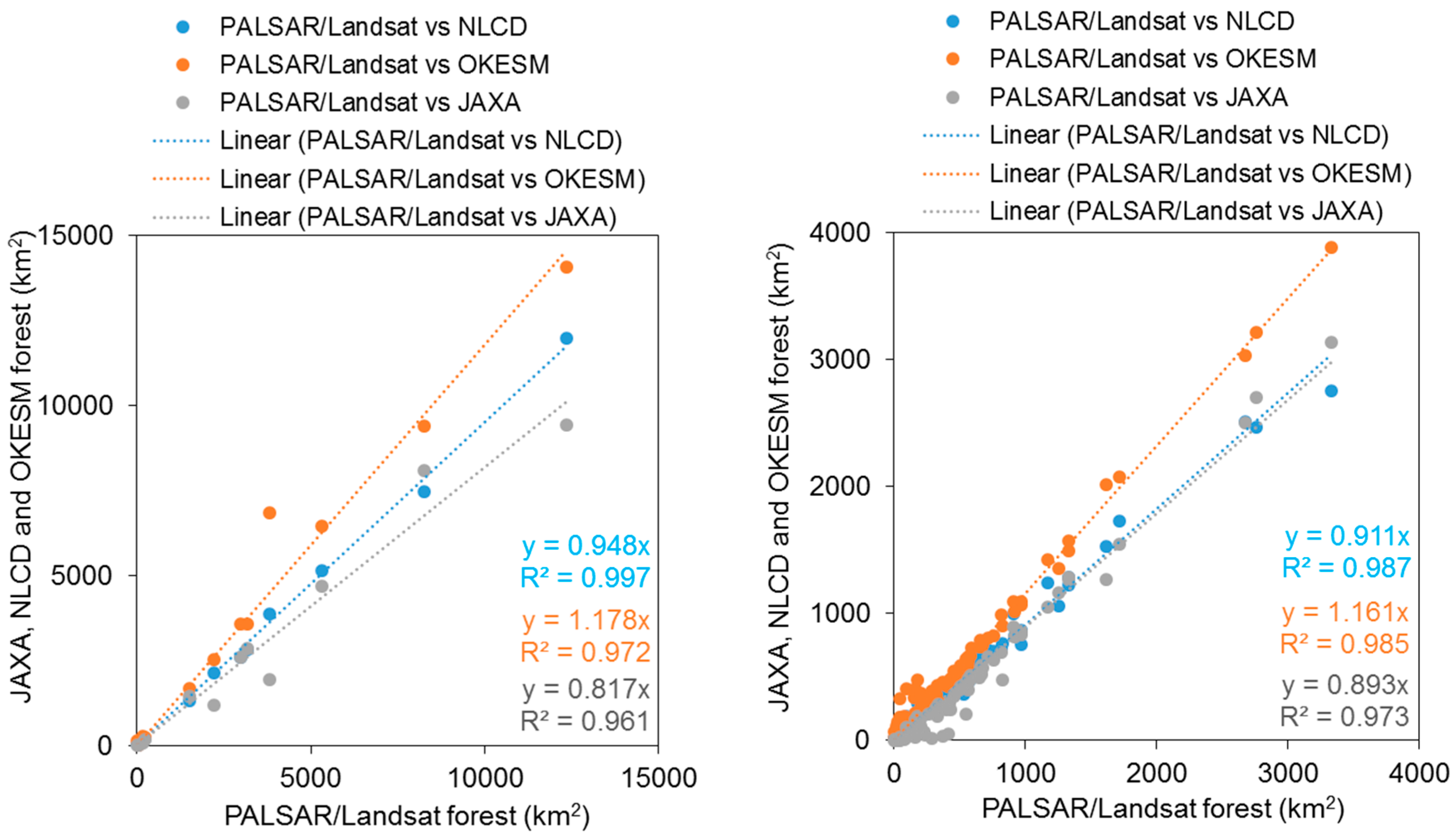
3.2. Spatial and Areal Comparison Among Multiple Forest Datasets Circa 2010

At the pixel scale, these forest maps showed relatively good consistency in the regions with high forest coverage (e.g., the southeast of Oklahoma) and large uncertainties in the regions with low forest coverage (e.g., the west of Oklahoma) (Figure 7). Out of the entire state area, about 12.5% and 67.3% of pixels were identified as consistent forest and non-forest by those forest maps. In detail, about 16%, 17% and 20% of the total pixels were identified as consistent forest between PALSAR/Landsat forest map and JAXA forest map, NLCD2011 forest map and OKESM forest map, as well as 76%, 74% and 69% of consistent non-forest pixels, respectively (Figure 8). Compared with the PALSAR/Landsat forest map, JAXA forest map clearly underestimated forests in the western and central parts of Oklahoma by about 7% of the total pixels (Figure 9) and included obvious commission errors from urban areas (Figure 8A). In southeast and central Oklahoma, the NLCD2011 forest map underestimated the forested area by 5% of the total study area, and it overestimated forest area by about 4% of the total study area in the west (Figure 8B and Figure 9). The OKESM forest map overestimated forest area about 9% of the total study area, including shrublands in both western and southeastern Oklahoma (Figure 8C and Figure 9).
At the state scale, the total forested area from the PALSAR/Landsat-based forest map in 2010 was estimated to be 40,419 km2, which was close to the official forest statistics (40,468 km2) from the OKFRA but higher than the estimates from the JAXA forest map (32,403 km2) and NLCD2011 forest map (37,628 km2) and lower than the estimate from the OKESM forest map (48,665 km2). The forested areas from the nine ecoregions and 77 counties had significant linear relationships among the datasets (Figure 10). The OKESM tended to have higher forested areas, while JAXA and NLCD2011 tended to have lower forest areas when compared with the forest area estimates from the PALSAR/Landsat forest map in 2010 (Figure 10).

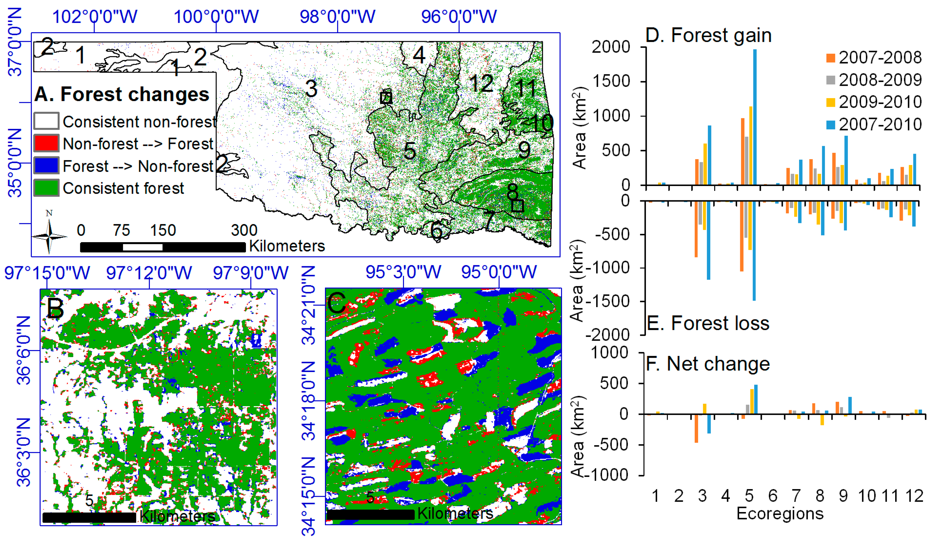
3.3. Spatial and Areal Changes of Forests from 2007 to 2010

We overlaid the PALSAR/Landsat forest maps and identified those pixels that remained as forest over the four-year period and those pixels experienced forest changes in Oklahoma from 2007 to 2010 (Figure 11). Limited to human and financial resources, we analyzed forested area change based on the map-based forested areas instead of sample-based unbiased forested areas. Generally, total forested area was relatively stable in Oklahoma from 2007 to 2010, with a slight increase from 39,465 km2 in 2007 to 40,419 km2 in 2010 (~2.4% increase). The annual average forest cover loss rate was about 1572 km2/year, and the annual average forest cover gain rate was about 1800 km2/year from 2007 to 2010, respectively. Geographically, there were two regions with relatively high forest cover changes in Oklahoma. The Cross Timbers ecoregion showed the largest forest cover gain (about 1969 km2) and loss (1486 km2) during 2007–2010, followed by the southeastern region (South Central Plains, Ouachita Mountains, and Arkansas Valley ecoregions) of Oklahoma with large areas of pine plantations (Figure 11). According to the Oklahoma Forest Resource Assessment, several possible causes are responsible for forest cover change [45]. The relatively low price of pulpwood and the declining forest industry in Oklahoma left landowners investing little management in forests. The industry’s standard logging and planting cycles are primary causes for the forest cover loss and gain, which is especially apparent in the pine plantation region of southeast Oklahoma. Furthermore, under the pressure of urbanization and landowner income, some forests were developed or converted into pasture.

4. Discussion

4.1. Integration of PALSAR and Landsat Imagery for Forest Mapping

We applied a pixel-based algorithm to generate annual forest distribution maps at the spatial resolution of 30 m in Oklahoma from 2007 to 2010, through the integration and analysis of PALSAR and Landsat TM/ETM+ imagery. The proposed algorithm combined the advantages of forest structure information from PALSAR imagery and greenness information from Landsat NDVImax. Compared with the other forest data products at similar spatial resolution, the PALSAR/Landsat forest maps have several advantages as follows. First, the PALSAR/Landsat forest maps had limited commission error from shrubs. Distinguishing forests from shrublands is challenging in the sub-humid and semi-arid regions, as some shrubs have similar greenness and phenology features with forest trees [28,29]. The heights of shrublands were lower than those of forests, which may be distinguishable in PALSAR HV. Based on the ground samples of shrublands, we analyzed the confusion condition between forests and shrublands. The PALSAR forest map excluded 85.7% of shrublands and Landsat NDVImax 74.2% of shrublands (Figure 12). In total, about 92.4% of shrublands were excluded from the PALSAR/Landsat forest map. Second, Landsat NDVImax refined the PALSAR forest maps and reduced the commission errors. In Figure 6, the PALSAR/Landsat forest and the PALSAR forest showed the relatively large difference in the land cover of western Oklahoma and urban areas. The inclusion of Landsat NDVImax could exclude the commission errors from shrublands and urban areas in the PALSAR forest map (Figure 13). The areas of the PALSAR forest maps were about 43,787 km2, 42,820 km2, 44,579 km2 and 43,965 km2 from 2007 to 2010, respectively. After including Landsat NDVImax, the areas of the PALSAR/Landsat forest maps were about 39,465 km2, 39,394 km2, 39,731 km2 and 40,149 km2, respectively, about 10% (~4000 km2) of shrub, buildings, and rocky land were reduced.

4.2. Reasons for the Differences between the PALSAR/Landsat Forest Map and Other Forest Data Products

There are several reasons to explain the differences between the PALSAR/Landsat forest map and other forest data products in this study:
The first reason is the definition of forests. A major difference in the spatial distribution of forest maps is located in the regions with low forest coverage, which was thought to be mainly contributed by the definition of forests [2]. The PALSAR/Landsat forests and the JAXA forests both use the FAO forest definition: forest canopy coverage >10% and tree heights >5 m with a minimum area >0.5 hectares. The forests from OKFRA and NLCD2011 are defined as land cover with >20% forest canopy coverage and trees >5 m in height. Compared with the PALSAR/Landsat forest map, NLCD2011 has a smaller area of forest (37,628 km2), while OKFRA has a larger area of forest (40,468 km2), which may be attributed to the refining process based on the areal images. Forest in the OKESM is defined as having a land cover of >25% forest canopy coverage and tree heights >4 m, which has 8516 km2 more forest area (21.2%) than that of the PALSAR/Landsat forest map.
The second reason is the data sources. The JAXA FNF was purely generated based on the strong PALSAR backscatter of forest in HV gamma-naught, which included commission errors from urban-rural areas and sparsely vegetated land [23]. Two or three cloud-free Landsat images, selected from multiple years, are the major data source to generate the NLCD, OKESM and OKFRA products, and the forests in these products were easily confused with other land cover types; e.g., shrublands or recent forest openings due to logging activities and natural disturbances. The PALSAR/Landsat forest maps were produced by the integration of ALOS PALSAR and Landsat images, which contains more information to reduce commission errors in the forest maps. In this study, the data sources for several forest products were in different years or a collection of multiple years. This would cause certain underestimations or overestimations of the area and spatial distribution of forests and is not preferred for mapping fast-changing forests, like those of southeast Oklahoma.
The third reason is the algorithms of forest mapping. All four forest mapping products were generated by the decision tree algorithms with different pre-processing and post-processing techniques (Table 1). Different input datasets and thresholds derived from training samples resulted in different forest maps. For example, the JAXA FNF map was produced based on the PALSAR HV threshold (>−14.2 DB) [23], which was larger than that of the PALSAR/Landsat forest mapping algorithm in this study (HV > −16 DB). Thus, the JAXA FNF map tends to underestimate the forest distribution, approximately 7746 km2 (~23.9%) smaller than the PALSAR/Landsat forest map and includes commission error from urban areas (Figure 8A and Figure 10). The NLCD2011 was updated based on the NLCD2006 through the interpretation of two pairs of cloud-free Landsat images and several ancillary datasets, as well as substantial post-processing [15], which is relatively complex. The OKFRA forest dataset was from Oklahoma Forestry Services and derived from Landsat images.
The fourth reason is the spatial extent of forest products. JAXA and NLCD2011 provide global and national forest maps, respectively, while OKESM and OKFRA2010 are statewide forest products for Oklahoma. Although the PALSAR/Landsat forest product uses the rules collected from large areas of training samples and a knowledge-based threshold and could be used for global forest mapping, its application is currently only in Oklahoma. It is expected that statewide forest products usually have high accuracy, and national/global forest products usually have good spatial consistency, though relatively low accuracy of large spatial coverage rendering landscape conditions more complicated.

4.3. Applications of the PALSAR/Landsat Forest Maps in the Forest Management in Oklahoma

It is challenging to manage the forest resources in Oklahoma, as the area and spatial distribution of forest are being affected by multiple factors, including changing forest markets, climate, and landowner income [45]. Lots of forests are being clear-cut and used for pulpwood production. Therefore, timely and fine spatial resolution forest maps are critically needed for forest management and policy development [46].
The integration of PALSAR and Landsat images provided complementary information for other datasets, including Forest Inventory and Analysis (FIA) and airborne LiDAR, to estimate and track forests. FIA collects many informative inventory data (e.g., tree species, size and condition of trees, and forest land ownership) from a grid of permanent plots established about three miles apart in Oklahoma about every five years. LiDAR can capture the structure information of forests and has a very good relationship with forest biomass [47]. Both FIA and LiDAR data are expensive and have low observation frequency, which is not preferred for mapping fast forest changes in relatively large areas. As cloud and cloud shadows restrict data availability and utility, Landsat images are often selected from multiple years to increase the number of good-quality observations and to produce land cover maps, including forest maps at large scales [12,15,48], which fails to detect forest changes and could introduce large uncertainties in the estimation of forest fragmentation, forest biomass and carbon cycling [2,46]. Based on the resultant PALSAR/Landsat forest maps, extensive forest cover loss and gain were identified in Oklahoma from 2007 to 2010, especially in the southeastern region of Oklahoma.
The areas of forests have increased in central and western Oklahoma, where rangeland is predominant and vulnerable to woody encroachment. The woody plant encroachment into grasslands has considerable effects on the ecosystem, such as (1) increase in soil C and N [49]; (2) decline in grass cover and soil pH; (3) significant declines in species richness [50]; (4) altered carbon balance [51]; (5) changes in the ecohydrological process [52]; and (6) a reduction in livestock production in a highly productive area [53]. The PALSAR/Landsat forest maps could provide the forest extent and its spatio-temporal changes to policy makers for identification and management of the woody encroachment in the region.

5. Conclusions

In sub-humid and semi-arid regions, relatively large uncertainties and low temporal precision occur when one estimates forest distribution based on either synthetic aperture radar (SAR) or optical remote sensing images alone. In this study, taking Oklahoma in the central United States as an example, we introduced a straightforward and robust rule-based algorithm for forest mapping using Advanced Land Observation Satellite (ALOS) Phased Array type L-band Synthetic Aperture Radar (PALSAR) Fine Beam Dual polarization (FBD) mosaic images and the Landsat annual maximum of Normalized Difference Vegetation Index (NDVImax). The PALSAR/Landsat forest map in 2010 reached a relatively high overall accuracy and showed improvements against selected forest maps. The forested areas tended to increase about 684 km2 from 2007 to 2010. The resultant PALSAR/Landsat forest maps would provide the timely and accurate data source for forest management and policy development in this sub-humid to semi-arid climate transition zone with the complex landscape.

Acknowledgments

This study was supported in part by research grants from the National Institute of Food and Agriculture, U.S. Department of Agriculture (2013-69002), the National Science Foundation (NSF) EPSCoR program (OIA-1301789), and the Department of the Interior, United States Geological Survey to AmericaView (G14AP00002). We thank Sarah Xiao at Yale University and the writing center at the University of Oklahoma for English editing of the manuscript.

Author Contributions

X.X. and Y.Q. conceived and designed this study; Y.Q. and J.W. performed data analysis and forest mapping; K.E., B.H., D.H. and T.F. collected and organized ground reference; all authors wrote the paper.

Conflicts of Interest

The authors declare no conflict of interest.

References

  1. United Nations Convention to Combat Desertification. Redd+ and desertification. Available online: http://www.unccd.int/Lists/SiteDocumentLibrary/Publications/Factsheet%207%20redd.ENGweb.pdf (accessed on 16 June 2011).
  2. Sexton, J.O.; Noojipady, P.; Song, X.-P.; Feng, M.; Song, D.-X.; Kim, D.-H.; Anand, A.; Huang, C.; Channan, S.; Pimm, S.L.; et al. Conservation policy and the measurement of forests. Nat. Clim. Chang. 2015, 6, 192–196. [Google Scholar] [CrossRef]
  3. Qin, Y.; Xiao, X.; Dong, J.; Zhang, G.; Roy, P.S.; Joshi, P.K.; Gilani, H.; Murthy, M.S.; Jin, C.; Wang, J.; et al. Mapping forests in monsoon Asia with ALOS PALSAR 50-m mosaic images and MODIS imagery in 2010. Sci. Rep. 2016, 6, 20880. [Google Scholar] [CrossRef] [PubMed]
  4. Van der Werf, G.R.; Morton, D.C.; DeFries, R.S.; Olivier, J.G.J.; Kasibhatla, P.S.; Jackson, R.B.; Collatz, G.J.; Randerson, J.T. CO2 emissions from forest loss. Nat. Geosci. 2009, 2, 737–738. [Google Scholar] [CrossRef]
  5. Houghton, R.A.; Goetz, S.J. New satellites help quantify carbon sources and sinks. Eos Trans. Am. Geophys. Union 2008, 89, 417–418. [Google Scholar] [CrossRef]
  6. Hansen, M.C.; DeFries, R.S. Detecting long-term global forest change using continuous fields of tree-cover maps from 8-km advanced very high resolution radiometer (AVHRR) data for the years 1982–99. Ecosystems 2004, 7, 695–716. [Google Scholar] [CrossRef]
  7. Loveland, T.R.; Reed, B.C.; Brown, J.F.; Ohlen, D.O.; Zhu, Z.; Yang, L.; Merchant, J.W. Development of a global land cover characteristics database and IGBP DISCover from 1 km AVHRR data. Int. J. Remote Sens. 2000, 21, 1303–1330. [Google Scholar] [CrossRef]
  8. Hansen, M.C.; DeFries, R.S.; Townshend, J.R.G.; Carroll, M.; Dimiceli, C.; Sohlberg, R.A. Global percent tree cover at a spatial resolution of 500 meters: First results of the MODIS vegetation continuous fields algorithm. Earth Interact. 2003, 7, 1–15. [Google Scholar] [CrossRef]
  9. Hansen, M.C.; Stehman, S.V.; Potapov, P.V.; Loveland, T.R.; Townshend, J.R.G.; DeFries, R.S.; Pittman, K.W.; Arunarwati, B.; Stolle, F.; Steininger, M.K.; et al. Humid tropical forest clearing from 2000 to 2005 quantified by using multitemporal and multiresolution remotely sensed data. Proc. Natl. Acad. Sci. USA 2008, 105, 9439–9444. [Google Scholar] [CrossRef] [PubMed]
  10. Friedl, M.A.; Sulla-Menashe, D.; Tan, B.; Schneider, A.; Ramankutty, N.; Sibley, A.; Huang, X.M. MODIS Collection 5 global land cover: Algorithm refinements and characterization of new datasets. Remote Sens. Environ. 2010, 114, 168–182. [Google Scholar] [CrossRef]
  11. Hansen, M.C.; Potapov, P.V.; Moore, R.; Hancher, M.; Turubanova, S.A.; Tyukavina, A.; Thau, D.; Stehman, S.V.; Goetz, S.J.; Loveland, T.R.; et al. High-resolution global maps of 21st-century forest cover change. Science 2013, 342, 850–853. [Google Scholar] [CrossRef] [PubMed]
  12. Kim, D.H.; Sexton, J.O.; Noojipady, P.; Huang, C.Q.; Anand, A.; Channan, S.; Feng, M.; Townshend, J.R. Global, Landsat-based forest-cover change from 1990 to 2000. Remote Sens. Environ. 2014, 155, 178–193. [Google Scholar] [CrossRef]
  13. Townshend, J.R.; Masek, J.G.; Huang, C.Q.; Vermote, E.F.; Gao, F.; Channan, S.; Sexton, J.O.; Feng, M.; Narasimhan, R.; Kim, D.; et al. Global characterization and monitoring of forest cover using landsat data: Opportunities and challenges. Int. J. Digit. Earth 2012, 5, 373–397. [Google Scholar] [CrossRef]
  14. Homer, C.; Dewitz, J.; Yang, L.M.; Jin, S.; Danielson, P.; Xian, G.; Coulston, J.; Herold, N.; Wickham, J.; Megown, K. Completion of the 2011 national land cover database for the conterminous united states-representing a decade of land cover change information. Photogramm. Eng. Remote Sens. 2015, 81, 345–354. [Google Scholar]
  15. Jin, S.M.; Yang, L.M.; Danielson, P.; Homer, C.; Fry, J.; Xian, G. A comprehensive change detection method for updating the National Land Cover Database to circa 2011. Remote Sens. Environ. 2013, 132, 159–175. [Google Scholar] [CrossRef]
  16. Kovacs, J.M.; Lu, X.X.; Flores-Verdugo, F.; Zhang, C.; de Santiago, F.F.; Jiao, X. Applications of ALOS PALSAR for monitoring biophysical parameters of a degraded black mangrove (Avicennia germinans) forest. ISPRS J. Photogramm. Renmote Sens. 2013, 82, 102–111. [Google Scholar] [CrossRef]
  17. Ni, W.J.; Sun, G.Q.; Guo, Z.F.; Zhang, Z.Y.; He, Y.T.; Huang, W.L. Retrieval of forest biomass from ALOS PALSAR data using a lookup table method. IEEE J. Sel. Top. Appl. Earth Obs. Remote Sens. 2013, 6, 875–886. [Google Scholar] [CrossRef]
  18. Lucas, R.M.; Cronin, N.; Lee, A.; Moghaddam, M.; Witte, C.; Tickle, P. Empirical relationships between AIRSAR backscatter and LIDAR-derived forest biomass, Queensland, Australia. Remote Sens. Environ. 2006, 100, 407–425. [Google Scholar] [CrossRef]
  19. Shimada, M. Long-term stability of L-band normalized radar cross section of Amazon rainforest using the JERS-1 SAR. Can. J. Remote Sens. 2005, 31, 132–137. [Google Scholar] [CrossRef]
  20. Sgrenzaroli, M.; De Grandi, G.F.; Eva, H.; Achard, F. Tropical forest cover monitoring: Estimates from the GRFM JERS-1 radar mosaics using wavelet zooming techniques and validation. Int. J. Remote Sens. 2002, 23, 1329–1355. [Google Scholar] [CrossRef]
  21. Simard, M.; Saatchi, S.S.; De Grandi, G. The use of decision tree and multiscale texture for classification of JERS-1 SAR data over tropical forest. IEEE Trans. Geosci. Remote Sens. 2000, 38, 2310–2321. [Google Scholar] [CrossRef]
  22. Saatchi, S.S.; Nelson, B.; Podest, E.; Holt, J. Mapping land cover types in the Amazon basin using 1 km JERS-1 mosaic. Int. J. Remote Sens. 2000, 21, 1201–1234. [Google Scholar] [CrossRef]
  23. Shimada, M.; Itoh, T.; Motooka, T.; Watanabe, M.; Shiraishi, T.; Thapa, R.; Lucas, R. New global forest/non-forest maps from ALOS PALSAR data (2007–2010). Remote Sens. Environ. 2014, 155, 13–31. [Google Scholar] [CrossRef]
  24. Motohka, T.; Shimada, M.; Uryu, Y.; Setiabudi, B. Using time series PALSAR gamma nought mosaics for automatic detection of tropical deforestation: A test study in Riau, Indonesia. Remote Sens. Environ. 2014, 155, 79–88. [Google Scholar] [CrossRef]
  25. Pantze, A.; Santoro, M.; Fransson, J.E.S. Change detection of boreal forest using bi-temporal ALOS PALSAR backscatter data. Remote Sens. Environ. 2014, 155, 120–128. [Google Scholar] [CrossRef]
  26. Dong, J.W.; Xiao, X.M.; Sheldon, S.; Biradar, C.; Duong, N.D.; Hazarika, M. A comparison of forest cover maps in mainland southeast Asia from multiple sources: PALSAR, MERIS, MODIS and FRA. Remote Sens. Environ. 2012, 127, 60–73. [Google Scholar] [CrossRef]
  27. Ranson, K.J.; Sun, G.Q. An evaluation of AIRSAR and SIR-C/X-SAR images for mapping northern forest attributes in Maine, USA. Remote Sens. Environ. 1997, 59, 203–222. [Google Scholar] [CrossRef]
  28. Asner, G.P. Cloud cover in Landsat observations of the Brazilian Amazon. Int. J. Remote. Sens. 2001, 22, 3855–3862. [Google Scholar] [CrossRef]
  29. Gamon, J.A.; Field, C.B.; Goulden, M.L.; Griffin, K.L.; Hartley, A.E.; Joel, G.; Penuelas, J.; Valentini, R. Relationships between NDVI, canopy structure, and photosynthesis in 3 Californian vegetation types. Ecol. Appl. 1995, 5, 28–41. [Google Scholar] [CrossRef]
  30. Yan, E.P.; Wang, G.X.; Lin, H.; Xia, C.Z.; Sun, H. Phenology-based classification of vegetation cover types in Northeast China using MODIS NDVI and EVI time series. Int. J. Remote Sens. 2015, 36, 489–512. [Google Scholar] [CrossRef]
  31. Ranson, K.J.; Kovacs, K.; Sun, G.; Kharuk, V.I. Disturbance recognition in the boreal forest using radar and Landsat-7. Can. J. Remote Sens. 2003, 29, 271–285. [Google Scholar] [CrossRef]
  32. Khazendar, A.; Rignot, E.; Larour, E. Larsen B Ice Shelf rheology preceding its disintegration inferred by a control method. Geophys. Res. Lett. 2007, 34, 1–6. [Google Scholar] [CrossRef]
  33. Ban, Y.F. Synergy of multitemporal ERS-1 SAR and Landsat TM data for classification of agricultural crops. Can. J. Remote Sens. 2003, 29, 518–526. [Google Scholar] [CrossRef]
  34. Haack, B.N.; Solomon, E.K.; Bechdol, M.A.; Herold, N.D. Radar and optical data comparison/integration for urban delineation: A case study. Photogramm. Eng. Remote Sens. 2002, 68, 1289–1296. [Google Scholar]
  35. Reiche, J.; Verbesselt, J.; Hoekman, D.; Herold, M. Fusing Landsat and SAR time series to detect deforestation in the tropics. Remote Sens. Environ. 2015, 156, 276–293. [Google Scholar] [CrossRef]
  36. Lehmann, E.A.; Caccetta, P.; Lowell, K.; Mitchell, A.; Zhou, Z.S.; Held, A.; Milne, T.; Tapley, I. SAR and optical remote sensing: Assessment of complementarity and interoperability in the context of a large-scale operational forest monitoring system. Remote Sens. Environ. 2015, 156, 335–348. [Google Scholar] [CrossRef]
  37. Reiche, J.; Lucas, R.; Mitchell, A.L.; Verbesselt, J.; Hoekman, D.H.; Haarpaintner, J.; Kellndorfer, J.M.; Rosenqvist, A.; Lehmann, E.A.; Woodcock, C.E.; et al. Combining satellite data for better tropical forest monitoring. Nat. Clim. Chang. 2016, 6, 120–122. [Google Scholar] [CrossRef]
  38. Diamond, D.D.; Elliott, L.F. Oklahoma Ecological Systems Mapping Interpretive Booklet: Methods, Short Type Descriptions, and Summary Results; Oklahoma Department of Wildlife Conservation: Norman, OK, USA, 2015. [Google Scholar]
  39. Shimada, M.; Isoguchi, O.; Tadono, T.; Isono, K. PALSAR radiometric and geometric calibration. IEEE Trans. Geosci. Remote Sens. 2009, 47, 3915–3932. [Google Scholar] [CrossRef]
  40. Food and Agriculture Organization of the United Nations. Global Forest Resource Assessment (FRA) 2010; FAO: Rome, Italy, 2012. [Google Scholar]
  41. Qin, Y.; Xiao, X.; Dong, J.; Zhang, G.; Shimada, M.; Liu, J.; Li, C.; Kou, W.; Moore, B., III. Forest cover maps of China in 2010 from multiple approaches and data sources: PALSAR, Landsat, MODIS, FRA, and NFI. ISPRS J. Photogramm. Remote Sens. 2015, 109, 1–16. [Google Scholar] [CrossRef]
  42. Jiao, T.; Liu, R.G.; Liu, Y.; Pisek, J.; Chen, J.M. Mapping global seasonal forest background reflectivity with multi-angle imaging spectroradiometer data. J. Geophys. Res. Biogeosci. 2014, 119, 1063–1077. [Google Scholar] [CrossRef]
  43. Turner, D.P.; Cohen, W.B.; Kennedy, R.E.; Fassnacht, K.S.; Briggs, J.M. Relationships between leaf area index and Landsat TM spectral vegetation indices across three temperate zone sites. Remote Sens. Environ. 1999, 70, 52–68. [Google Scholar] [CrossRef]
  44. Li, X.; Gong, P.; Liang, L. A 30-year (1984–2013) record of annual urban dynamics of Beijing city derived from Landsat data. Remote Sens. Environ. 2015, 166, 78–90. [Google Scholar] [CrossRef]
  45. Johnson, E.; Geissler, G.; Murray, D. The Oklahoma Forest Resource Assessment, 2010; Oklahoma Forestry Services, Oklahoma Department of PublicationAgriculture, Food, and Forestry: Oklahoma City, OK, USA, 2010.
  46. Asner, G.P.; Knapp, D.E.; Broadbent, E.N.; Oliveira, P.J.C.; Keller, M.; Silva, J.N. Selective logging in the Brazilian Amazon. Science 2005, 310, 480–482. [Google Scholar] [CrossRef] [PubMed]
  47. Gonzalez, P.; Asner, G.P.; Battles, J.J.; Lefsky, M.A.; Waring, K.M.; Palace, M. Forest carbon densities and uncertainties from Lidar, quickbird, and field measurements in California. Remote Sens. Environ. 2010, 114, 1561–1575. [Google Scholar] [CrossRef]
  48. Gong, P.; Wang, J.; Yu, L.; Zhao, Y.C.; Zhao, Y.Y.; Liang, L.; Niu, Z.G.; Huang, X.M.; Fu, H.H.; Liu, S.; et al. Finer resolution observation and monitoring of global land cover: First mapping results with Landsat TM and ETM+ data. Int. J. Remote Sens. 2013, 34, 2607–2654. [Google Scholar] [CrossRef]
  49. Eldridge, D.J.; Bowker, M.A.; Maestre, F.T.; Roger, E.; Reynolds, J.F.; Whitford, W.G. Impacts of shrub encroachment on ecosystem structure and functioning: Towards a global synthesis. Ecol. Lett. 2011, 14, 709–722. [Google Scholar] [CrossRef] [PubMed]
  50. Ratajczak, Z.; Nippert, J.B.; Collins, S.L. Woody encroachment decreases diversity across North American grasslands and savannas. Ecology 2012, 93, 697–703. [Google Scholar] [CrossRef] [PubMed]
  51. Barger, N.N.; Archer, S.R.; Campbell, J.L.; Huang, C.Y.; Morton, J.A.; Knapp, A.K. Woody plant proliferation in North American drylands: A synthesis of impacts on ecosystem carbon balance. J. Geophys. Res. Biogeosci. 2011, 116, 165–176. [Google Scholar] [CrossRef]
  52. Huxman, T.E.; Wilcox, B.P.; Breshears, D.D.; Scott, R.L.; Snyder, K.A.; Small, E.E.; Hultine, K.; Pockman, W.T.; Jackson, R.B. Ecohydrological implications of woody plant encroachment. Ecology 2005, 86, 308–319. [Google Scholar] [CrossRef]
  53. Anadon, J.D.; Sala, O.E.; Turner, B.L.; Bennett, E.M. Effect of woody-plant encroachment on livestock production in North and South America. Proc. Natl. Acad. Sci. USA 2014, 111, 12948–12953. [Google Scholar] [CrossRef] [PubMed]
Figure 1. The location of Oklahoma in the United States, as well as the distribution of Landsat tiles and ecoregions in Oklahoma.
Remotesensing 08 00933 g001
Figure 2. The data availability of annual Landsat TM/ETM+ images in Oklahoma from 2007 to 2010.
Remotesensing 08 00933 g002
Figure 3. The workflow of forest mapping based on the ALOS PALSAR and Landsat TM/ETM+ images.
Remotesensing 08 00933 g003
Figure 4. The spatial distribution maps of the false color composition of the ALOS PALSAR: (A) Red (HH), Green (HV) and Blue (HH-HV) and the annual maximum NDVI (NDVImax) values from Landsat TM/ETM+ images (B) in 2010.
Remotesensing 08 00933 g004
Figure 5. Random ground samples, collected by Oklahoma Biological Survey, the University of Oklahoma, for the validation of PALSAR/Landsat forest map in 2010.
Remotesensing 08 00933 g005
Figure 6. The spatial distribution of PALSAR-forest and PALSAR/Landsat-forest maps in 2010.
Remotesensing 08 00933 g006
Figure 7. The spatial distribution map of the forest frequency in Oklahoma in 2010. The input forest maps were from the PALSAR/Landsat forest map, JAXA forest map, NLCD2011, and OKESM, respectively.
Remotesensing 08 00933 g007
Figure 8. Spatial comparison between the PALSAR/Landsat forest map and (A) JAXA forest map; (B) NLCD2011 forest map; and (C) OKESM forest map in 2010.
Remotesensing 08 00933 g008
Figure 9. Zoom-in windows of the spatial comparison between the PALSAR/Landsat forest map and JAXA forest map (A,D,G,J); NLCD2011 forest map (B,E,H,K); and OKESM forest map (C,F,I,L) in 2010.
Remotesensing 08 00933 g009
Figure 10. Linear relationships of forest area between the PALSAR/Landsat forest map and JAXA forest map, NLCD2011 forest map, and OKESM forest map in ecoregions and counties in 2010.
Remotesensing 08 00933 g010
Figure 11. The spatial distribution map of the PALSAR/Landsat forest change in Oklahoma from 2007 to 2010. (AC) are the forest changes in Oklahoma and two zoom-in areas from 2007 to 2010, respectively. (DF) are the statistics of forest gain, forest loss, and net change in ecoregions from 2007 to 2010, respectively.
Remotesensing 08 00933 g011
Figure 12. The distribution characteristics of shrub samples, collected by Oklahoma Biological Survey, the University of Oklahoma, in HV, Ratio (HH/HV), Difference (HH-HV) and NDVImax in 2010.
Remotesensing 08 00933 g012
Figure 13. Spatial comparison of the PALSAR forest map and the PALSAR/Landsat forest map in two zoom-in windows (A,B) in 2010; (C,D) are high spatial resolution images in two zoom-in windows in circa 2010.
Remotesensing 08 00933 g013
Table 1. Summary of the forest products for the area and spatial comparison in Oklahoma in circa 2010.
Forest Cover Datasets (Extent)Forest Cover TypesSpatial Resolution (Meters)AlgorithmsData SourcesMajor References
JAXA F/NF
(Global)
Woody vegetation coverage over 10% determined by high spatial resolution images in Google Earth25Rule-basedPALSAR FBD Polarization mode data in main growing season[23]
NLCD2011
(National)
Areas dominated by trees generally greater than 5 m tall, and greater than 20% of total vegetation cover.30Decision treeLandsat images in circa 2011[14,15]
OKESM
(State)
>25% total tree canopy (>4 m tall)10Decision treeLandsat images and aerial imagery from National Agriculture Imagery Program (NAIP)[38]
OKFRA2010
(State)
Areas dominated by trees and shrubs greater than 20% of total vegetation cover.30Decision treeLandsat images in circa 2001[45]
PALSAR/Landsat
(State)
Woody vegetation coverage over 10% determined by high spatial resolution images in Google Earth30Rule-basedPALSAR FBD Polarization mode data in main growing season and Landsat NDVImaxThis study
Table 2. The confusion matrix of PALSAR/Landsat forest map in 2010 using random ground samples.
ClassGround Reference (Pixels)Total Classified PixelsUser Accuracy (%)Commission Error (%)
ForestNon-Forest
ClassificationForest113380121393.46.6
Non-forest3632173253685.714.3
Total ground truth pixels149622533749
Producer accuracy (%)75.7496.5Overall accuracy = 88.2%
Omission error (%)24.263.5Kappa coefficient = 0.75

