
On the Potential of Robust Satellite Techniques Approach for SPM Monitoring in Coastal Waters: Implementation and Application over the Basilicata Ionian Coastal Waters Using MODIS‐Aqua

 , ,
, , 
Abstract
:
1. Introduction
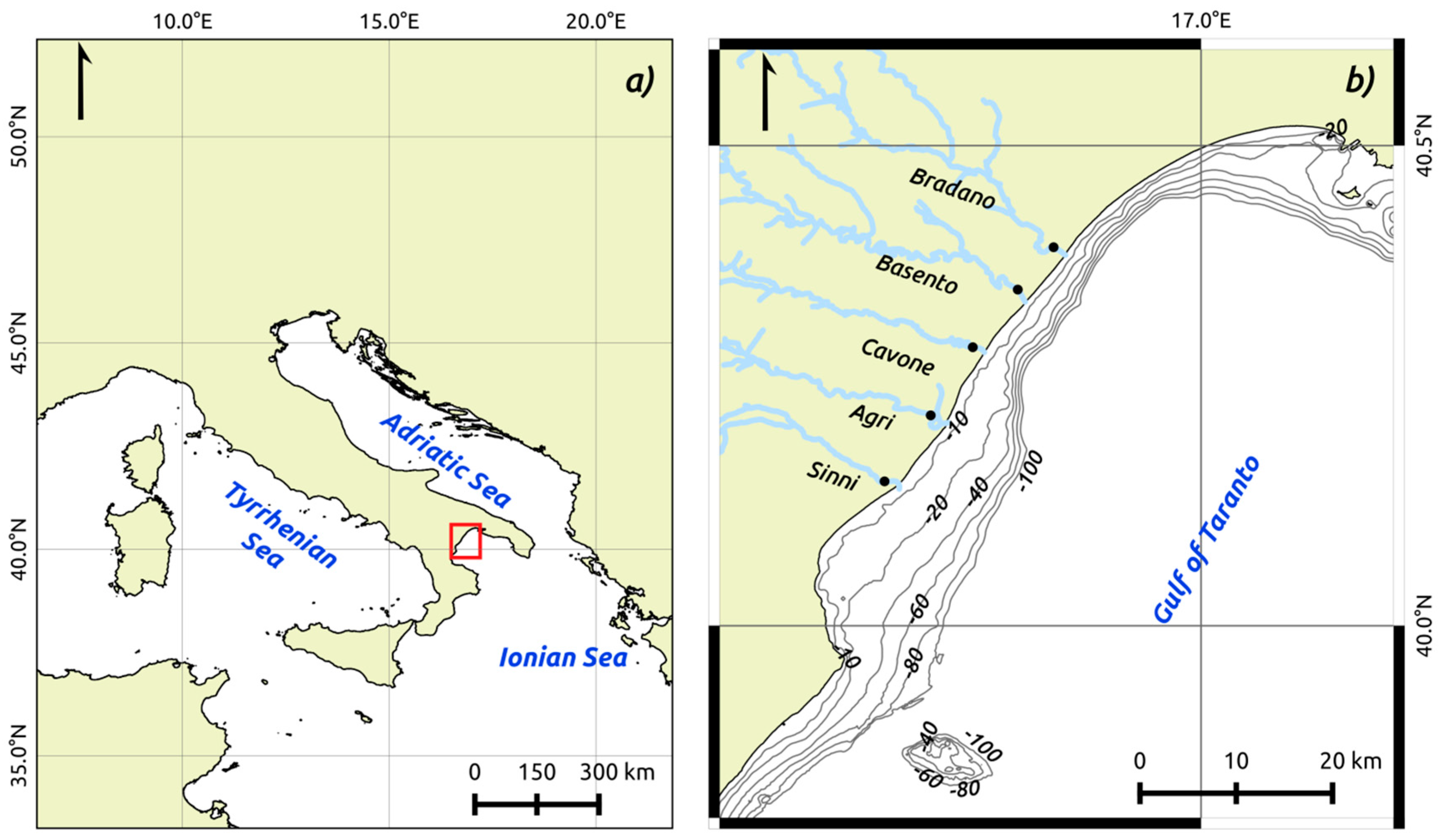
2. Study Area
3. Material and Methods
3.1. Satellite Data Processing for SPM Daily Maps Retrieval
3.2. The RST Approach for Identification of SPM Spatiotemporal Anomalies
4. Results and Discussion
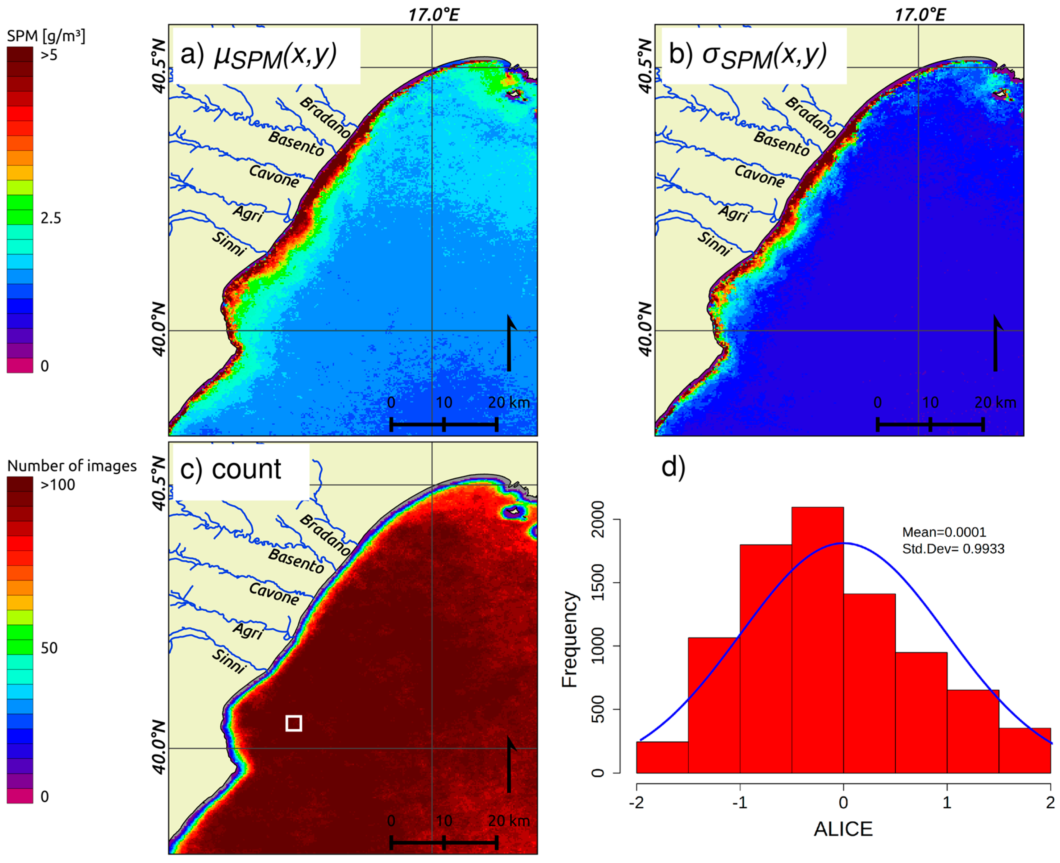
4.1. Interannual Analysis
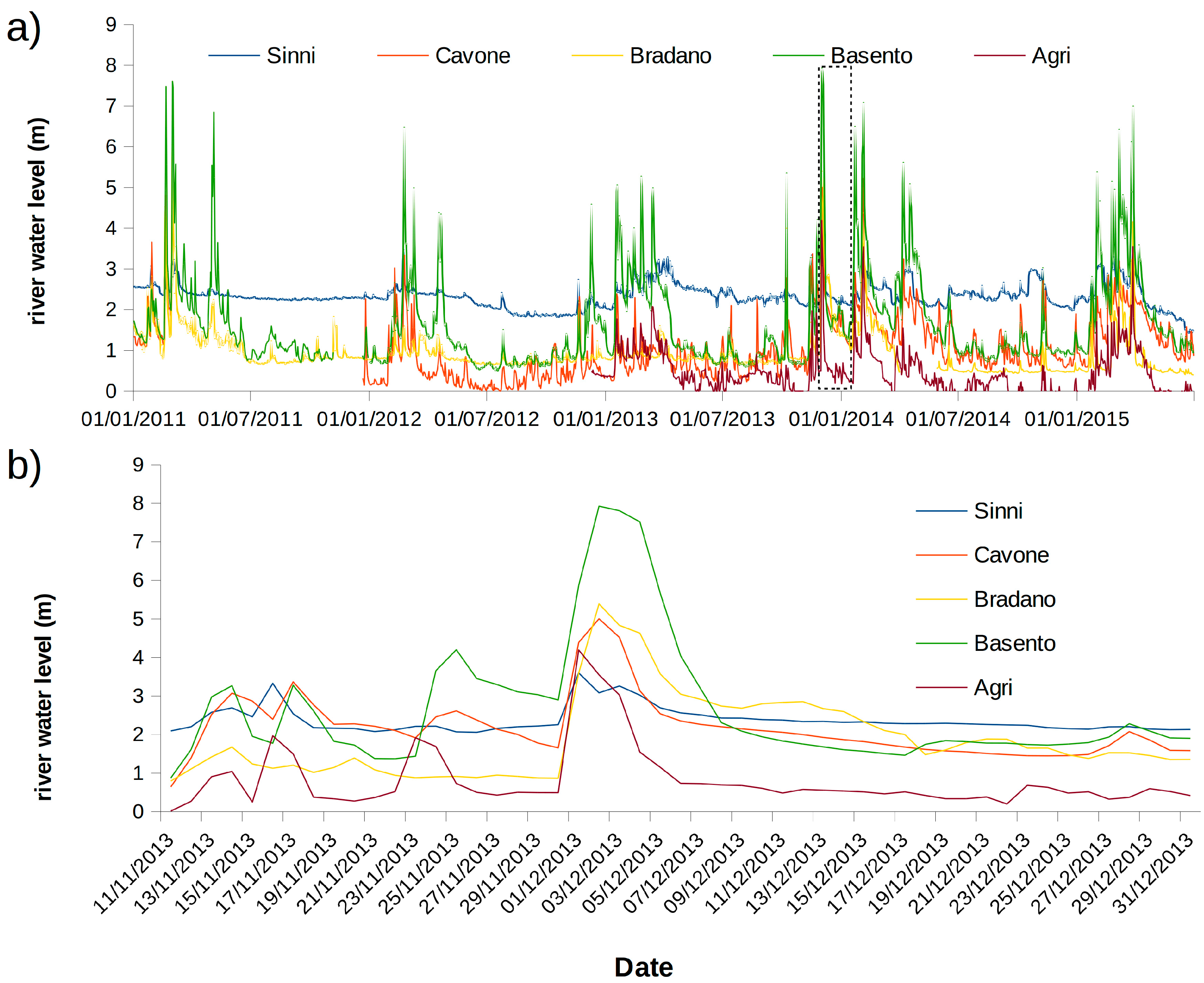
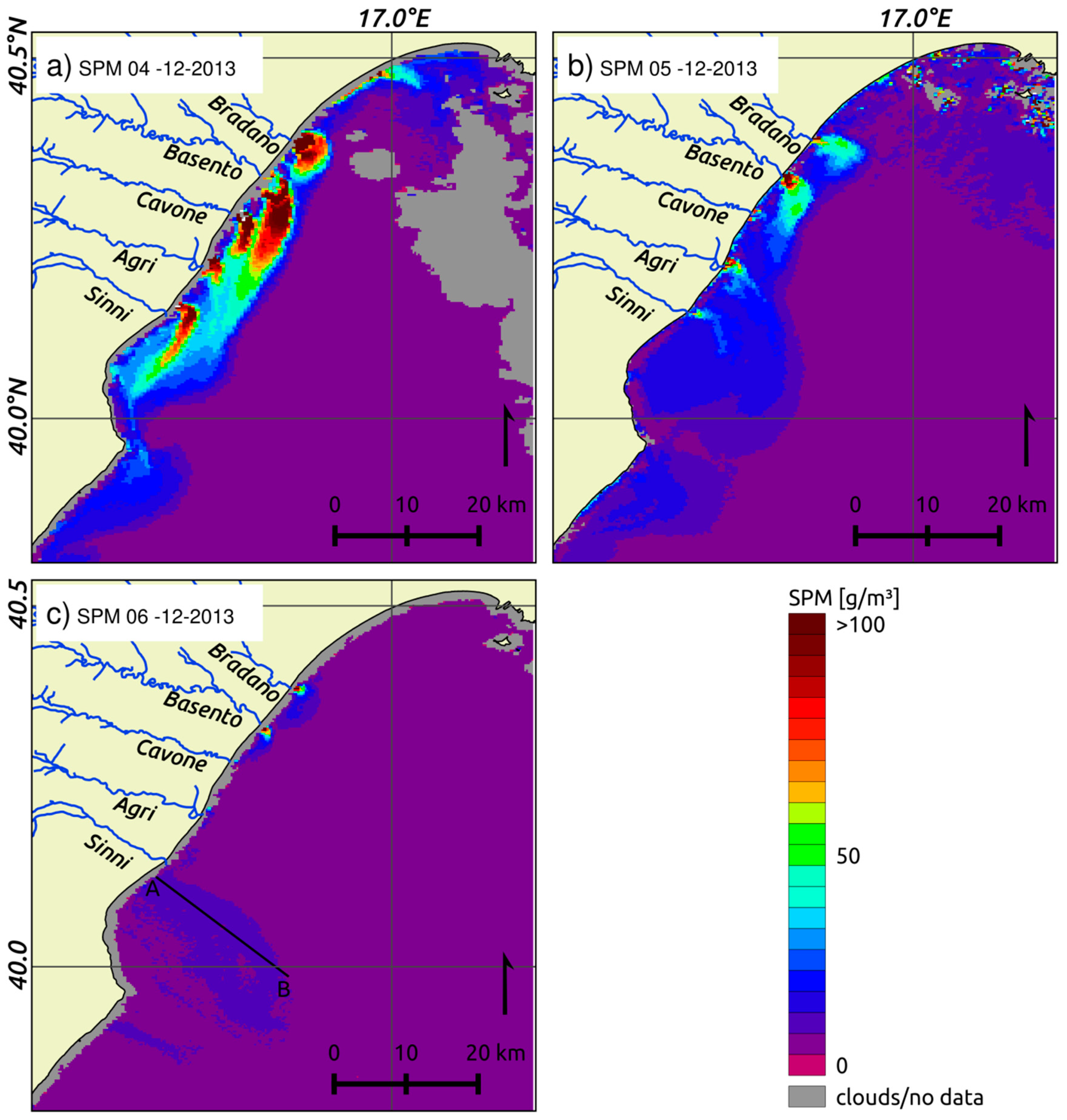
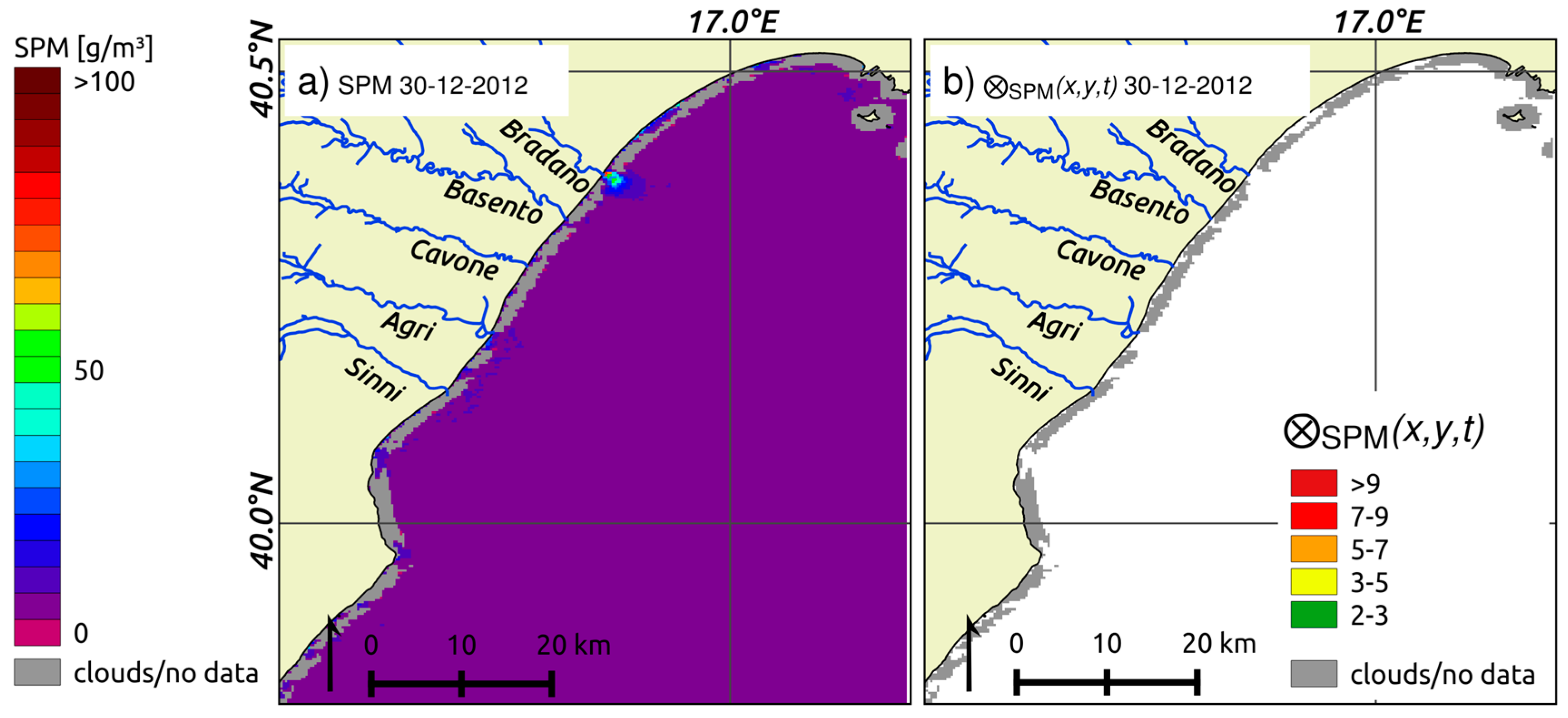
4.2. Daily Analysis for the Event of December 2013
4.3. Evaluation of Wind Effect on SPMc Variation
4.4. Confutation Analysis
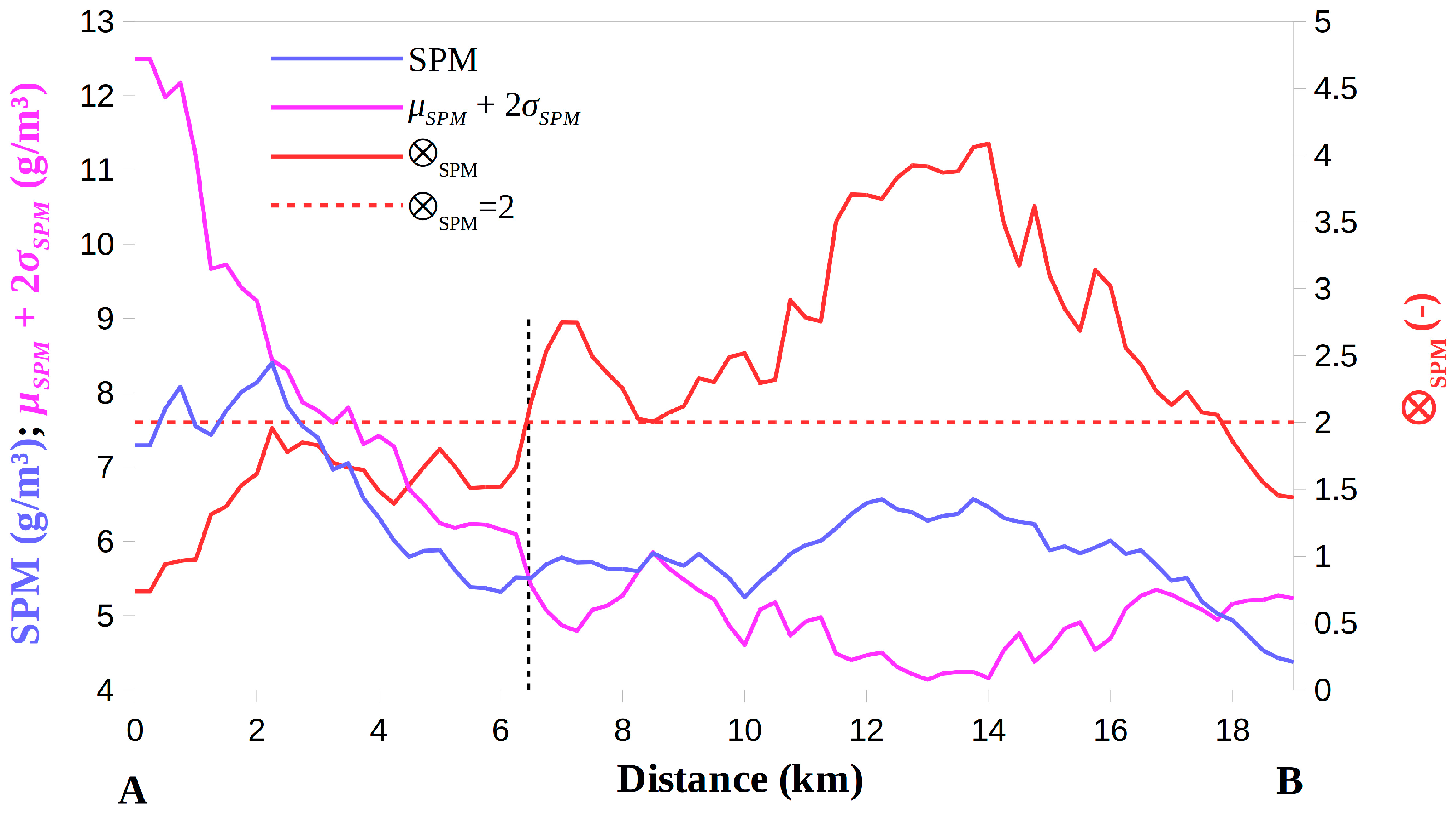
4.5. Identification of the Most Critical Areas in Terms of SPMc Values
5. Conclusions and Prospective
Acknowledgments
Author Contributions
Conflicts of Interest
References
- Miller, R.; McKee, B.A. Using MODIS Terra 250 m imagery to map concentrations of total suspended matter in coastal waters. Remote Sens. Environ. 2004, 93, 259–266. [Google Scholar] [CrossRef]
- Volpe, V.; Silvestri, S.; Marani, M. Remote sensing retrieval of suspended sediment concentration in shallow waters. Remote Sens. Environ. 2011, 115, 44–54. [Google Scholar] [CrossRef]
- European Commission. Directive 60 23 October 2000: Establishing a framework for community action in the field of water policy. Off. J. Eur. Communities 2000, 43, 1–71. [Google Scholar]
- Borja, A.; Galparsoro, I.; Solaun, O.; Muxika, I.; Tello, E.; Uriarte, A.; Valencia, V. The European Water Framework Directive and the DPSIR, a methodological approach to assess the risk of failing to achieve good ecological status. Estuar. Coast. Shelf S. 2005, 66, 84–96. [Google Scholar] [CrossRef]
- Wolanski, E.; Spagnol, S. Pollution by mud of Great Barrier Reef coastal waters. J. Coastal Res. 2000, 16, 1151–1156. [Google Scholar]
- Brown, B.E. Disturbances to reefs in recent times. In Life and Death of Coral Reefs; ITP: Stamford, CT, USA, 1997; pp. 354–379. [Google Scholar]
- Orpin, A.R.; Ridd, P.V.; Thomas, S.; Anthony, K.R.; Marshall, P.; Oliver, J. Natural turbidity variability and weather forecasts in risk management of anthropogenic sediment discharge near sensitive environments. Mar. Poll. Bull. 2004, 49, 602–612. [Google Scholar] [CrossRef]
- Ruhl, C.A.; Schoellhamer, D.H.; Stumpf, R.P.; Lindsay, C.L. Combined use of remote sensing and continuous monitoring to analyse the variability of suspended-sediment concentrations in San Francisco Bay, California. Estuar. Coast. Shelf Sci. 2001, 53, 801–812. [Google Scholar] [CrossRef]
- Maltese, A.; Capodici, F.; Ciraolo, G.; La Loggia, G. Coastal zone water quality: Calibration of a water-turbidity equation for MODIS data. Eur. J. Remote Sens. 2013, 46, 333–347. [Google Scholar] [CrossRef]
- Nechad, B.; Ruddick, K.G.; Park, Y. Calibration and validation of a generic multisensor algorithm for mapping of total suspended matter in turbid waters. Remote Sens. Environ. 2010, 114, 854–866. [Google Scholar] [CrossRef]
- Doxaran, D.; Froidefond, J.; Lavender, S.; Castaing, P. Spectral signature of highly turbid waters Application with SPOT data to quantify suspended particulate matter concentrations. Remote Sens. Environ. 2002, 81, 149–161. [Google Scholar] [CrossRef]
- Hu, C.; Chen, Z.; Clayton, T. Assessment of estuarine water-quality indicators using MODIS medium-resolution bands: Initial results from Tampa Bay, FL, USA. Remote Sens. Environ. 2004, 93, 423–441. [Google Scholar] [CrossRef]
- Min, J.; Ryu, J.; Lee, S. Monitoring of suspended sediment variation using Landsat and MODIS in the Saemangeum coastal area of Korea. Mar. Pollut. Bull. 2012, 64, 382–390. [Google Scholar] [CrossRef]
- Ody, A.; Doxaran, D.; Vanhellemont, Q.; Nechad, B.; Novoa, S.; Many, G.; Bourrin, F.; Verney, R.; Pairaud, I.; Gentili, B. Potential of high spatial and temporal ocean color satellite data to study the dynamics of suspended particles in a micro-tidal river plume. Remote Sens. 2016, 8, 245. [Google Scholar] [CrossRef] [Green Version]
- Dorji, P.; Fearns, P.; Broomhall, M. A semi-analytic model for estimating total suspended sediment concentration in turbid coastal waters of northern Western Australia using MODIS-Aqua 250 m data. Remote Sens. 2016, 8, 556. [Google Scholar] [CrossRef]
- Doxaran, D.; Froidefond, J.; Castaing, P.; Babin, M. Dynamics of the turbidity maximum zone in a macrotidal estuary (the Gironde, France): Observations from field and MODIS satellite data. Estuar. Coast. Shelf Sci. 2009, 81, 321–332. [Google Scholar] [CrossRef]
- Chen, S.; Huang, W.; Chen, W.; Wang, H. Remote sensing analysis of rainstorm effects on sediment concentrations in Apalachicola Bay, USA. Ecol. Inform. 2011, 6, 147–155. [Google Scholar] [CrossRef]
- Wang, J.J.; Lu, X. Estimation of suspended sediment concentrations using Terra MODIS: An example from the Lower Yangtze River, China. Sci. Total Environ. 2010, 408, 1131–1138. [Google Scholar] [CrossRef]
- Kaba, E.; Philpot, W.; Steenhuis, T. Evaluating suitability of MODIS-Terra images for reproducing historic sediment concentrations in water bodies: Lake Tana, Ethiopia. Int. J. Appl. Earth Obs. Geoinf. 2014, 26, 286–297. [Google Scholar] [CrossRef]
- Siswanto, E.; Tang, J.; Yamaguchi, H.; Yuhwan, A.; Ishizaka, J.; Yoo, S.; Sangwoo, K.; Kiyomoto, Y.; Yamada, K.; Chiang, C.; Kawamura, H. Empirical ocean-color algorithms to retrieve chlorophyll-a, total suspended matter, and colored dissolved organic matter absorption coefficient in the Yellow and East China Seas. J. Ocean ogr. 2011, 67, 627–650. [Google Scholar] [CrossRef]
- Han, B.; Loisel, H.; Vantrepotte, V.; Mériaux, X.; Bryère, P.; Ouillon, S.; Dessailly, D.; Xing, Q.; Zhu, J. Development of a semi-analytical algorithm for the retrieval of suspended particulate matter from remote sensing over clear to very turbid waters. Remote Sens. 2016, 8, 211. [Google Scholar] [CrossRef]
- Stumpf, R.P.; Arnone, R.A.; Gould, R.W.; Martinolich, P.M.; Ransibrahmanakhul, V. A partially coupled ocean-atmosphere model for retrieval of water-leaving radiance from SeaWiFS in coastal waters. In SeaWiFS Postlaunch Technical Report Series; Hooker, S.B., Firestone, E.R., Eds.; NASA Goddard Space Flight Center: Greenbelt, MD, USA, 2003; Volume 22, pp. 51–59. [Google Scholar]
- Ruddick, K.; Ovidio, F.; Rijkeboer, M. Atmospheric correction of SeaWiFS imagery for turbid coastal and inland waters. Appl. Opt. 2000, 39, 897–912. [Google Scholar] [CrossRef]
- Wang, M.; Shi, W. The NIR-SWIR combined atmospheric correction approach for MODIS ocean color data processing. Opt. Express 2007, 15, 15722–15733. [Google Scholar] [CrossRef]
- Tramutoli, V. Robust AVHRR Techniques (RAT) for environmental monitoring: Theory and applications. In Earth Surface Remote Sensing II; Cecchi, G., Zilioli, E., Eds.; International Society for Optics and Photonics: Barcelona, Spain, 1998; Volume 3496, pp. 101–113. [Google Scholar]
- Tramutoli, V. Robust Satellite Techniques (RST) for natural and environmental hazards monitoring and mitigation: Ten years of successful applications. In Proceedings of the 9th International Symposium on Physical Measurements and Signatures in Remote Sensing, IGSNRR, Beijing, China, 17–19 October 2005; pp. 792–795.
- Tramutoli, V. Robust Satellite Techniques (RST) for Natural and Environmental Hazards Monitoring and Mitigation: Theory and Applications. In Proceedings of the Fourth International Workshop on the Analysis of Multitemporal Remote Sensing Images, Louven, Belgium, 18–20 July 2007.
- Autorità di Bacino Della Basilicata. Disponibilità: Le Acque Superficiali. Available online: http://www.adb.basilicata.it/adb/pstralcio/bilancioidrico/cap4.pdf (accessed on 2 August 2016).
- Claps, P.; Fiorentino, M. Rapporto di sintesi sulla valutazione delle piene in Italia–Guida Operativa all’applicazione dei rapporti regionali sulla valutazione delle piene in Italia, Linea 1 Previsione e Prevenzione degli eventi idrologici estremi; CNR–GNDCI: Roma, Italy, 1999. [Google Scholar]
- Autorità di Bacino della Basilicata. Available online: http://www.autoritadibacino.basilicata.it/adb/pStralcio/pericol_alluv.asp (accessed on 2 August 2016).
- Matarrese, R.; Chiaradia, M.T.; Tijani, K.; Morea, A.; Carlucci, R. Chlorophyll a multi-temporal analysis in coastal waters with MODIS data. Ital. J. Remote Sens. 2011, 43, 39–48. [Google Scholar]
- Buccolieri, A.; Buccolieri, G.; Cardellicchio, N.; Dell’Atti, A.; Di Leo, A.; Maci, A. Heavy metals in marine sediments of Taranto Gulf (Ionian Sea, Southern Italy). Mar. Chem. 2006, 99, 227–235. [Google Scholar] [CrossRef]
- D’Addabbo, A.; Refice, A.; Pasquariello, G.; Lovergine, F.P.; Capolongo, D.; Manfreda, S. A bayesian network for flood detection combining SAR imagery and ancillary data. IEEE Trans. Geosci. Remote Sens. 2016, 54, 3612–3625. [Google Scholar]
- Piccarreta, M.; Pasini, A.; Capolongo, D.; Lazzari, M. Changes in daily precipitation extremes in the Mediterranean from 1951 to 2010: The Basilicata region, Southern Italy. Int. J. Climatol. 2013, 33, 3229–3248. [Google Scholar] [CrossRef]
- Istituto superiore per la protezione e la ricerca ambientale (ISPRA). La Rete Mareografica Nazionale. Available online: http://www.mareografico.it/ (accessed on 3 November 2016).
- Booth, J.G.; Miller, R.L.; McKee, B.A.; Leathers, R.A. Wind-induced bottom sediment resuspension in a microtidal coastal environment. Cont. Shelf Res. 2000, 20, 785–806. [Google Scholar] [CrossRef]
- Bailey, S.W.; Franz, B.A.; Werdell, P.J. Estimations of near-infrared water-leaving reflectance for satellite oceancolor data processing. Opt. Express 2010, 18, 7521–7527. [Google Scholar] [CrossRef]
- NASA’s Ocean Color Web. Available online: http://oceancolor.gsfc.nasa.gov/cms/ (accessed on 3 November 2016).
- Knaeps, E.; Raymaekers, D.; Sterckx, S.; Ruddick, K.; Dogliotti, A.I. In-situ evidence of non-zero reflectance in the OLCI 1020 nm band for a turbid estuary. Remote Sens. Environ. 2012, 120, 133–144. [Google Scholar] [CrossRef]
- Ruddick, K.G.; De Cauwer, V.; Park, Y.J.; Moore, G. Seaborne measurements of near infrared water-leaving reflectance: The similarity spectrum for turbid waters. Limnol. Ocean 2006, 51, 1167–1179. [Google Scholar] [CrossRef]
- Doron, M.; Bélanger, S.; Doxaran, D.; Babin, M. Spectral variations in the near-infrared ocean reflectance. Remote. Sens. Environ. 2011, 115, 1617–1631. [Google Scholar] [CrossRef]
- Doxaran, D.; Froidefond, J.M.; Castaing, P. Remote-sensing reflectance of turbid sediment-dominated waters. Reduction of sediment type variations and changing illumination conditions effects by use of reflectance ratios. Appl. Opt. 2003, 42, 2623–2634. [Google Scholar] [CrossRef]
- Ciancia, E.; Lourerio, C.M.; Mendonça, A.; Coviello, I.; Di Polito, C.; Lacava, T.; Pergola, N.; Satriano, V.; Tramutoli, V.; Martins, A. On the potential of a RST-based analysis of the MODIS-derived Chl-a product over Condor seamount and surrounding areas (Azores, NE Atlantic). Ocean Dyn. 2016. [Google Scholar] [CrossRef]
- Koeppen, W.C.; Pilger, E.; Wright, R. Time series analysis of infrared satellite data for detecting thermal anomalies: A hybrid approach. Bull. Volcanol. 2011, 73, 577–593. [Google Scholar] [CrossRef]
- Wang, M.; Shi, W. Cloud masking for ocean color data processing in the coastal regions. IEEE Trans. Geosci. Remote Sens. 2006, 44, 3196–3105. [Google Scholar] [CrossRef]
- Lazzari, M.; Gioia, D.; Piccarreta, M.; Danese, M.; Lanorte, A. Sediment yield and erosion rate estimation in the mountain catchments of the Camastra artificial reservoir (Southern Italy): A comparison between different empirical methods. Catena 2015, 127, 323–339. [Google Scholar] [CrossRef]


| SPM (g/m3) | River Level (m) | Wind at Taranto Station (m/s) | |
|---|---|---|---|
| December 2011 | 1.69 | 1.42 | 4.23 |
| December 2012 | 1.29 | 1.26 | 3.65 |
| December 2013 | 2.75 | 2.13 | 2.58 |
| December 2014 | 1.36 | 0.87 | 2.89 |
| December 2015 | 1.20 | 1.03 | 4.61 |
© 2016 by the authors; licensee MDPI, Basel, Switzerland. This article is an open access article distributed under the terms and conditions of the Creative Commons Attribution (CC-BY) license (http://creativecommons.org/licenses/by/4.0/).
Share and Cite
Di Polito, C.; Ciancia, E.; Coviello, I.; Doxaran, D.; Lacava, T.; Pergola, N.; Satriano, V.; Tramutoli, V. On the Potential of Robust Satellite Techniques Approach for SPM Monitoring in Coastal Waters: Implementation and Application over the Basilicata Ionian Coastal Waters Using MODIS‐Aqua. Remote Sens. 2016, 8, 922. https://doi.org/10.3390/rs8110922
Di Polito C, Ciancia E, Coviello I, Doxaran D, Lacava T, Pergola N, Satriano V, Tramutoli V. On the Potential of Robust Satellite Techniques Approach for SPM Monitoring in Coastal Waters: Implementation and Application over the Basilicata Ionian Coastal Waters Using MODIS‐Aqua. Remote Sensing. 2016; 8(11):922. https://doi.org/10.3390/rs8110922
Chicago/Turabian StyleDi Polito, Carmine, Emanuele Ciancia, Irina Coviello, David Doxaran, Teodosio Lacava, Nicola Pergola, Valeria Satriano, and Valerio Tramutoli. 2016. "On the Potential of Robust Satellite Techniques Approach for SPM Monitoring in Coastal Waters: Implementation and Application over the Basilicata Ionian Coastal Waters Using MODIS‐Aqua" Remote Sensing 8, no. 11: 922. https://doi.org/10.3390/rs8110922