A Spectral-Texture Kernel-Based Classification Method for Hyperspectral Images

Abstract

Classification of hyperspectral images always suffers from high dimensionality and very limited labeled samples. Recently, the spectral-spatial classification has attracted considerable attention and can achieve higher classification accuracy and smoother classification maps. In this paper, a novel spectral-spatial classification method for hyperspectral images by using kernel methods is investigated. For a given hyperspectral image, the principle component analysis (PCA) transform is first performed. Then, the first principle component of the input image is segmented into non-overlapping homogeneous regions by using the entropy rate superpixel (ERS) algorithm. Next, the local spectral histogram model is applied to each homogeneous region to obtain the corresponding texture features. Because this step is performed within each homogenous region, instead of within a fixed-size image window, the obtained local texture features in the image are more accurate, which can effectively benefit the improvement of classification accuracy. In the following step, a contextual spectral-texture kernel is constructed by combining spectral information in the image and the extracted texture information using the linearity property of the kernel methods. Finally, the classification map is achieved by the support vector machines (SVM) classifier using the proposed spectral-texture kernel. Experiments on two benchmark airborne hyperspectral datasets demonstrate that our method can effectively improve classification accuracies, even though only a very limited training sample is available. Specifically, our method can achieve from 8.26% to 15.1% higher in terms of overall accuracy than the traditional SVM classifier. The performance of our method was further compared to several state-of-the-art classification methods of hyperspectral images using objective quantitative measures and a visual qualitative evaluation.

1. Introduction

With the development of hyperspectral imaging technology, hyperspectral images with over a hundred of spectral bands, together with increasing spatial resolution, can be simultaneously acquired. In a hyperspectral image, each band includes rich spatial structure information, while each pixel contains many spectral features across a continuous range of narrow channels, from which arouses many real-world applications of hyperspectral images [1]. Meanwhile, the high dimensionality of hyperspectral images, along with limited labeled samples [2], present challenges to image classification, such as the Hughes phenomenon [3]. To overcome these problems, many pixel-wise classification methods have been proposed by using spectral information of hyperspectral images, including normal classification methods like Bayesian models [4,5], random forests [6], neural networks [7,8], SVMs [9,10,11], kernel methods [12] and semi-supervised learning methods [13].

However, the resultant classification maps by those methods are always corrupted by salt-and-pepper class noise, due to the fact that those pixel-wise classifiers only utilize spectral information without considering spatial dependencies of neighboring pixels in the same class. To further improve classification accuracy and smoothness of classification maps, spectral-spatial classification has attracted considerable attention [2,14]. The two most common approaches are: (1) integrating the spatial contextual and the spectral information into the pixel-wise classifiers; (2) extracting the spectral and the spatial information separately and then combining the two results to obtain a final classification map.

The approaches in the first category include using grey level co-occurrence matrix (GLCM) [15,16], extended morphological profiles (EMPs) [17], extended morphological attribute profiles (EAPs) [18], Gabor filtering [19,20] and Markov random fields (MRF) [21,22] to obtain spectral-spatial features. Another approach to use the spatial information is to utilize spectral-spatial kernels, including composite [23], morphological [24] and graph [25] kernels, to improve the performance of the SVM classifier.

The second category for performing spectral-spatial classification was achieved by different segmentation techniques of watershed [26], mean shift [27,28], hierarchical segmentation [29,30], superpixel segmentation [31], extraction and classification of homogeneous objects (ECHO) [32], minimum spanning forest [33] and graph cut [34,35], etc. After the segmentation process, hyperspectral images are partitioned into many small regions and all pixels in each region of the segmentation map have similar spatial features. To label these regions, two commonly used techniques can be adopted. The first one is to use a supervised classifier to directly classify those regions and pixels in each region are assigned with the same label [24]. While the second one is to combine a pixel-wise classification map and a region-based segmentation map to produce a final spectral-spatial classification map by using majority voting [26,33] or class labels of automatically selected markers [29]. If a maximum vote decision rule is used, the class label of each region is determined by the most frequent class in the same region according to the pixel-wise classification map; while if representative spectra in hyperspectral images are automatically extracted, the marker-based segmentation algorithm can be performed to obtain a segmentation map, in which class labels of those homogeneous regions are determined by that of markers obtained by a pixel-wise classifier.

With the development of hyperspectral image sensors, spatial resolution of hyperspectral images has greatly increased as well as spectral resolution and richer texture information can be acquired to characterize ground objects in hyperspectral images. It is widely known that a visual texture is very difficult to characterize [36]. In general, morphological operations are often used to represent texture information, but those operations cannot effectively characterize complex texture features due to limited forms of operations. It is well known that texture descriptors are powerful features for texture synthesis and discrimination and can be obtained by convolving an image with a bank of filters tuned to different orientations and spatial frequencies. To obtain satisfactory classification results, we expect to integrate texture information with spectral information in the classification process, which enables improved performance of discriminating land covers.

With this motivation, we present a novel spectral-spatial classification method for hyperspectral images by using kernel methods, which consists of five main steps. For a given hyperspectral image, the PCA transform is first performed. Second, the first principle component of the input hyperspectral image is segmented into nonoverlapping homogeneous regions by using the ERS algorithm [37]. Third, the local spectral histogram model is applied to each homogeneous region to obtain the corresponding texture features. Because this step is performed within each homogenous region obtained by the segmentation process, instead of within a fixed-size image window proposed in the original work of [38,39], the obtained local texture features in the image are more accurate, which can effectively benefit the improvement of classification accuracy. In the next step, a contextual spectral-texture kernel is constructed by combining spectral information in the image and the extracted texture information using the linearity property of the kernel methods [23,40]. Finally, the classification map is achieved by the SVM-based classifier using the proposed spectral-texture kernel. Our method is superior to the state-of-the-art spectral-spatial classification methods in terms of classification accuracy, because the segmentation-based texture representation is more efficient way to locally characterize spatial structure features in the image.

The remainder of this paper is organized as follows. Section 2 reviews the techniques of the ERS segmentation and the spectral histogram model. Section 3 presents the proposed spectral-texture kernel-based classification method for hyperspectral images. Section 4 reports the experimental results, Section 5 discusses some issues of the proposed method and the last section states our concluding remarks.

2. Related Techniques

2.1. Entropy Rate Superpixel Segmentation

Liu et al. [37] formulated the superpixel segmentation problem as an optimization problem on a graph and presented a corresponding objective function on the graph topology by integrating the entropy rate and the balancing function. We map an image u to an undirected graph $\mathrm{G}=(\mathrm{V},\mathrm{E})$ with the set of vertices V corresponding to the pixels in the image and the set of edges E that occur between any two pixels u_i and u_j within a small distance of each other. The aim of the ERS segmentation is to select a subset of edges $\mathrm{A}\subseteq \mathrm{E}$ and the obtained graph $\mathrm{G}=(\mathrm{V},\mathrm{A})$ contains K connected subgraphs. The clustering process can be formulated as the following objective function:

$$\begin{gathered} \underset{\mathrm{A}}{\max }H\left(\mathrm{A}\right)+\lambda B\left(\mathrm{A}\right) \\ \text{subject to} \mathrm{A}\subseteq \mathrm{E} \text{and} N_{\mathrm{A}}\ge K \end{gathered}$$

(1)

where λ (λ > 0) is the weight of the balancing term. H(A) denotes the entropy rate of the random walk on a graph and is used as a measure to obtain compact and homogeneous clusters. This term can be defined as a set of function as follows:

$$H\left(\mathrm{A}\right)=-{\displaystyle \sum _i{\alpha }_i}{\displaystyle \sum _j{p}_{i,j}\left(\mathrm{A}\right)\log \left(p_{i,j}\left(\mathrm{A}\right)\right)}$$

(2)

where ${\alpha }_i=w_i/w_T$, $w_i$ is the sum of the weights of the edges connected with the ith vertex and $w_T={\displaystyle \sum _{i=1}^{\left|\mathrm{V}\right|}{w}_i}$ is the normalization constant, where $\left|\mathrm{V}\right|$ is the total number of vertices in the graph. $p_{i,j}$ is the transition probability. Let the graph partitioning for the edge set A be $T_{\mathrm{A}}=\left\{T_1,T_2,...,T_{N_{\mathrm{A}}}\right\}$, Z_A be the distribution of the cluster membership and N_A be the total number of connected components with respect to A in the graph, the distribution of Z_A is then defined as follows:

$$p{Z}_{\mathrm{A}}\left(i\right)=\frac{\left|T_i\right|}{\left|\mathrm{V}\right|},i=\left\{1,2,...,N_{\mathrm{A}}\right\}$$

(3)

and the balancing term, which is used to favor clusters with similar sizes, is given by

$$B\left(\mathrm{A}\right)=-{\displaystyle \sum _{i}p{Z}_{\mathrm{A}}\left(i\right)\log \left(p{Z}_{\mathrm{A}}\left(i\right)\right)}-N_{\mathrm{A}}$$

(4)

We refer the reader to Liu et al. [37] for details on the ERS segmentation algorithm.

2.2. The Spectral Histogram Model

Given an input image window W and a bank of filters $\left\{F^{\left(\alpha \right)},\alpha =1,2,...,M\right\}$, where M is the total number of different filters, we can obtain a set of images $\left\{{\mathbf{W}}^{\left(1\right)},{\mathbf{W}}^{\left(2\right)},...,{\mathbf{W}}^{\left(M\right)}\right\}$ by linear convolution, namely, ${\mathbf{W}}^{\left(\alpha \right)}\left(n\right)=F^{\left(\alpha \right)}\ast \mathbf{W}\left(n\right)={\displaystyle \sum _m{F}^{\left(\alpha \right)}\left(m\right)\mathbf{W}\left(n-m\right)}$, where m and n represent pixel locations. The histogram of ${\mathbf{W}}^{\left(\alpha \right)}$ can be given as follows [38,39,41]:

$$H_{\mathbf{W}}^{(\alpha )}\left(t_1,t_2\right)={\displaystyle \sum _{n\in \mathbf{W}}{\displaystyle {\int }_{t_1}^{t_2}\delta }\left(t-{\mathbf{W}}^{(\alpha )}\left(n\right)\right)dt}$$

(5)

where $t_1$ and $t_2$ specify the range of the bin. Therefore, the spectral histogram corresponding to the specific bank of filters can be defined as follows [38,39,41]:

$$H_{\mathbf{W}}=\frac{1}{\left|\mathbf{W}\right|}(H_{\mathbf{W}}^{(1)},H_{\mathbf{W}}^{(2)},\dots ,H_{\mathbf{W}}^{(M)})$$

(6)

where $\left|\mathbf{W}\right|$ is the cardinality of W. According to Equation (6), the spectral histogram of an image is essentially a vector consisting of marginal distributions of responses of different filters. The spectral histogram model is an effective tool for capturing texture appearance, because it is capable of representing both local and global patterns by adopting proper filters [41], such as the Dirac delta function, Laplacian of Gaussian (LoG) filters and Gabor filters, etc. Those classical filters are briefly introduced as follows:

(i)

Ideally, optical remote sensing systems should have the same property of a Dirac delta function, which records the intensity value at a pixel location.

$$\delta \left(x\right)=\{\begin{array}{cc}0& t\ne 0\\ \infty & t=0\end{array}$$

(7)

and which is also constrained to satisfy the identity

$${\displaystyle {\int }_{-\infty }^{\infty }\delta \left(x\right)}dx=1$$

(8)

(ii)

Laplacian filters are derivative filters for detecting areas of edges in images. Since derivative filters are very sensitive to noise, it is common to perform Gaussian smoothing on the image before applying the Laplacian. This two-step process is named as the LoG operation:

$$\mathrm{LoG}\left(x,y|{\sigma }_{\mathrm{LoG}}\right)=\frac{1}{\pi {\sigma }_{\mathrm{LoG}}^4}\left(\frac{x^2+y^2}{2{\sigma }_{\mathrm{LoG}}^2}-1\right){\mathrm{e}}^{-(x^2+y^2)/2{\sigma }_{\mathrm{LoG}}^2}$$

(9)

where ${\sigma }_{\mathrm{LoG}}$ is the standard deviation of the Gaussian function used in the LoG filters.

(iii)

Gabor filters are generally used for edge detection and texture extraction. and are special classes of bandpass filters, i.e., they allow a certain ‘band’ of frequencies and reject the others. The Gabor filter is defined as follows:

$$\mathrm{Gabor}\left(x,y|{\sigma }_{\mathrm{Gabor}},\theta \right)=e^{-\left[{\left(x\cos \theta +y\sin \theta \right)}^2+{\left(-x\sin \theta +y\cos \theta \right)}^2\right]/2{\sigma }_{\mathrm{Gabor}}^2}\cos \left[\frac{2\pi }{\beta }\left(x\cos \theta +y\sin \theta \right)\right]$$

(10)

where ${\sigma }_{\mathrm{Gabor}}$ is the standard deviation of the Gaussian function used in the Gabor filter, θ specifies the orientation of the normal to the parallel stripes of the Gabor function and the ratio ${\sigma }_{\mathrm{Gabor}}/\beta$ is set to 0.5.

3. Spectral-Texture Kernel-Based Classification Method

In this work, a spectral-spatial classification method for hyperspectral images by using kernel methods is proposed. A flow-chart of our classification approach is summarized in Figure 1. First, the first principle component of an input hyperspectral image is partitioned into nonoverlapping homogeneous regions by using the ERS segmentation algorithm [37]. Second, a local spectral histogram representation technique is applied to each homogeneous region to obtain texture descriptors, which consist of histograms of filter responses in the corresponding region. Third, a contextual spectral-texture kernel is constructed by combining spectral information and the extracted texture information, which are integrated using the linearity property of the kernel methods. Finally, the final classification map is achieved by the SVM-based classifier using the proposed spectral-texture kernel.

3.1. Structure Areas Generation

In this work, structure areas are obtained by using the ERS segmentation algorithm. To mitigate computational burden, the linear PCA transform method is performed on the input hyperspectral image, with the first principle component (PC 1) of the hyperspectral image serving as the base image. It is known that the first principle component, corresponding to the highest eigenvalue, contains the most abundant information of the data. The required texture features are extracted based on this component as well.

3.2. Texture Features Extraction

Once the structure areas are obtained, we extract texture features from the base image, namely, the first principle component of the input image. The task of this step is to select the most informative features for classification and we can adopt the existing feature extractors with commonly used methods, such as GLCM, wavelet, etc. Yuan et al. [39] applied the local spectral histogram model to segment high resolution remote sensing images and demonstrated promising experimental results. Following this work, three kinds of filters are used in our method, i.e., the intensity, LoG and Gabor filters, because those filters are very effective and can be easily implemented. Furthermore, different combinations of those filters can achieve promising results, as discussed in Section 5.1. As described in the original work of [38,39,41], the local spectral histogram is computed within a fixed-size image window. However, the extraction of texture descriptors is performed by our method within each structure area in the ERS segmentation map. Specifically, texture features of the base image are extracted by using LoG filters, Gabor filters and the intensity filter. In addition, then, the texture features in each structure area are used as input variables in the Model (6) to obtain the spectral histogram for this area. Therefore, each pixel in the same structure area has an identical spectral histogram. As a consequence, each pixel in the image has both spectral and texture information, i.e., the spectral information is its vector value and the texture information is represented by its texture features obtained by the spectral histogram of a specific structure area that this pixel belongs to.

3.3. Spectral-Texture Support Vector Machines

Based on the explanations in Section 3.2, we can produce a new image, in which each pixel is a stacked vector including both spectral and texture information, and perform spectral-spatial classification by classifying this image using a pixel-wise classifier. However, the optimal methods for integrating these two types of information (spectral and spatial) in the classification process is still an open problem. In this subsection, an effective technique of combining these two types of information by using a contextual spectral-texture kernel-based SVM classifier is introduced.

The classical SVM classifier is well suitable for classifying hyperspectral images when only a limited number of training samples is available. Details on SVM can be referred to [9,42]. When applying SVM, the Gaussian radial basis function (RBF) kernel is widely used as follows:

$$k_{\sigma }\left(\mathbf{x},\mathbf{y}\right)=\exp \left(-\frac{{\Vert \mathbf{x}-\mathbf{y}\Vert }^2}{2{\sigma }^2}\right)$$

(11)

where $\Vert \cdot \Vert$ is the norm based on the Euclidean distance, σ is the standard deviation of the Gaussian function used in the RBF kernel, x and y represent two spectral feature vectors in some input space, respectively. As mentioned in Section 1, spatial dependencies between adjacent pixels are not taken into account in the pixel-wise SVM classifier.

Let ${\mathbf{x}}^{spect}$ and ${\mathbf{y}}^{spect}$ be two spectral feature vectors in some input space, respectively, ${\mathbf{x}}^{text}$ and ${\mathbf{y}}^{text}$ be two texture vector features obtained from Equation (6), respectively, and ${\sigma }_{\mathrm{STK}}$ be the standard deviation of the Gaussian function in the proposed kernel. As stated in [23,40] on rules for kernel construction, if both $k_1$ and $k_2$ are kernels, then $\mu k_1+\left(1-\mu \right)k_2$ is a kernel as well with $0<\mu <1$. According to this property, we can present a novel composite kernel by integrating both spectral and texture information as follows:

$$k_{{\sigma }_{\mathrm{STK}}}^{spect-text}\left(\mathbf{x},\mathbf{y}\right)=\left(1-\mu \right)k_{{\sigma }_{\mathrm{STK}}}^{spect}\left({\mathbf{x}}^{spect},{\mathbf{y}}^{spect}\right)+\mu k_{{\sigma }_{\mathrm{STK}}}^{text}\left({\mathbf{x}}^{text},{\mathbf{y}}^{text}\right)$$

(12)

where μ ($0<\mu <1$) is the weight to balance spatial and texture information in the proposed kernel $k_{{\sigma }_{\mathrm{STK}}}^{spect-text}$. If $\mu =0$, $k_{{\sigma }_{\mathrm{STK}}}^{spect-text}$ changes to the spectral kernel $k_{{\sigma }_{\mathrm{STK}}}^{spect}$ which can be formulated as the RBF kernel Equation (11). As the increase of μ, the relative proportion of texture information becomes higher in the proposed kernel. When μ increases to 1, a kernel with only texture information is obtained. In Equation (12), $k_{{\sigma }_{\mathrm{STK}}}^{text}$ is a texture kernel defined as follows:

$$k_{{\sigma }_{\mathrm{STK}}}^{text}\left({\mathbf{x}}^{text},{\mathbf{y}}^{text}\right)=\exp \left(-\frac{{\Vert {\mathbf{x}}^{text}-{\mathbf{y}}^{text}\Vert }^2}{2{\sigma }_{\mathrm{STK}}^2}\right)$$

(13)

It is reasonable to use the same standard deviation of the Gaussian function in both the spectral and texture kernels due to the fact that the texture features are extracted using the spectral histogram model from the first principle component of the input image, which is the composite spectral information of all bands. Finally, the spectral-texture kernel (STK) based classification algorithm (Algorithm 1) of hyperspectral images is briefly described as follows:

Algorithm 1. STK Based Classification Algorithm

Input: An original hyperspectral image u, the available training samples Step 1: Initialize the number of segments nb_seg; Step 2: Obtain the first principle component of u using the PCA transform; Step 3: Perform the ERS segmentation according to Equation (1) on the first principle component map obtained from Step 2; Step 4: Convolve the first component map separately with the Dirac delta function, the LoG filter and the Gabor filter according to Equations (7)–(10); Step 5: Compute for each structure area in segmentation map obtained from Step 3 the corresponding spectral histogram according to Equations (5)–(6) using textures features extracted from Step 4; Step 6: Apply the supervised multiclass One vs. All SVM classifier with the proposed spectral-texture kernel according to Equation (12) to classify u by adopting the randomly selected training samples; Step 7: Obtain the resultant classification map.

4. Results

4.1. Evaluation Measures

In this section, the proposed STK method was used for classifying three benchmark airborne hyperspectral datasets. To evaluate the effectiveness of our method, seven competitive methods including several state-of-the-art spectral-spatial classifiers were chosen for comparison as follows:

(1)

The pixel-wise SVM classifier with a Gaussian RBF kernel. The parameters of the classifier were determined for each dataset in the following experiments.

(2)

The spectral-spatial kernel-based classifier (SSK) [43] using a morphological area filter with a size of 30, a vector median filter and a contextual spectral-spatial SVM classifier with a Gaussian RBF kernel.

(3)

The spectral-spatial extended EMP classifier [17]. The EMP was constructed based on the first three principal components of a hyperspectral image, a flat disk-shaped structuring element with radius from 1 to 17 with a step of 2, and the number of openings/closings is 8 for each principle component.

(4)

An edge-preserving filter based spectral-spatial classifier [44]. A joint bilateral filter was applied to a binary image for edge preservation and the first principal component of a hyperspectral image was employed as a guidance image. In this work, this classifier was named as EPF-B and its parameters were set as ${\sigma }_s=1$ and ${\sigma }_r=0.1$.

(5)

The Multinomial logistic regression (MLR) algorithm [45] which is learnt using the logistic regression via variable splitting and augmented Lagrangian (LORSAL) algorithm [46]. In this work, this classifier was named as MLR-LORSAL.

(6)

The spectral-spatial classifier using loopy belief propagation and active learning (LBP-AL) [45].

(7)

The logistic regression via splitting and augmented Lagrangian-multilevel logistic classifier with active learning (LORSAL-AL-MLL) [47].

In the following experiments, our method was implemented by the LIBSVM software [48,49] with the proposed spectral-texture kernel, in which five filters were used, i.e., two LoG filters with ${\sigma }_{\mathrm{LoG}}=0.5$ and ${\sigma }_{\mathrm{LoG}}=1$, two Gabor filters with the $\theta =0^{°}$, $\theta ={90}^{°}$ and ${\sigma }_{\mathrm{Gabor}}=1.5$, and the intensity filter. Meanwhile, the penalty term C and ${\sigma }_{\mathrm{STK}}$ in the spectral-texture kernel were set to 200 and 0.5, respectively, while the weight μ was determined for each dataset. Each original dataset including spectral and texture feature maps was scaled between [0,1] using a channel-wise stretching method.

In our experiments, the source codes of the MLR-LORSAL, LBP-AL and LORSAR-AL-MLL methods are available on Li’s homepage (http://www.lx.it.pt/~jun). The parameters of these methods were set to the default values as in [45,46,47].

To evaluate these methods, several assessment measures were used as follows:

(1)

Objective measures including three widely used global accuracy (GA) measures of the overall accuracy (OA), the average accuracy (AA) and the kappa coefficient (κ), and the class-specific accuracy (CA), which can be computed from a confusion matrix based on the ground truth data.

(2)

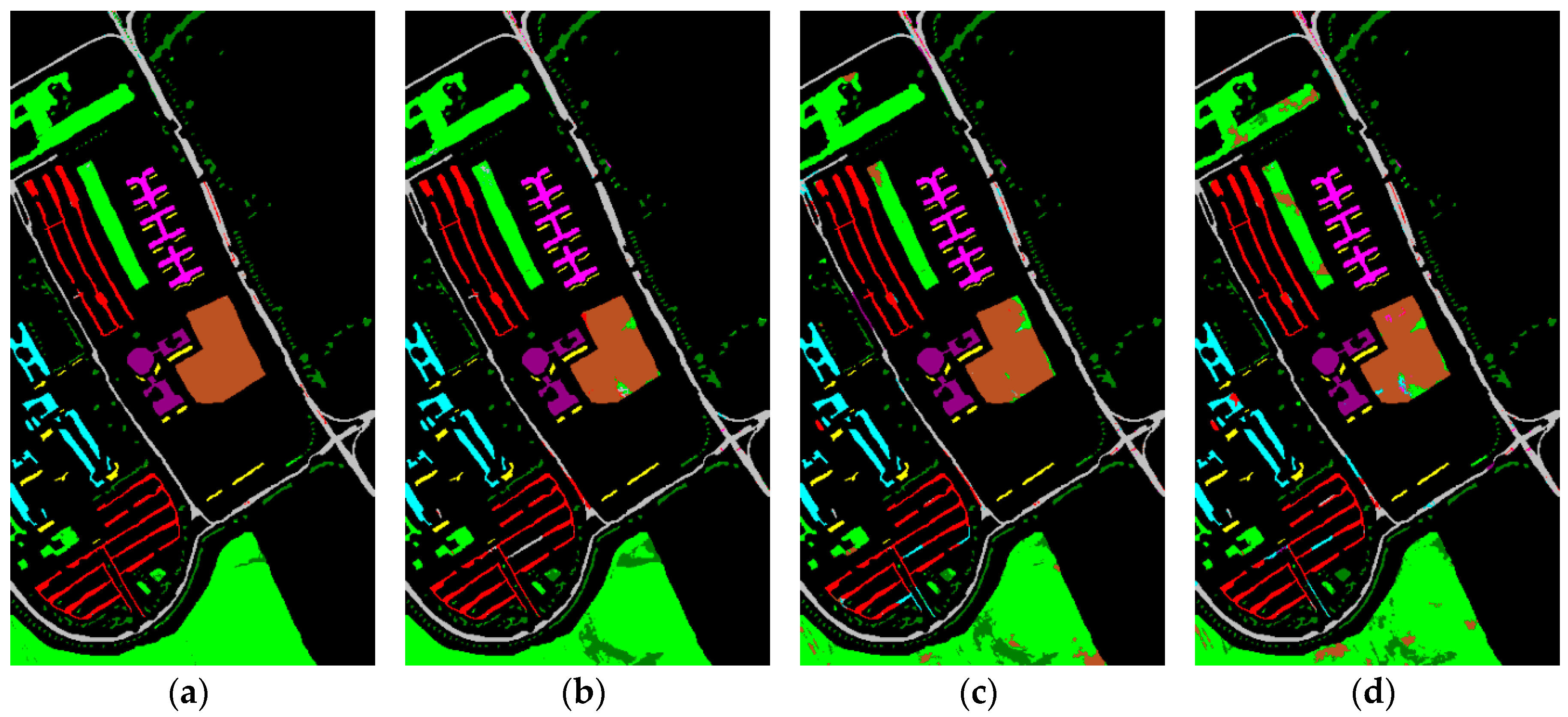
Subjective measure: visual comparison of classification maps.

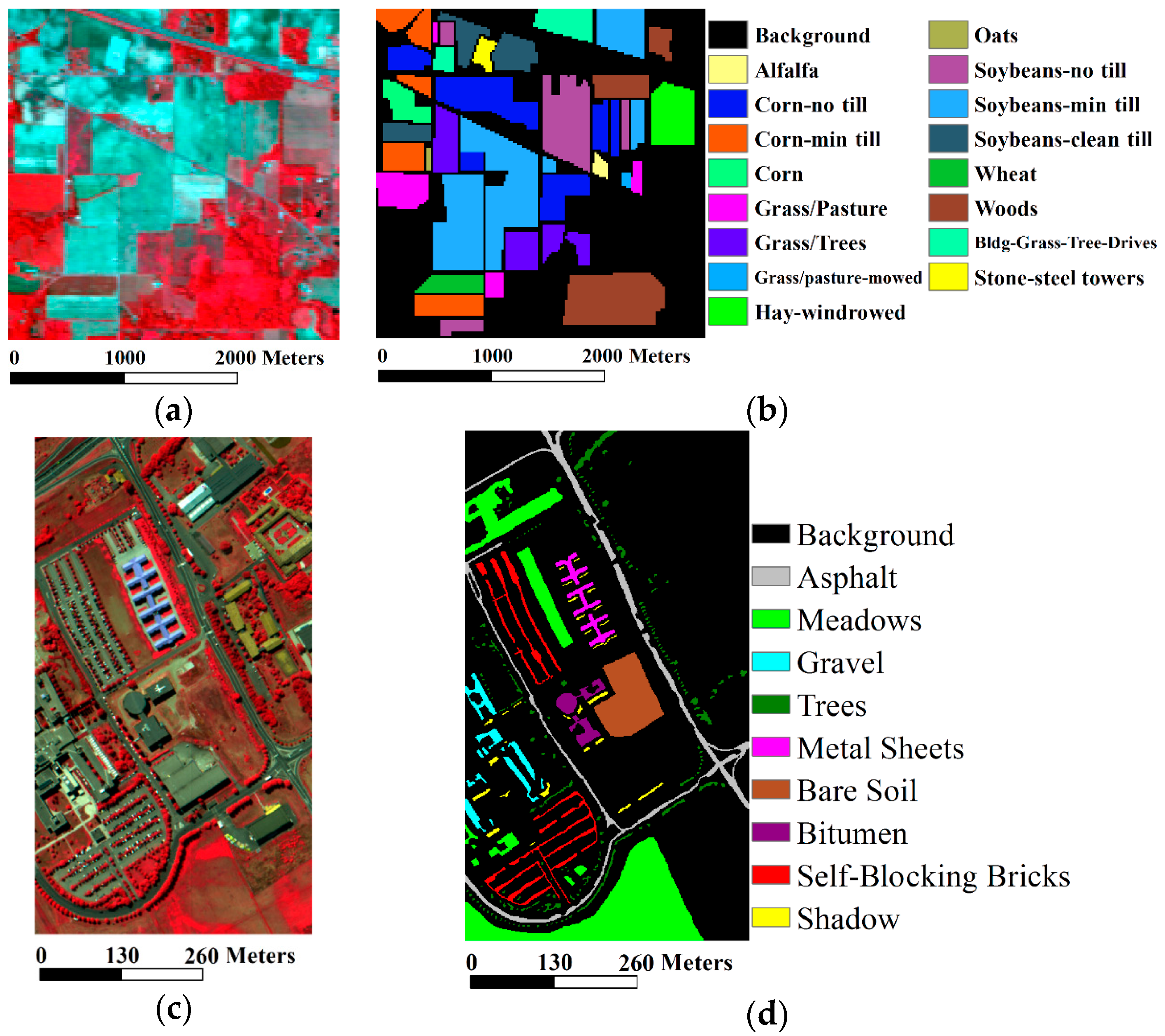
4.2. Data Descriptions

The first image was captured by Airborne Visible Infrared Imaging Spectrometer (AVIRIS) over the agricultural Indian Pines test site of northwestern Indiana on 12 June 1992 taken on a NASA ER2 flight at high altitude with a ground pixel size of 17 m resolution. This image is of size 145 × 145 × 220 of reflectance data with about two-thirds agriculture and one-third forest or other natural perennial vegetation. According to Tadjudin and Landgrebe’s work [50] and the later work of Duarte et al. [51], we reduced the number of bands to 185 by removing bands 1–3, 58, 77, 103–110, 148–166 and 218–220 covering the region of water absorption or too noisy. The reference data available covered 49% of the image and it is divided among sixteen classes of interest ranging in size from 20 pixels to 2468 pixels. The hyperspectral data and the corresponding reference data are available from the work of [52]. A false color composite of the Indian Pines image, with bands of 47 (860.28 nm), 23 (646.72 nm) and 13 (547.6 nm), and the corresponding reference data are shown in Figure 2a,b.

The second image was recorded by the Reflective Optics System Imaging Spectrometer (ROSIS-03) optical sensor. The flight over the city of Pavia, Italy, was operated by the Deutschen Zentrum fur Luft-und Raumfahrt (DLR, the German Aerospace Agency) in the framework of the HySens project, and managed and sponsored by the European Union. The ROSIS-03 sensor can produce an image with a spatial resolution of 1.3 m per pixel and 115 bands ranging from 430 to 860 nm. This University of Pavia image is 610 × 340 pixels and 103 spectral bands with the heavy noisy bands (12) discarded. The image was atmospherically corrected but not geometrically corrected. Nine classes of interest were considered for classification, i.e., trees, asphalt, bitumen, gravel, metal sheets, shadow, self-blocking bricks, meadows, and bare soil. According to the work of [53], the hyperspectral data and the corresponding reference data are available from the FTP website (http://tlclab.unipv.it/downloads/1/20091123/HYSENS.zip) provided by Paolo Gamba. A RGB color composite map obtained from bands 103 (838 nm), 56 (650 nm) and 31 (550 nm) of the University of Pavia image and the corresponding reference data are shown in Figure 2c,d.

To establish the performance of the supervised support vector classifier, we chose a number of training and test samples for each hyperspectral dataset based on the reference data in Figure 2. For the Indian Pines image, a fixed 10 percent of the known reference data were randomly selected for each class as the training set (if the selected number of training samples was less than ten, it was set to ten) and used to train the classifier, and the remaining 90 percent were used as test samples. For the University of Pavia hyperspectral dataset, the same number of training samples (250) were chosen for each class, while the remaining samples were used for test. The training-test samples for the two hyperspectral datasets are listed in

Table 1. Information Classes and training-test samples for the Indian Pines and University of Pavia Images.

Class	Indiana Pines			University of Pavia
	Name	Train	Test	Name	Train	Test
1	Alfalfa	10	44	Asphalt	250	6381
2	Corn-no till	143	1291	Meadows	250	18,399
3	Corn-min till	83	751	Gravel	250	1849
4	Corn	23	211	Trees	250	2814
5	Grass/pasture	49	448	Metal Sheets	250	1095
6	Grass/trees	74	673	Bare Soil	250	4779
7	Grass/pasture-mowed	10	16	Bitumen	250	1080
8	Hay-windrowed	48	441	Self-Blocking Bricks	250	3432
9	Oats	10	10	Shadow	250	697
10	Soybeans-no till	96	872
11	Soybeans-min till	246	2222
12	Soybeans-clean till	61	553
13	Wheat	21	191
14	Woods	129	1165
15	Bldg-Grass-Trees-Drives	38	342
16	Stone-steel towers	10	85
Total		1051	9315		2250	40,526

.

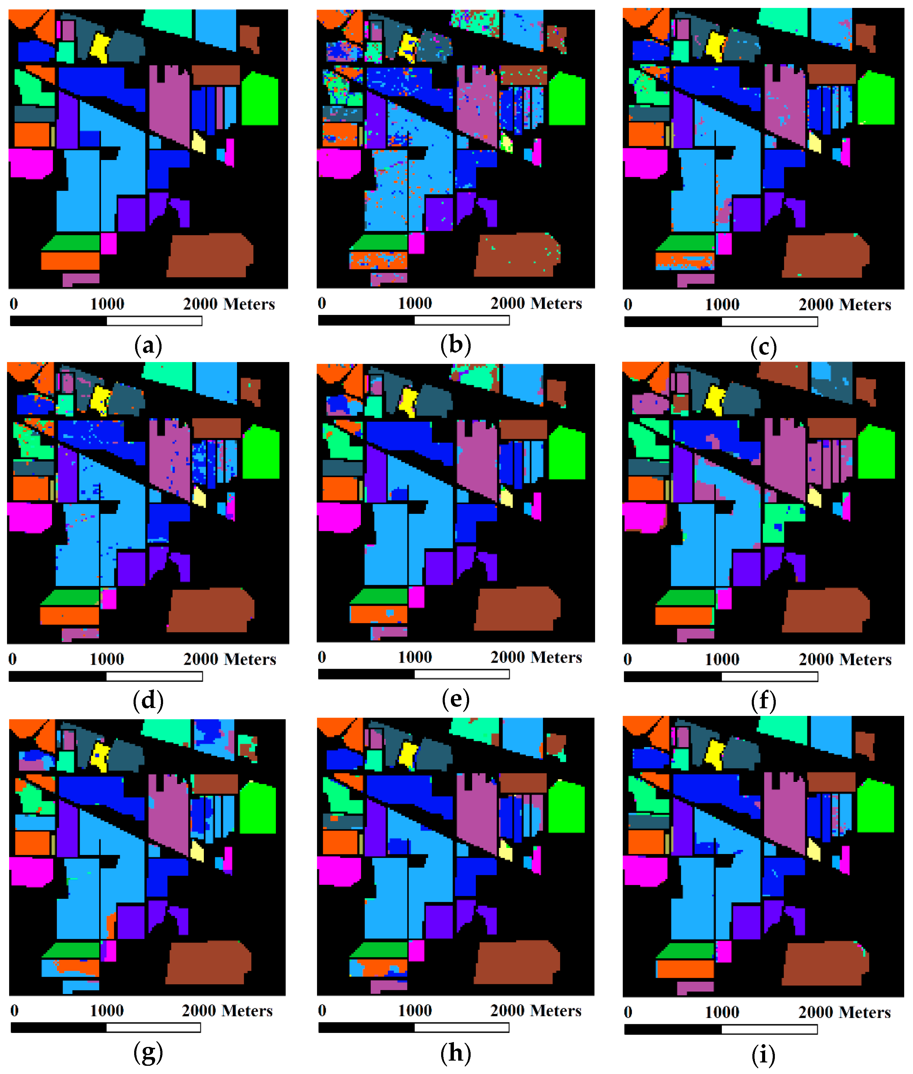
4.3. The Indian Pines Dataset

To compare our method with the other classification methods, the default parameter settings for the STK method were fixed as $\mu =0.8$ and $nb\_seg=170$. The optimal parameter settings of the SVM classifier used by the other classification methods with a Gaussian RBF kernel were obtained by a fivefold cross validation: $C=2084$, $\gamma =2$. The reference data and the resultant classification maps achieved by different classification techniques are demonstrated in Figure 3a–i. It can be observed from Figure 3b that the classification map obtained by the standard SVM classifier was severely contaminated with salt-and-pepper class noise, because that this method only used spectral information to distinguish different land covers in hyperspectral images, which is a common drawback of the pixel-wise classifiers. The noise was alleviated by the SSK and EMP methods as shown in Figure 3c,d, but its effect cannot thoroughly avoided by these methods, especially at the top-left of the figures. Meanwhile, misclassified regions can be observed in the classification maps obtained by the EPF-B and the LBP-AL methods. Specifically, in Figure 3e, one region of Corn-no till at the bottom-left of the image was mistakenly classified by the EPF-B method to Corn-min till, Soybeans-no till and Soybeans-min till, while the same region was misclassified by the LBP-AL method to Soybeans-no till and Soybeans-min till. In addition, one region of Bldg-Grass-Trees-Drives at the top of Figure 3e was mixed up with small-scale regions of Woods as well. The LBP-AL method cannot well differentiate the class of Soybeans-min till from Soybeans-clean till and Soybeans-no till, as shown on the left and at the bottom-left of the image in Figure 3g. Several classification errors arising from the use of the MLR-LORSAL method are shown in Figure 3f. For instance, at the top of the image, regions belonging to the classes of Corn-no till, Bldg-Grass-Trees-Drives and Soybeans-min till according to the reference data, were incorrectly classified to Soybeans-no till, Woods and Soybeans-clean till, respectively. At the center of the image, one region which should belong to Corn-no till was assigned to Corn as well. The classification map obtained by the LORSAL-AL-MLL method was better than the methods mentioned above. However, it misclassified some regions of Corn-min till to Soybeans-min till and Corn-no till, as shown at the bottom-left in Figure 3h and cannot precisely discriminate objects in homogeneous and near-edge regions. Although the state-of-the-art spectral-spatial classification methods, such as the SSK, EMP, EPF-B and LORSAL-AL-MLL methods, can achieve visually smoother maps by incorporating spatial information with spectral features, these methods failed in some particular regions and edges, as mentioned above. In contrast, our method is capable of discriminating various features between different objects and removing differentiation among the same category simultaneously. Therefore, it can carry out much smoother homogeneous regions and more accurate classification results for object boundaries, as shown in Figure 3i.

To objectively evaluate the performance of our method, the classification accuracies obtained by all the classification methods for comparison are listed in

Table 2. The GAs and CAs (in %) for the Indian Pines image by all the classification methods for comparison. The highest accuracies are indicated in bold in each category.

Class	SVM	SSK	EMP	EPF-B	MLR-LORSAL	LBP-AL	LORSAL-AL-MLL	STK
Alfalfa	81.82	86.36	88.64	81.82	93.18	97.73	93.18	100
Corn-no till	76.61	91.01	83.35	88.77	37.80	79.63	97.06	95.74
Corn-min till	72.7	82.29	95.07	91.74	83.62	85.09	87.22	98.54
Corn	46.45	91.94	82.46	94.79	99.53	80.57	97.16	97.63
Grass/pasture	86.16	94.87	87.95	97.32	82.37	87.95	94.87	95.54
Grass/trees	89.75	98.07	96.88	98.66	97.03	100	100	98.07
Grass/pasture-mowed	87.5	100	100	100	100	93.75	100	100
Hay-windrowed	97.28	99.09	99.09	100	99.32	99.09	99.09	99.32
Oats	100	100	100	100	100	100	100	100
Soybeans-no till	83.03	90.02	90.37	86.70	98.74	78.9	92.43	95.30
Soybeans-min till	87.62	93.74	98.02	98.74	76.42	89.65	96.04	98.56
Soybeans-clean till	66.55	93.67	80.11	99.28	97.65	72.33	93.13	95.30
Wheat	96.34	98.95	98.95	100	99.48	100	100	98.95
Woods	93.3	99.57	99.83	99.66	100	94.59	97.94	99.14
Bldg-Grass-Trees-Drives	61.4	98.53	96.78	72.51	4.09	97.95	88.89	98.54
Stone-steel towers	63.53	97.65	95.29	89.41	100	94.12	84.71	100
OA	82.51	93.69	93.24	94.61	79.51	87.99	95.31	97.61
AA	80.63	94.74	93.30	93.71	85.58	90.71	95.11	98.16
κ	79.96	92.81	92.27	93.84	76.97	86.23	94.64	97.27

. It can be seen from this table that the highest OA, AA and κ were achieved by our method with 97.61%, 98.16% and 97.7%, which is a marked increase of 15.1%, 17.53% and 17.31%, respectively, compared to the pixel-wise SVM classifier. Although the highest CAs for only 6 of 16 classes were achieved when using the STK method, all of the CAs obtained by our method in Table 2 were higher than 95%. Therefore, our method can produce more reliable classification maps with high classification accuracies.

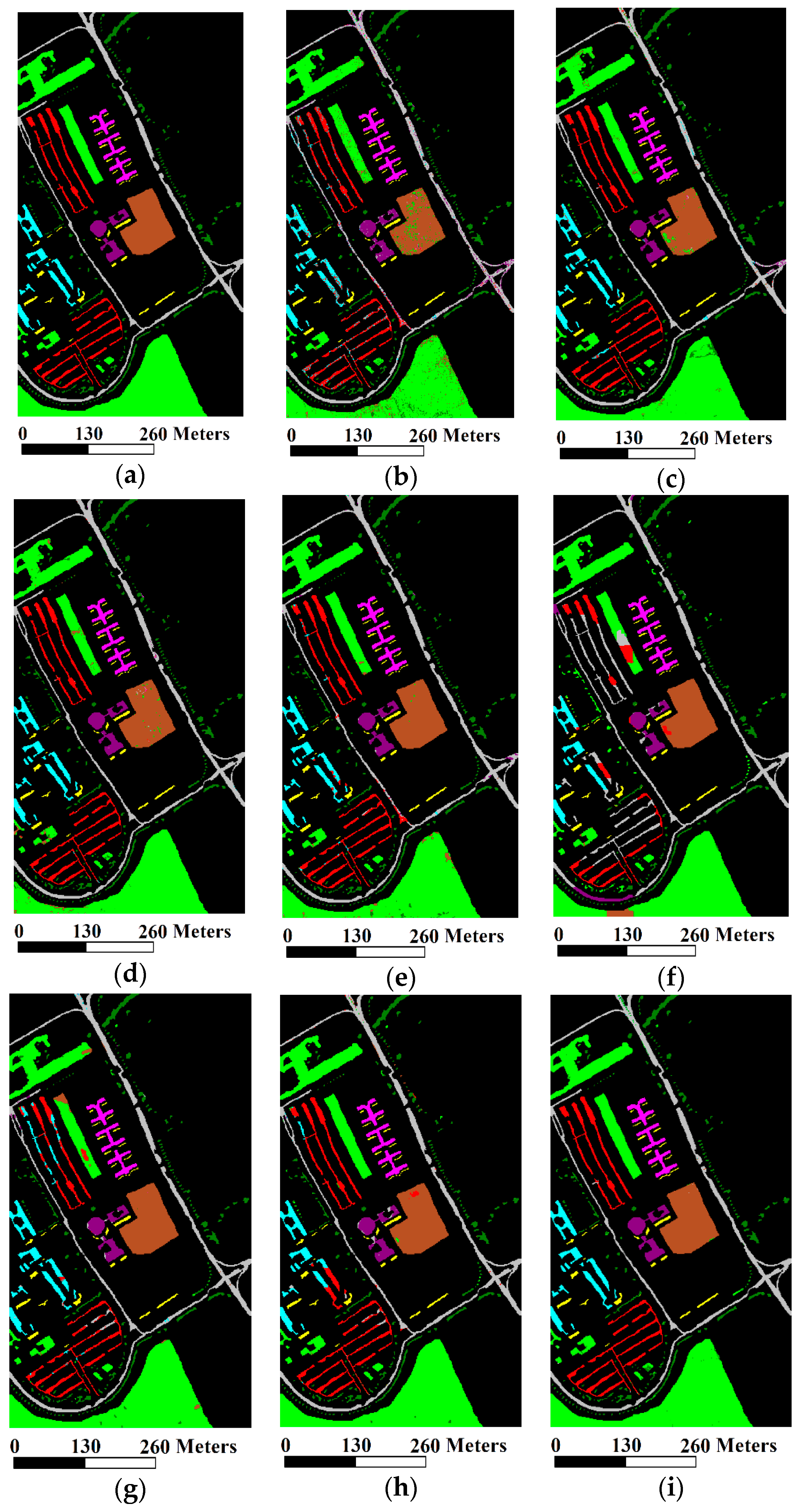
4.4. The University of Pavia Dataset

To compare our method with the other classification methods, the default parameter settings for the STK method were fixed as $\mu =0.8$ and $nb\_seg=90$. The optimal parameters of the SVM classifier used by the other classification methods with a Gaussian RBF kernel were obtained by a fivefold cross validation: $C=2048$, $\gamma =2$. The classification maps obtained by different methods and the corresponding classification accuracies are shown in Figure 4 and

Table 3. The GAs and CAs (in %) for the University of Pavia image by all the classification methods for comparison. The highest accuracies are indicated in bold in each category.

Class	SVM	SSK	EMP	EPF-B	MLR-LORSAL	LBP-AL	LORSAL-AL-MLL	STK
Asphalt	85.02	96.01	95.73	96.11	91.88	98.67	98.35	98.72
Meadows	92.26	97.6	92.96	97.75	94.42	97.14	99.79	99.34
Gravel	84.32	96.85	97.59	95.57	70.87	96.81	77.48	100
Trees	97.58	94.19	98.90	98.65	80.49	98.47	95.16	95.62
Metal Sheets	99.73	99.92	100	99.82	99.92	99.73	99.84	100
Bare Soil	91.88	96.47	88.10	99.73	98.14	99.96	98.21	99.74
Bitumen	93.24	98.81	99.52	98.61	90.16	95.95	92.62	100
Self-Blocking Bricks	85.23	96.96	98.06	96.42	44.99	81.67	93.66	99.34
Shadow	100	99.89	99.54	100	100	99.28	99.89	100
OA	90.85	97.04	94.45	97.69	88.26	96.55	97.24	99.11
AA	92.14	97.41	96.71	98.07	85.65	96.37	94.99	99.20
κ	87.81	96.07	92.67	96.89	84.36	95.35	96.32	98.82

, respectively. We can observe from Figure 4b that the classification map obtained by the pixel-wise SVM classifier contained a lot of salt-and-pepper class noise, which cannot be thoroughly avoided by the SSK, EMP and EPF_B methods, especially for the noise in the classes of Meadows and Bare Soil, as shown in Figure 4c–e. In contrast, the MLR-LORSAL, LBP-AL and LORSAL-AL-MLL methods can produce much smoother classification maps, as shown in Figure 4e–g. However, there were several misclassification effects in Figure 4f caused by the MLR-LORSAL classifier. Specifically, the most of regions belonging to Self-Blocking Bricks were classified as Asphalt; one region of Gravel were classified as Self-Blocking Bricks and Asphalt. In the resultant map in Figure 4g, several regions belonging to Self-Blocking Bricks were classified as Asphalt and Gravel by the LBP-AL method. Meanwhile, a large region (belonging to Meadows) at the bottom of Figure 4g still included small amounts of the salt-and-pepper noise. It can be seen from Figure 4g that two regions of Gravel were classified as Self-Blocking Bricks. The salt-and-pepper class noise can be observed in two regions at the bottom and at the center of the classification map in Figure 4h as well. Finally, the classification map in Figure 4i obtained by our method was highly close to the reference data in Figure 2d, except very few misclassification effects in two regions, at the center and at the lower of Figure 4i, belonging to Bare Soil and Meadows, respectively.

The classification accuracies obtained by all the classification methods for comparison are listed in Table 3. From this table, it can be seen that the GAs achieved by our method were better than the other methods. The highest OA, AA, and kappa in Table 3 were obtained by the STK method, showing increases of 8.26%, 7.07%, and 11.01%, respectively, compared to the pixel-wise SVM classifier. Meanwhile, the highest CAs for 6 of 9 classes were achieved when using the STK method, i.e., Asphalt, Gravel, Metal Sheets, Bitumen, Self-Blocking Bricks and Shadow. Moreover, all of the CAs obtained by our method in Table 3 were better than 95%. As a consequence, the STK method is superior to the other classification methods for hyperspectral images.

5. Discussion

5.1. Influence of Parameters

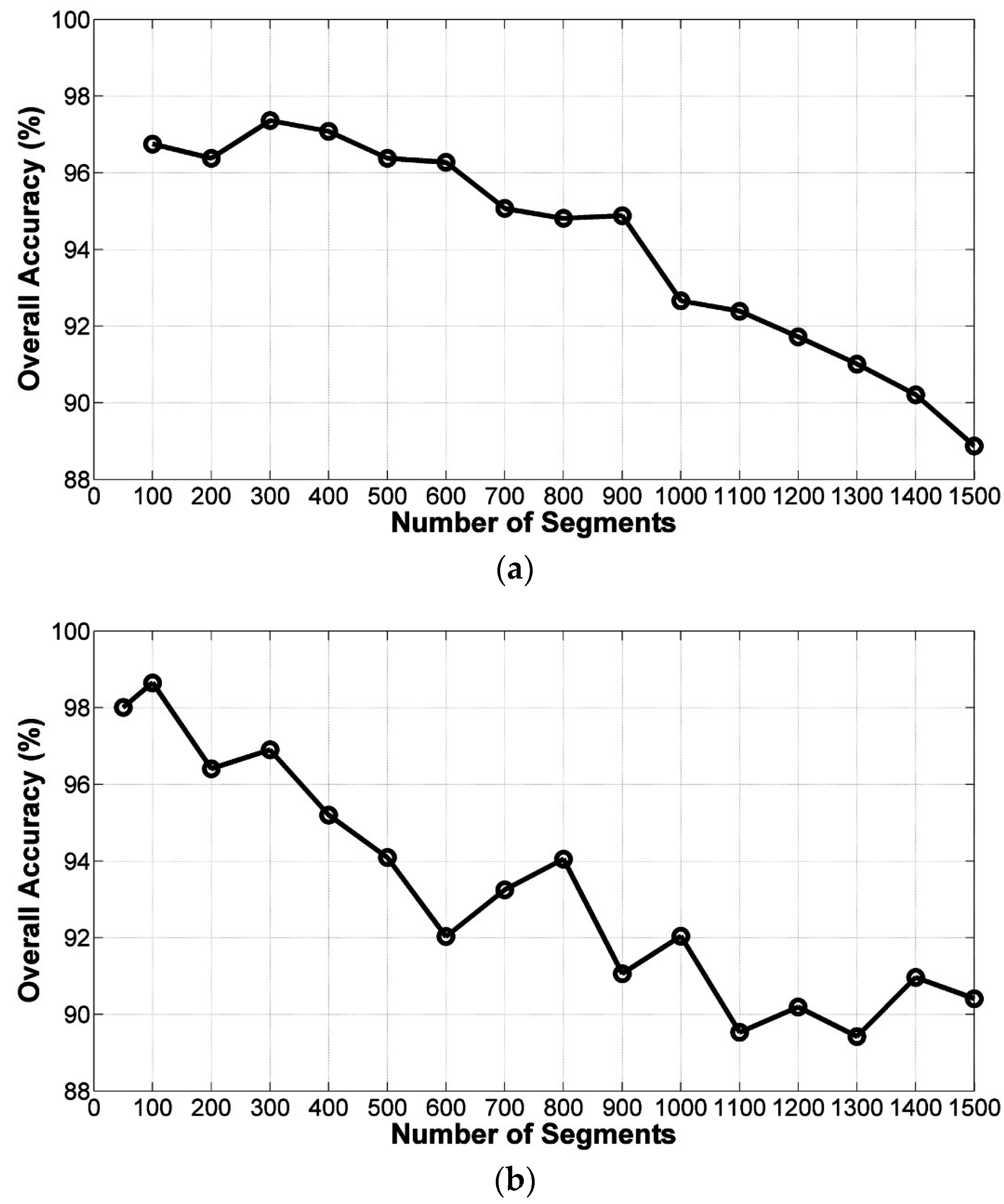
(1) Influence of nb_seg

In this subsection, the influence of partitioned regions obtained by the ERS technique to the performance of our method is first analyzed. Experiments were performed on two datasets, i.e., the Indian Pines dataset and the University of Pavia dataset. The training-test samples for each dataset and the default parameter settings of the STK method were fixed the same as the previous experiments in Section 4. Figure 5 describes the evolution of the OA obtained by the STK method with different number of segments increased from 100 to 1500 for the Indian Pines image and 50 to 1500 for the University of Pavia image. It can be noticed from this figure that the shapes of these plots have a similar global variation, i.e., that the OA values rapidly reached to an extreme point when the number of segments nb_seg increased from 100 and 50 to 300 and 100, for the Indian Pines dataset and the University of Pavia dataset, respectively. After this maximum, the OA values indicated a decreasing tendency as the increase of nb_seg. When nb_seg is very large, the whole image is separated into many small-scale regions by the ERS method. Since the required texture features are extracted from the obtained small-scale regions, these features may fluctuate from different regions belonging to the identical class of interest. Therefore, the final OA values are always reduced. It should be noted from Figure 5b that it appeared unusual increasing fluctuation as the increase of nb_seg, which was not consistent with the global behavior mentioned above, due to the fact that the distribution of objects in the University of Pavia dataset is more complex than the Indian Pines dataset, which consists of a wide range of vegetation types. To visualize the impact of nb_seg on the classification performance of our method, the classification maps for the University of Pavia dataset with different values of nb_seg (100, 500, 1000, 1500) are shown in Figure 6. We obtain a very satisfactory classification map with the highest OA of 98.65% if nb_seg = 100. As nb_seg is increased, more and more misclassification effects occurred in the classification maps, especially in Meadows at the bottom and Bare Soil at the center of the image. It can be concluded from Figure 6 that nb_seg cannot be set too large because many small miscellaneous components may be misclassified as different land covers in the homogeneous regions.

Based on the above analyses, for classification of unlabeled data, nb_seg should be a data-dependent parameter. (i) If the unlabeled data are spatially and spectrally close like the Indian Pines data set, i.e., the unlabeled data contains more different types of ground objects and the distribution of those objects in the unlabeled data is unbalanced, a large value of nb_seg is recommended to effectively discriminate the small-scale objects, e.g., $nb\_seg=300$; (ii) If the unlabeled data mainly contains the ground objects with quite regular boundaries and the distribution of all the ground objects is relatively uniform, nb_seg can be set as a relatively small value to obtain satisfactory results, e.g., $nb\_seg=50$; (iii) If there is no prior knowledge, considering the classification performance, we recommend selecting a relatively moderate value of nb_seg as $nb\_seg=100$.

Since image pixels in each homogeneous region have similar texture features, it is more accurate to perform the local spectral histogram model in those homogeneous regions. Meanwhile, it is not necessary for our method to select an optimal integration scale, which was defined in the original work of [36,38] as the window size used to compute local spectral histogram features. To demonstrate the effectiveness of our method, we applied the STK method using different fixed-size windows for texture extraction and our method using the ERS algorithm for texture extraction on the University of Pavia dataset, and the corresponding classification accuracies are listed in

Table 4. Classification accuracy (%) achieved by the STK method using different integration scales and our method on the University of Pavia dataset. The highest accuracies are indicated in underlined in each category.

Method	Integration Scale	Classification Accuracy (%)
		OA	AA	κ
STK	15 × 15	93.15	94.26	90.94
	25 × 25	96.34	97.2	95.14
	35 × 35	97.17	97.8	96.24
	45 × 45	97.6	98.05	96.81
	55 × 55	97.67	98.18	96.91
	65 × 65	98.2	98.51	97.64
	75 × 75	98.16	98.49	97.55
	85 × 85	97.84	98.18	97.12
STK		99.11	99.2	98.82

. The training-test samples for this dataset and the default parameter settings of the STK method were fixed the same as the previous experiments in Section 4. It can be observed from this table that the classification accuracies achieved by our method are higher than the STK method using different integration scales. Therefore, our method results in improved classification accuracy.

(2) Influence of μ

Then, the influence of the weight μ in the spectral-texture kernel in Equation (12) to the performance of our method is analyzed. Experiments were performed on two datasets, i.e., the Indian Pines dataset and the University of Pavia dataset. The training-test samples for each dataset and the default parameter settings of the STK method were fixed the same as the previous experiments in Section 4. Figure 7 depicts the classification results obtained by our method using different values of μ from 0 to 1 with a step size of 0.1. It can be seen in Figure 7 that our method can greatly improve classification accuracies by integrating spectral information with texture information in the classification process. For instance, the classification accuracies by our method varying μ from 0.1 to 0.9 is much higher than the conventional SVM classifier only with the spectral kernel ($\mu =0$) in Equation (11) or the texture kernel ($\mu =1$) in Equation (13). For the Indian Pines dataset, the OA obtained by our method increased from 87.61% ($\mu =0$) to over 97% and decreased to 95.3% ($\mu =1$); for the University of Pavia dataset, the OA obtained by our method increased from 87.4% ($\mu =0$) to over 99% and dropped to 82.17% ($\mu =1$). Moreover, our method is not sensitive to μ because the classification accuracies by our method varying μ from 0.1 to 0.9 were highly stable. Our experiments in Section 4 confirmed that $\mu =0.8$ performs the best for the STK method on both of the two datasets. Therefore, if there is no prior knowledge, considering the classification performance, we recommend setting μ as $0.5\le \mu \le 0.9$.

(3) Influence of M

Next, the influence of M (the number of $F^{\left(\alpha \right)}$ in Section 2.2) in the spectral-texture kernel in Equation (12) to the performance of our method is analyzed. The number of the filters, which are introduced in Section 2.2, is crucial for texture extraction. To demonstrate the classification results with different values of M, we applied the STK method on the University of Pavia dataset and the default parameter settings were fixed the same as the previous experiments in Section 4.

Table 5. Classification accuracy (%) achieved by the STK method on the University of Pavia dataset using different combinations of the five filters. The highest accuracies are indicated in underlined in each category.

Filter(s)	Overall Accuracy (%)
Intensity	98.5
Two LoG filters	97.14
Two Gabor filters	95.06
Intensity + two LoG filters	99.09
Intensity + two Gabor filters	99.06
Two LoG filters + two Gabor filters	96.67
Intensity + two LoG filters + two Gabor filters	99.11

summarizes the OAs achieved by our method with different combinations of the five filters and we can observe in this Table: (1) If any type of the three filters is individually utilized to compute local spectral histogram, the STK method using the intensity filter can achieve the best OA of 98.5%; (2) If any pairs of the three types of filters are utilized, the STK method including the intensity filter can achieve considerably high OA. For instance, the OA can be higher than 99% when the “Intensity + two LoG filters” or the “Intensity + two Gabor filters” are used in the STK method. Therefore, based on the above observations, the intensity filter dominantly contributes the final classification results; (3) The highest OA can be obtained when all the filters are used in our method. Apart from the three types of filters, other filters can be used for texture extraction as well. All of our experiments on hyperspectral images, including those not reported here, confirmed that if a hyperspectral image has complex texture features and the difference among regions is small, we can achieve more accurate classification maps as the number of filters is increased.

(4) Influence of ${\sigma }_{\mathrm{LoG}}$ and ${\sigma }_{\mathrm{Gabor}}$

In the following, the influence of ${\sigma }_{\mathrm{LoG}}$ and ${\sigma }_{\mathrm{Gabor}}$ in the LoG and Gabor filters, respectively, to the performance of our method is analyzed. Experiments were performed on the two datasets, i.e., the Indian Pines dataset and the University of Pavia dataset. To analyze the influence of ${\sigma }_{\mathrm{LoG}}$, a set of ${\sigma }_{\mathrm{LoG}}$ (0.5, 1, 2, 4, 8, 16) was used in the two LoG filters; to analyze the influence of ${\sigma }_{\mathrm{Gabor}}$, we applied the STK method varying ${\sigma }_{\mathrm{Gabor}}$ from 1.5 to 5 with a step size of 0.5 in the two Gabor filters. Meanwhile, the other parameters were fixed as the previous experiments in Section 4. The corresponding OAs in terms of different parameter settings are reported in

Table 6. The impact of ${\sigma }_{\mathrm{LoG}}$ and ${\sigma }_{\mathrm{Gabor}}$ on classification accuracy for the Indian Pines and the University of Pavia datasets.

Parameter	Indian Pines		University of Pavia
	Value	OA (%)	Value	OA (%)
${\sigma }_{\mathrm{LoG}}$	0.5	97.61	0.5	99.11
	1	97.58	1	99.1
	2	97.56	2	99.1
	4	97.55	4	99.11
	8	97.53	8	99.1
	16	97.54	16	99.1
${\sigma }_{\mathrm{Gabor}}$	1.5	97.61	1.5	99.11
	2	97.6	2	99.14
	2.5	97.63	2.5	98.99
	3	97.6	3	99.15
	3.5	97.57	3.5	99.16
	4	97.58	4	99.11
	4.5	97.54	4.5	99.09
	5	97.55	5	98.59

. It can be observed that our method is not sensitive to particular choices of ${\sigma }_{\mathrm{LoG}}$ and ${\sigma }_{\mathrm{Gabor}}$. For conciseness, the default parameters of ${\sigma }_{\mathrm{LoG}}$ and ${\sigma }_{\mathrm{Gabor}}$ in the STK method were fixed as ${\sigma }_{\mathrm{LoG}}=0.5$ and ${\sigma }_{\mathrm{Gabor}}=1.5$.

(5) Influence of C and ${\sigma }_{\mathrm{STK}}$

Finally, the influence of C and ${\sigma }_{\mathrm{STK}}$ in the SVM classifier with the RBF kernel to the performance of our method is analyzed. Experiments were performed on the two datasets, i.e., the Indian Pines dataset and the University of Pavia dataset. It should be noted that the optimal C and ${\sigma }_{\mathrm{STK}}$ can be estimated using the cross validation method. For conciseness and efficiency, we defined by experience the ranges of the two parameters and selected the optimal parameter settings. To analyze the influence of C, we applied the STK method varying C from 50 to 300 with a step size of 50, while ${\sigma }_{\mathrm{STK}}$ was set to 0.5; to analyze the influence of ${\sigma }_{\mathrm{STK}}$, a set of ${\sigma }_{\mathrm{STK}}$ (0.2, 0.5, 1, 1.5, 2, 2.5, 3) was used in the SVM classifier while C was fixed as 200. Meanwhile, the other parameters in our method were fixed as the previous experiments in Section 4. The corresponding OAs in terms of different parameter settings are listed in

Table 7. The impact of C and ${\sigma }_{\mathrm{STK}}$ on classification accuracy for the Indian Pines and the University of Pavia datasets. The highest accuracies are indicated in underlined in each category.

Parameter	Indian Pines		University of Pavia
	Value	OA (%)	Value	OA (%)
C	50	97.43	50	98.01
	100	97.53	100	98.91
	150	97.58	150	99.12
	200	97.61	200	99.11
	250	97.57	250	99.1
	300	97.57	300	99.1
${\sigma }_{\mathrm{STK}}$	0.2	97.39	0.2	98.24
	0.5	97.61	0.5	99.11
	1	97.46	1	98.66
	1.5	97.37	1.5	98.46
	2	97.31	2	98.48
	2.5	97.25	2.5	98.44
	3	97.2	3	98.44

. It can be seen from this table that our method can achieve the highest OA of 97.61% using the optimal parameter settings of $C=200$ and ${\sigma }_{\mathrm{STK}}=0.5$ for the Indian Pines dataset. In addition, our method can obtain the OA around 99.11% with C ranging from 150 to 300 while ${\sigma }_{\mathrm{STK}}=0.5$, for the University of Pavia dataset. Therefore, based on our experiments on hyperspectral data, including those not reported here, our method is not very sensitive to the penalty term C and ${\sigma }_{\mathrm{STK}}$. Even though the selected C and ${\sigma }_{\mathrm{STK}}$ may be not optimal, our method can effectively improve classification performance of hyperspectral data in terms of visual inspection and classification accuracies. For conciseness, we recommend fixing the values of C and ${\sigma }_{\mathrm{STK}}$ as $C=200$ and ${\sigma }_{\mathrm{STK}}=0.5$.

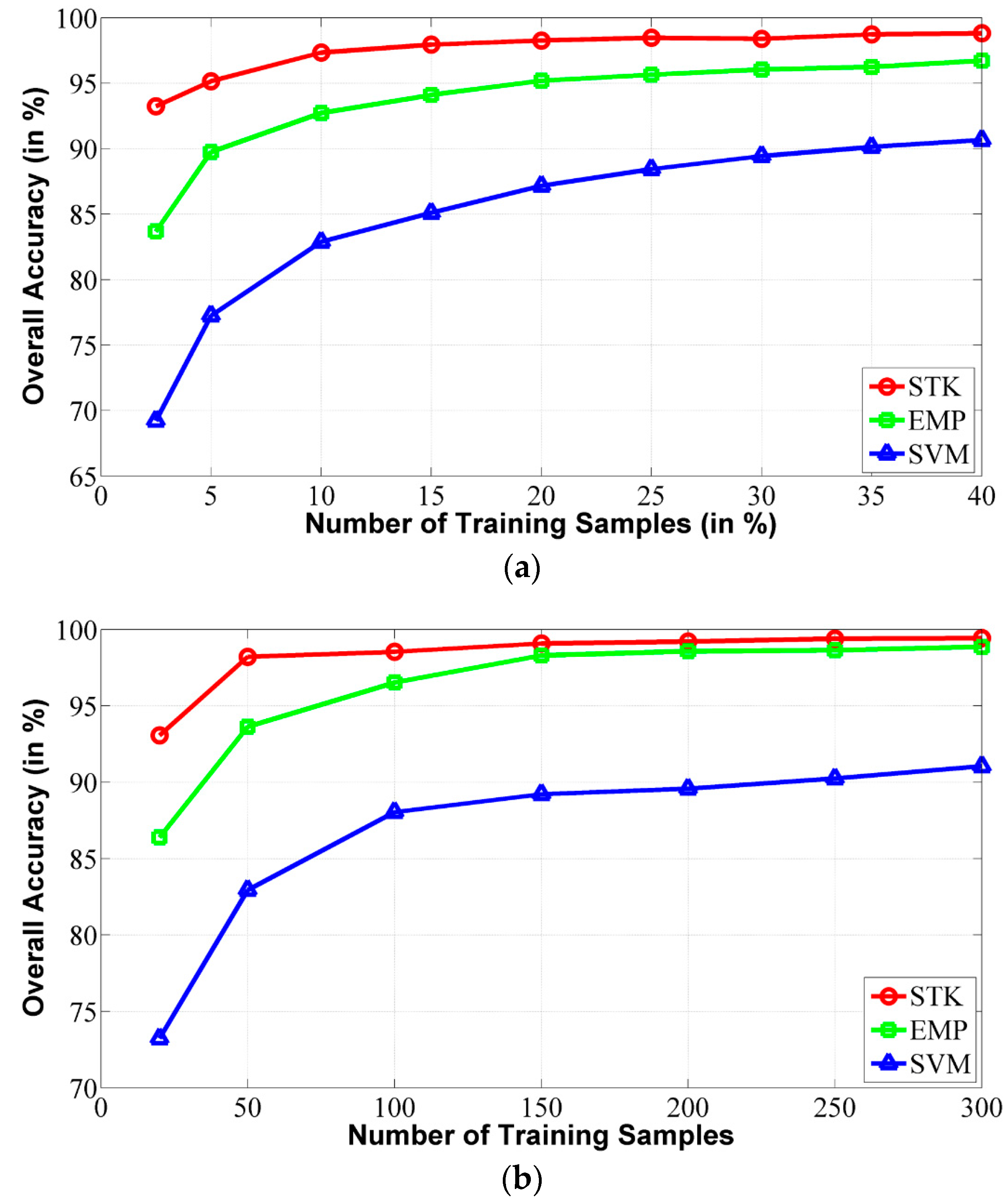
5.2. Classification Results with Different Number of Training Samples

In this subsection, the influence of different number of training samples to the stability of the STK method is analyzed. Experiments were performed on the Indian Pines dataset and the University of Pavia dataset. In our experiments, the SVM, EMP and STK methods were used for comparison and the default parameter settings of these methods were fixed the same as the previous experiments in Section 4. The number of training samples for each class used by these methods increased from 2.5% to 40% for the Indian Pines image. Regarding the University of Pavia, the number of training samples for each class was set from 25 to 300. To accurately obtain the classification results, the OA values obtained by the three methods with different training samples were the average results over five trials. Figure 8 illustrates the evolution of the OA obtained by the STK method with different number of training samples for the two hyperspectral datasets. It can be noticed from this figure that the OA values achieved by the three classification methods were positively correlated with the number of training samples. Meanwhile, the STK method outperformed the other two methods with the same number of training samples for all of the two hyperspectral datasets. Moreover, our method can demonstrate outstanding performance in terms of the OA values when the number of training samples is considerably limited. For instance, with respect to the Indian Pines image, our method can obtain the OA value of 93.24% when the number of training samples is only 2.5% of the reference data. In contrast, it required more than 10% of the reference data for training for the EMP method to achieve an OA value higher than 93.24%. Moreover, the OA values obtained by the SVM method was much lower than that of our method, no matter how many training samples were used for classification. Regarding the University of Pavia image, it can be observed that, with only 50 training samples for each class (over 1% of the reference data), the STK method can obtain an OA value of 98.21%, which were much higher than that of the other two methods.

5.3. Classification Results with Different Number of PCA Components

In this subsection, the influence of different number of PCA components to the performance of the STK method is analyzed using the two hyperspectral datasets used in the previous section. To provide further insights with respect to the most appropriate PCA components, three combinations of those components were considered in the STK method for the extraction of texture features as follows:

(1)

The first component (PC1) which corresponds to the highest eigenvalue and contains the most abundant data information;

(2)

The first two components (PC1 + PC2);

(3)

The first three components (PC1 + PC2 + PC3).

The default parameter settings of our method were fixed the same as the previous experiments in Section 4 and the classification accuracies achieved by our method with the three combinations of the PCA components are listed in

Table 8. Classification accuracy (%) of the STK method with different number of the PCA components for the Indian Pines and University of Pavia datasets.

Option	Classification Accuracy
	Indian Pines			University of Pavia
	OA	AA	κ	OA	AA	κ
PC1	97.61	98.16	97.27	99.11	99.2	98.82
PC1 + PC2	97.63	98.19	97.29	99.13	99.24	99.84
PC1 + PC2 + PC3	97.64	98.2	97.31	99.14	99.24	99.85

. As the number of the PCA components is increased, the classification accuracies can be improved by the STK method as shown in Table 8, but those improvements are very limited. Specifically, the proposed method with PC1 + PC2 and PC1 + PC2 + PC3 can achieve improvements of 0.02% and 0.03% in terms of OA over our method only with PC1 for both of the two hyperspectral datasets, respectively. For conciseness and efficiency, the first component was used in the STK method for texture extraction.

5.4. Running Time Comparison for Different Approaches

In this subsection, the computational complexity of the STK method is analyzed and several classification methods, including SVM, EMP, MLR-LORSAL and LORSAL-AL-MLL, were used for comparison. All the reported experiments were performed using a MATLAB program on Microsoft Windows 7 running on a PC with 3.4 GHz, Intel Core i3-2130 processor and 4GB of RAM. It should be noted that our source code is not optimal in the sense that we make it an intermediate step to a final code in C++. To objectively evaluate the efficiency of each method used here, we can measure the mean of five executions for comparison. The computational times of different classification methods on the two hyperspectral datasets are listed in

Table 9. Efficiency of different classification methods of the SVM, EMP, MLR-LORSAL, LORSAL-AL-MLL and STK methods for the Indian Pines and University of Pavia datasets.

Method	Time Used (s)
	Indian Pines	University of Pavia
SVM	133.24	26.59
EMP	38.74	19.76
MLR-LORSAL	5.36	9.42
LORSAL-AL-MLL	211.46	170.34
STK	2.58	12.10

. It took much time for the conventional SVM classifier to search for optimal parameters using the time-consuming k-fold cross-validation step. Meanwhile, it is necessary for the LORSAL-AL-MLL method to perform an exhausted active learning step during the classification process. With respect to the EMP method, the production of EMPs is not a very efficient process as well. Although the speed of the MLR-LORSAL method can be comparable with our method, the misclassification effects always occurred in the resultant maps by the MLR-LORSAL method as described in Section 4, which greatly reduced classification accuracies. In our algorithm, the ERS segmentation process and the local spectral histograms calculation are two efficient steps. Therefore, our method is much more efficient than the state-of-the-art classification methods for hyperspectral images.

6. Conclusions

In this paper, we presented a spectral-texture kernel-based classification method for hyperspectral images. The major contributions of this work are twofold: First, a region-based spectral histogram technique was introduced as an effective tool for texture representation, which can describe texture features in hyperspectral images in a more accurate manner, compared to the conventional methods. Second, a composite kernel was constructed by combining both spectral information and the extracted texture information characterized by the region-based spectral histogram. By using the proposed spectral-texture kernel, our method can effectively improve classification accuracies of hyperspectral images, even though only a very limited training samples is available. The proposed STK method was compared with other state-of-the-art classification methods using objective quantitative measures and a visual qualitative evaluation. Experimental results on the two airborne hyperspectral datasets confirmed that our method was better than the other methods in terms of the GAs. For instance, the STK method can obtain improvements of 15.1% and 8.26% in terms of OA over the conventional SVM classifier for the Indian Pines dataset and the University of Pavia dataset, respectively. Furthermore, for both of the two datasets, the STK method can obtain the highest classification accuracies among all of the classification methods. In addition, the proposed STK method was robust relative to the parameters and the choice of those parameters was carefully analyzed. In the future, a further improvement will be achieved by investigating more efficient texture extraction approaches.

References

1. Plaza, A.; Benediktsson, J.A.; Boardman, J.W.; Brazile, J.; Bruzzone, L.; Camps-Valls, G.; Chanussot, J.; Fauvel, M.; Gamba, P.; Gualtieri, A.; et al. Recent advances in techniques for hyperspectral image processing. Remote Sens. Environ. 2009, 113, S110–S122. [Google Scholar] [CrossRef]
2. Camps-Valls, G.; Tuia, D.; Bruzzone, L.; Benediktsson, J.A. Advances in hyperspectral image classification: Earth monitoring with statistical learning methods. IEEE Signal Peocess. Mag. 2014, 31, 45–54. [Google Scholar] [CrossRef]
3. Hughes, G. On the mean accuracy of statistical pattern recognizers. IEEE Trans. Inf. Theory 1968, 14, 55–63. [Google Scholar] [CrossRef]
4. Landgrebe, D.A. Signal Theory Methods in Multispectral Remote Sensing; Wiley-Interscience: Hoboken, NJ, USA, 2003. [Google Scholar]
5. Chen, C.H.; Peter Ho, P.-G. Statistical pattern recognition in remote sensing. Pattern Recognit. 2008, 41, 2731–2741. [Google Scholar] [CrossRef]
6. Ham, J.; Chen, Y.; Crawford, M.M.; Ghosh, J. Investigation of the random forest framework for classification of hyperspectral data. IEEE Trans. Geosci. Remote Sens. 2005, 43, 492–501. [Google Scholar] [CrossRef]
7. Ratle, F.; Camps-Valls, G.; Weston, J. Semisupervised neural networks for efficient hyperspectral image classification. IEEE Trans. Geosci. Remote Sens. 2010, 48, 2271–2282. [Google Scholar] [CrossRef]
8. Yang, H. A back-propagation neural network for mineralogical mapping from AVIRIS data. Int. J. Remote Sens. 1999, 20, 97–110. [Google Scholar] [CrossRef]
9. Melgani, F.; Bruzzone, L. Classification of hyperspectral remote sensing images with support vector machines. IEEE Trans. Geosci. Remote Sens. 2004, 42, 1778–1790. [Google Scholar] [CrossRef]
10. Bennett, K.P.; Demiriz, A. Semi-supervised support vector machines. In Proceedings of the 1998 Conference on Advances in Neural Information Processing Systems II; MIT Press: Denver, CO, USA, 1999; pp. 368–374. [Google Scholar]
11. Moustakidis, S.; Mallinis, G.; Koutsias, N.; Theocharis, J.B.; Petridis, V. SVM-based fuzzy decision trees for classification of high spatial resolution remote sensing images. IEEE Trans. Geosci. Remote Sens. 2012, 50, 149–169. [Google Scholar] [CrossRef]
12. Camps-Valls, G.; Bruzzone, L. Kernel Methods for Remote Sensing Data Analysis; Wiley: New York, NY, USA, 2009. [Google Scholar]
13. Camps-Valls, G.; Marsheva, T.V.B.; Zhou, D. Semi-supervised graph-based hyperspectral image classification. IEEE Trans. Geosci. Remote Sens. 2007, 45, 3044–3054. [Google Scholar] [CrossRef]
14. Fauvel, M.; Tarabalka, Y.; Benediktsson, J.A.; Chanussot, J.; Tilton, J.C. Advances in spectral-spatial classification of hyperspectral images. Proc. IEEE 2013, 101, 652–675. [Google Scholar] [CrossRef]
15. Zhang, Y. Optimisation of building detection in satellite images by combining multispectral classification and texture filtering. ISPRS J. Photogramm. Remote Sens. 1999, 54, 50–60. [Google Scholar] [CrossRef]
16. Huang, X.; Zhang, L. A comparative study of spatial approaches for urban mapping using hyperspectral rosis images over Pavia City, northern Italy. Int. J. Remote Sens. 2009, 30, 3205–3221. [Google Scholar] [CrossRef]
17. Benediktsson, J.A.; Palmason, J.A.; Sveinsson, J.R. Classification of hyperspectral data from urban areas based on extended morphological profiles. IEEE Trans. Geosci. Remote Sens. 2005, 43, 480–491. [Google Scholar] [CrossRef]
18. Mura, M.D.; Villa, A.; Benediktsson, J.A.; Chanussot, J.; Bruzzone, L. Classification of hyperspectral images by using extended morphological attribute profiles and independent component analysis. IEEE Geosci. Remote Sens. Lett. 2011, 8, 542–546. [Google Scholar] [CrossRef]
19. Shen, L.; Zhu, Z.; Jia, S.; Zhu, J.; Sun, Y. Discriminative Gabor feature selection for hyperspectral image classification. IEEE Geosci. Remote Sens. Lett. 2013, 10, 29–33. [Google Scholar] [CrossRef]
20. Chen, C.; Li, W.; Su, H.; Liu, K. Spectral-spatial classification of hyperspectral image based on kernel extreme learning machine. Remote Sens. 2014, 6, 5795–5814. [Google Scholar] [CrossRef]
21. Li, J.; Bioucas-Dias, J.M.; Plaza, A. Spectral-spatial hyperspectral image segmentation using subspace multinomial logistic regression and Markov random fields. IEEE Trans. Geosci. Remote Sens. 2012, 50, 809–823. [Google Scholar] [CrossRef]
22. Xia, J.; Chanussot, J.; Du, P.; He, X. Spectral-spatial classification for hyperspectral data using rotation forests with local feature extraction and Markov random fields. IEEE Trans. Geosci. Remote Sens. 2015, 53, 2532–2546. [Google Scholar] [CrossRef]
23. Camps-Valls, G.; Gomez-Chova, L.; Munoz-Mari, J.; Vila-Frances, J.; Calpe-Maravilla, J. Composite kernels for hyperspectral image classification. IEEE Geosci. Remote Sens. Lett. 2006, 3, 93–97. [Google Scholar] [CrossRef]
24. Mathieu, F.; Jocelyn, C.; Atli, B.J. A spatial–spectral kernel-based approach for the classification of remote-sensing images. Pattern Recognit. 2012, 45, 381–392. [Google Scholar]
25. Camps-Valls, G.; Shervashidze, N.; Borgwardt, K.M. Spatio-spectral remote sensing image classification with graph kernels. IEEE Geosci. Remote Sens. Lett. 2010, 7, 741–745. [Google Scholar] [CrossRef]
26. Tarabalka, Y.; Chanussot, J.; Benediktsson, J.A. Segmentation and classification of hyperspectral images using watershed transformation. Pattern Recognit. 2010, 43, 2367–2379. [Google Scholar] [CrossRef]
27. Huang, X.; Zhang, L. An adaptive mean-shift analysis approach for object extraction and classification from urban hyperspectral imagery. IEEE Trans. Geosci. Remote Sens. 2008, 46, 4173–4185. [Google Scholar] [CrossRef]
28. Ghamisi, P.; Couceiro, M.S.; Fauvel, M.; Benediktsson, J.A. Integration of segmentation techniques for classification of hyperspectral images. IEEE Geosci. Remote Sens. Lett. 2014, 11, 342–346. [Google Scholar] [CrossRef]
29. Tarabalka, Y.; Tilton, J.C.; Benediktsson, J.A.; Chanussot, J. A marker-based approach for the automated selection of a single segmentation from a hierarchical set of image segmentations. IEEE J. Sel. Top. Appl. Earth Obs. Remote Sens. 2012, 5, 262–272. [Google Scholar] [CrossRef]
30. Song, H.; Wang, Y. A spectral-spatial hyperspectral image classification based on algebraic multigrid methods and hierarchical segmentation. Remote Sens. 2016, 8, 296. [Google Scholar] [CrossRef]
31. Fang, L.; Li, S.; Kang, X.; Benediktsson, J.A. Spectral-spatial classification of hyperspectral images with a superpixel-based discriminative sparse model. IEEE Trans. Geosci. Remote Sens. 2015, 53, 4186–4201. [Google Scholar] [CrossRef]
32. Kettig, R.L.; Landgrebe, D.A. Classification of multispectral image data by extraction and classification of homogeneous objects. IEEE Trans. Geosci. Electron. 1976, 14, 19–26. [Google Scholar] [CrossRef]
33. Tarabalka, Y.; Chanussot, J.; Benediktsson, J.A. Segmentation and classification of hyperspectral images using minimum spanning forest grown from automatically selected markers. IEEE Trans. Syst. Man Cybern. Part B Cybern. 2010, 40, 1267–1279. [Google Scholar] [CrossRef] [PubMed]
34. Tarabalka, Y.; Rana, A. Graph-cut-based model for spectral-spatial classification of hyperspectral images. In Proceedings of the IEEE Geoscience and Remote Sensing Symposium, Quebec, QC, Canada, 13–18 July 2014.
35. Wang, Y.; Song, H.; Zhang, Y. Spectral-spatial classification of hyperspectral images using joint bilateral filter and graph cut based model. Remote Sens. 2016, 8, 748. [Google Scholar] [CrossRef]
36. Yuan, J.; Wang, D.; Li, R. Image segmentation using local spectral histograms and linear regression. Pattern Recognit. Lett. 2012, 33, 615–622. [Google Scholar] [CrossRef]
37. Liu, M.Y.; Tuzel, O.; Ramalingam, S.; Chellappa, R. Entropy rate superpixel segmentation. In Proceedings of the IEEE Conference on Computer Vision and Pattern Recognition, Colorado Springs, CO, USA, 20–25 June 2011.
38. Liu, X.; Wang, D. Image and texture segmentation using local spectral histograms. IEEE Trans. Image Process. 2006, 15, 3066–3077. [Google Scholar] [CrossRef] [PubMed]
39. Yuan, J.; Wang, D.; Li, R. Remote sensing image segmentation by combining spectral and texture features. IEEE Trans. Geosci. Remote Sens. 2014, 52, 16–24. [Google Scholar] [CrossRef]
40. Schölkopf, B.; Smola, A.J. Learning with Kernels. Support Vector Machines, Regularization, Optimization, and Beyond; MIT Press: Cambridge, MA, USA, 2002. [Google Scholar]
41. Liu, X.; Wang, D. A spectral histogram model for texton modeling and texture discrimination. Vis. Res. 2002, 42, 2617–2634. [Google Scholar] [CrossRef]
42. Camps-Valls, G.; Bruzzone, L. Kernel-based methods for hyperspectral image classification. IEEE Trans. Geosci. Remote Sens. 2005, 43, 1351–1362. [Google Scholar] [CrossRef]
43. Fauvel, M.; Chanussot, J.; Benediktsson, J.A. A spatial-spectral kernel-based approach for the classification of remote-sensing images. Pattern Recognit. 2012, 45, 381–392. [Google Scholar] [CrossRef]
44. Kang, X.; Li, S.; Benediktsson, J.A. Spectral-spatial hyperspectral image classification with edge-preserving filtering. IEEE Trans. Geosci. Remote Sens. 2014, 52, 2666–2677. [Google Scholar] [CrossRef]
45. Li, J.; Bioucas-Dias, J.M.; Plaza, A. Spectral-spatial classification of hyperspectral data using loopy belief propagation and active learning. IEEE Trans. Geosci. Remote Sens. 2013, 51, 844–856. [Google Scholar] [CrossRef]
46. Bioucas-Dias, J.M.; Figueiredo, M. Logistic Regression via Variable Splitting and Augmented Lagrangian Tools; Instituto Superior Tecnico: Lisbon, Portugal, 2009. [Google Scholar]
47. Li, J.; Bioucas-Dias, J.M.; Plaza, A. Hyperspectral image segmentation using a new Bayesian approach with active learning. IEEE Trans. Geosci. Remote Sens. 2011, 49, 3947–3960. [Google Scholar] [CrossRef]
48. Chang, C.-C.; Lin, C.-J. LIBSVM: A library for support vector machines. ACM Trans. Intell. Syst. Technol. 2011, 2. [Google Scholar] [CrossRef]
49. Wu, T.-F.; Lin, C.-J.; Weng, R.C. Probability estimates for multiclass classification by pairwise coupling. J. Mach. Learn. Res. 2004, 5, 975–1005. [Google Scholar]
50. Tadjudin, S.; Landgrebe, D. Classification of High Dimensional Data with Limited Training Samples; Purdue University: West Lafayette, IN, USA, 1998. [Google Scholar]
51. Duarte-Carvajalino, J.M.; Castillo, P.E.; Velez-Reyes, M. Comparative study of semi-implicit schemes for nonlinear diffusion in hyperspectral imagery. IEEE Trans. Image Process. 2007, 16, 1303–1314. [Google Scholar] [CrossRef] [PubMed]
52. Baumgardner, M.F.; Biehl, L.L.; Landgrebe, D.A. 220 Band AVIRIS Hyperspectral Image Data Set: June 12, 1992 Indian Pine Test Site 3; Purdue University Research Repository: West Lafayette, IN, USA, 2015. [Google Scholar] [CrossRef]
53. Holzwarth, S.; Müller, A.; Habermeyer, M.; Richter, R.; Hausold, A.; Thiemann, S.; Strobl, P. Hysens-DAIS/ROSIS imaging spectrometers at DLR. In Proceedings of the 3rd EARSeL Workshop on Imaging Spectroscopy, Herrsching, Germany, 13–16 May 2003.
Figure 1. Illustration of the proposed spectral-spatial classification method for hyperspectral images.
Remotesensing 08 00919 g001
Figure 2. Hyperspectral datasets and the corresponding reference data. (a) A three-band color composite image (bands 47, 23 and 13) of the Indian Pines dataset; (b) reference data of the Indian Pines dataset; (c) a three-band color composite image (bands 103, 56 and 31) of the University of Pavia dataset; (d) reference data of the University of Pavia dataset.
Remotesensing 08 00919 g002
Figure 3. Classification maps for the Indian Pines image using different classification techniques. (a) Reference data; (b) SVM; (c) SSK; (d) EMP; (e) EPF-B; (f) MLR-LORSAL; (g) LBP-AL; (h) LORSAL-AL-MLL; (i) STK.
Remotesensing 08 00919 g003
Figure 4. Classification maps for the University of Pavia image using different classification techniques. (a) Reference data; (b) SVM; (c) SSK; (d) EMP; (e) EPF-B; (f) MLR-LORSAL; (g) LBP-AL; (h) LORSAL-AL-MLL; (i) STK.
Remotesensing 08 00919 g004
Figure 5. Evolution of the OA against the number of segments obtained by the ERS method on different images. (a) Indian pines; (b) University of Pavia.
Remotesensing 08 00919 g005
Figure 6. Classification maps and the corresponding OAs for the University of Pavia dataset by the STK method using different value of nb_seg. (a) n b _ s e g = 100 , OA = 98 . 65 % ; (b) n b _ s e g = 500 , OA = 94 . 09 % ; (c) n b _ s e g = 1000 , OA = 92 . 04 % ; (d) n b _ s e g = 1500 , OA = 90 . 41 % .
Remotesensing 08 00919 g006
Figure 7. Analysis of the Impact of the parameter μ using the STK method for the Indian Pines and University of Pavia datasets.
Remotesensing 08 00919 g007
Figure 8. Effect of number of training samples on proposed STK, EMP and SVM methods for two hyperspectral images: (a) Indian pines; (b) University of Pavia.
Remotesensing 08 00919 g008