1. Introduction
Due to the resolution constraint of sensors, in that the instantaneous field of view (FOV) is usually larger than the land-cover objects the sensors observe [
1], the mixed pixel is a common phenomenon in remote sensing imagery acquired by moderate/low-resolution sensors. Such pixels contain more than one land-cover class and cannot simply be attributed to only one class by hard classification. Therefore, the technique of spectral unmixing has been developed to handle the mixed pixel problem by analyzing and decomposing the mixed spectra to a combination form of several single pure spectra (endmembers) [
2,
3], as well as the fraction each spectra comprises in the mixed model [
4,
5,
6,
7]. In spite of this, the outputs of the spectral unmixing still retain a coarse spatial resolution, which cannot meet the requirement for detailed information.
Thus, the sub-pixel mapping method has been proposed to further improve the unmixing result by not only determining the proportion of each land-cover class within the mixed pixel, but also the specific distribution of each land-cover class, with the unmixing output as the input, generating a fine spatial resolution land-cover map. Sub-pixel mapping is based on the spatial dependence assumption, i.e., pixels which are nearer are more likely to be the same land-cover class than pixels which are further apart [
8]. This idea was derived from the First Law of Geography, proposing the idea that everything is related to everything else, but near things are more related than distant things. It has also been proved to be an effective assumption for sub-pixel mapping techniques [
9,
10]. The goal is to maximize the spatial dependence and find the most plausible sub-pixel distribution, subsequently improving the spatial resolution relative to the input coarse image. In the past decades, sub-pixel mapping algorithms have been widely developed. An early sub-pixel mapping method was direct neighboring sub-pixel mapping (DNSM) [
11], which is a simple and effective way of reconstructing a more accurate land-cover map than the traditional hard classification. Mertens et al. [
9] proposed the spatial attraction sub-pixel mapping (SASM) method considering the spatial dependence between pixels and sub-pixels, and substantially enhanced the accuracy of the reconstructed map. Atkinson et al. [
10,
12,
13,
14,
15] proposed the pixel swapping algorithm (PSSM) to maximize the spatial dependence by swapping the sub-pixels within a coarse pixel. However, only the spatial dependence between sub-pixels is taken into consideration, and the blind interactive swap just increases the computational complexity. More recently, Hopfield neural networks (HNNs) [
16,
17,
18,
19], particle swarm optimization [
20], Markov random fields [
21,
22,
23,
24,
25], the back-propagation neural network (BPSM) [
26,
27,
28,
29,
30], multiagent system [
31], and maximum a posteriori estimation [
32,
33,
34] have been proposed to solve the problem, and have improved the reconstruction result compared to the traditional methods. Nevertheless, most of the current sub-pixel mapping algorithms are based on single-temporal images and only rely on the spatial dependence assumption, which cannot provide sufficient spatial distribution information for the reconstruction of mixed pixels.
Aiming at solving this ill-posed problem, spatial-temporal sub-pixel mapping algorithms have been proposed to obtain the spatial distribution information from the fine spatial resolution image with the same FOV to constrain the reconstruction of the land-cover map’s spatial distribution pattern, regularizing the under-determined problem and thus improving the accuracy of the sub-pixel mapping result. Some research has also been done to incorporate a fine spatial resolution image from a closer acquisition time [
35,
36,
37,
38,
39,
40,
41,
42,
43,
44,
45,
46,
47,
48] to solve the sub-pixel mapping problem. Ling et al. [
35] proposed a method integrating the fine image in the process of sub-pixel mapping to constrain the solution, and further improved it in [
36,
37,
38,
39]. Wu et al. [
40] also proposed an algorithm using images of different resolutions to provide a constraint; nevertheless, the spatial attraction model used in this framework only assigns class attributes pixel by pixel, which can easily fall into local optima. Gao et al. [
41] proposed the spatial-temporal adaptive reflectance fusion model (STARFM), considering both spatial information from Landsat images and temporal information from Moderate Resolution Imaging Spectroradiometer (MODIS) images; however, the result is a reflectance product instead of a land-cover map. Huan et al. [
42], Hilker et al. [
43], and Hansen et al. [
44] further improved the performance of STARFM by considering sensor observation differences. Wang et al. [
45,
46,
47] also used the integration strategy to improve the sub-pixel mapping accuracy by the traditional fast sub-pixel mapping algorithm, and they further improved the performance by adding an HNN to the framework. However, they were only concerned with the method of integration of the fine image within the bitemporal image pair, and the inner sub-pixel mapping algorithm, which only considers the local spatial distribution information, was out of date, leading to a locally optimal solution.
Swarm intelligence theory is one of the most up-to-date population-based algorithms, and it has been successfully applied to the sub-pixel mapping problem [
49]. It searches for the most plausible solution in the global population stochastically but heuristically by emulating the biological advantage of the human system, and the typical swarm intelligence theory method is the genetic algorithm (GA). The GA, which is based on natural selection and the natural genetic principle [
49], is implemented with several genetic operators, such as crossover, mutation, and selection, on a set of solutions (population). Each solution is scored by a fitness value calculated based on the spatial dependence, and the solution with the highest score is selected to be the parent of the next generation. After a fixed number of iterations, the solution with the highest fitness value is selected as the optimal configuration of the coarse pixel. Nevertheless, traditional swarm intelligence theory based sub-pixel mapping algorithms are mainly implemented on single-temporal images, which cannot provide enough distribution pattern information for the reconstruction. In this paper, in order to obtain more auxiliary information for the constraint of the reconstruction, and based on the principle of the GA, spatial-temporal sub-pixel mapping based clonal selection (SSMCS) and spatial-temporal sub-pixel mapping based differential evolution (SSMDE) are proposed based on the framework of swarm intelligence theory. The clonal selection algorithm (CSA) [
50,
51], which is inspired by the artificial immune system (AIS), has a powerful information processing capability. It evolves the solution population by a number of genetic operators, as in the GA, but is improved by some advanced operators of initiation, selection, cloning, mutation, reselection, and population replacement according to the AIS. It is thus able to deal with a more complex search space than the GA. The differential evolution algorithm (DEA), which takes advantage of the differentiation information among the population to find the global optimum in the continuous search space, is an effective optimization technique because of its fast convergence, robustness, and simplicity [
52]. It uses genetic operators to evolve from a randomly generated initial population to the final solution [
52], during which new candidate solutions are generated and a greedy scheme is applied to decide whether the new candidate or its parent will survive in the next generation. Furthermore, a fusion strategy is carried out for the integration of the bitemporal image pair to provide enough distribution information, giving a constraint for the reconstruction. The proposed methods not only transform the sub-pixel mapping problem into a global optimization problem, which overcomes the drawback of falling into local optima, but they also consider the integration of the distribution pattern of the fine spatial resolution image. Meanwhile, the spatial dependence between sub-pixels and pixels is maximized, which yields more continuous land-cover boundaries, thereby enhancing the sub-pixel mapping accuracy.
LCCD is a way to analyze temporal changes in Earth surface properties from multitemporal datasets [
53,
54]. As a result of the diverse demands of ecosystem monitoring, disaster monitoring, urban expansion monitoring, and land management using remote sensing imagery, LCCD has become one of the most prevalent and effective methods. The rapid changes on the Earth’s surface mean that high-frequency temporal LCCD is becoming increasingly necessary for applications such as crop-growth monitoring and the detection of intraseasonal ecosystem disturbance, while maintaining a fine spatial resolution to provide adequate detail and boundary information [
41]. Although sensors such as the Advanced Very High Resolution Radiometer (AVHRR) and MODIS can provide daily image sequences of the same district, the coarse spatial resolution of these sensors means that they are less useful in monitoring sufficient detailed changes, and the mixed pixels, which contain more than one land-cover class, seriously compromise the accuracy of LCCD. On the other hand, the Landsat Thematic Mapper (TM) can obtain a relatively fine spatial resolution, but the 16-day revisit period limits its application in detecting rapid surface changes and ephemeral events. Therefore, it is useful to be able to fulfill both a fine temporal resolution and a fine spatial resolution for LCCD through algorithm computation [
35]. Meanwhile, in the framework of spatial-temporal sub-pixel mapping, bitemporal image pairs are used, one of which is the coarse image to be reconstructed, and the other is a fine spatial resolution land-cover map with the same FOV but a different acquisition time. Therefore, the proposed SSMDE and SSMCS can be applied to reconstruct the coarse image at a fine spatial resolution, which is then overlaid with the other fine spatial resolution image within the image pair to obtain the land-cover change information at the sub-pixel scale, achieving a differential map with both a fine spatial resolution (through the reconstruction process of sub-pixel mapping) and a fine temporal resolution, exactly meeting the demands of timely and detailed LCCD.
According to the above introduction, the main achievements of this paper can be summarized as follows:
(1) A spatial-temporal sub-pixel mapping model is built to obtain the distribution pattern information from the fine spatial resolution image with the same FOV according to the differential of each land-cover type between the fine and the coarse images, which helps to provide the sub-pixel mapping problem with a corroborative constraint and exactly regularizes this under-determined problem.
(2) A promising swarm intelligence algorithm, which includes a clonal selection algorithm (SSMCS) and a differential evolution algorithm (SSMDE), is successfully incorporated into the framework of the spatial-temporal sub-pixel mapping method, which transforms the sub-pixel mapping problem into an optimization problem and searches for an optimal solution by maximizing the spatial dependence index (SDI). The SDI is designed to quantify the spatial dependence and measure the spatial dependence of the spatial configuration according to the spatial dependence assumption. It is specifically introduced and formulated in
Section 2.2.
(3) The genetic parameters in swarm intelligence theory, such as the mutation rate or crossover rate, are adaptively determined in the spatial-temporal framework by the proposed adaptive strategy, in which a higher fitness value deserves a lower mutation rate or crossover rate to avoid destroying the good structure of the antibodies in the population, while a lower fitness value deserves a higher mutation rate or crossover rate to remove the bad genetic information from the population.
The rest of this paper is organized as follows.
Section 2 provides the basic background and rudimentary knowledge needed to better understand the sub-pixel mapping formulation.
Section 3 logistically and systematically introduces the specific operation of the two swarm intelligence algorithms incorporated within the spatial-temporal model (SSMDE, and SSMCS). The qualitative and quantitative assessments implemented to verify the performance of the proposed algorithm are described in
Section 4. Finally, the conclusion and future work are summarized in
Section 5.
3. Swarm Intelligence Theory Based Spatial-Temporal Sub-Pixel Mapping
Sub-pixel mapping is an ill-posed problem, since not enough distribution information exists in a single-temporal image to properly constrain the solution of the reconstruction. Meanwhile, in the framework of spatial-temporal sub-pixel mapping, a bitemporal image pair can be considered to have similar geographic distributions, thus the distribution of the fine spatial resolution image within the bitemporal image pair can be obtained and incorporated into the process of sub-pixel mapping. This provides the sub-pixel mapping problem with a corroborative constraint and regularizes this under-determined problem, improving the outcome of the sub-pixel mapping.
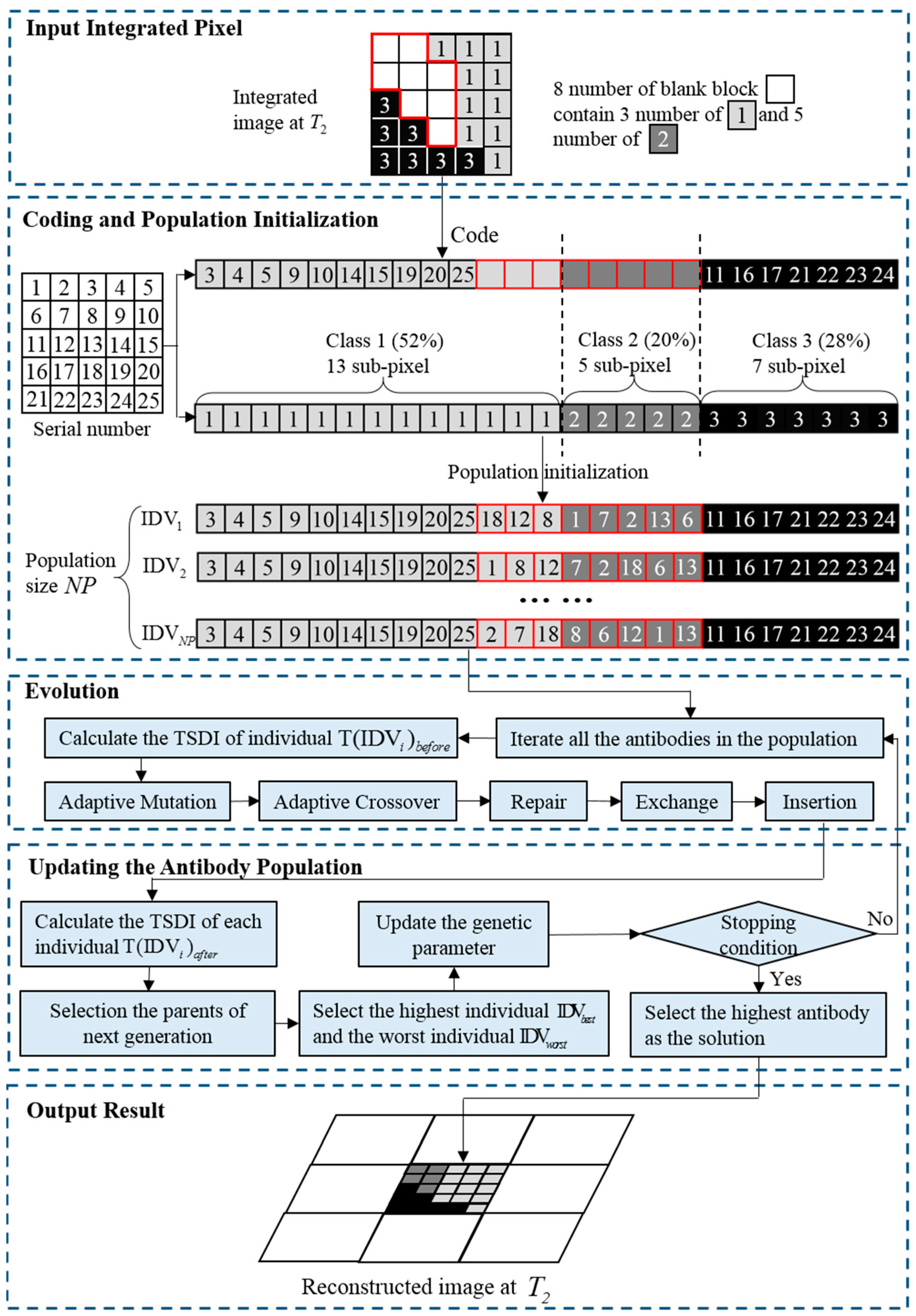
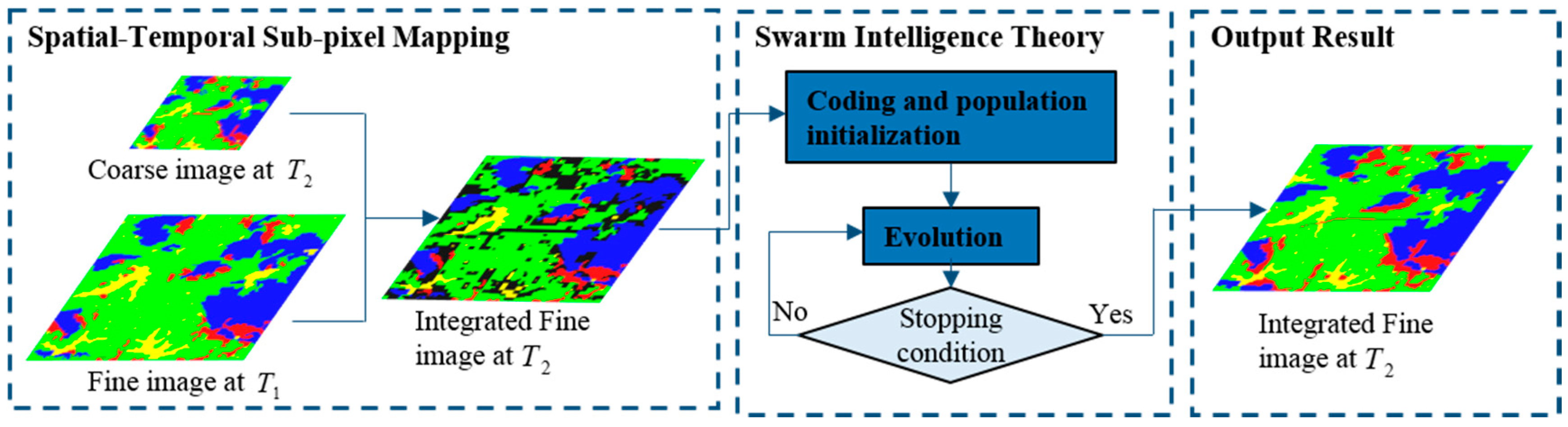
A number of studies have addressed incorporating the fine spatial resolution image into the sub-pixel mapping process. Nevertheless, these traditional algorithms and neural network algorithms, which search for the solution scholastically, are out of date. In this paper, we propose two spatial-temporal sub-pixel mapping algorithms based on swarm intelligence theory, to incorporate the distribution constraint from the fine spatial resolution image into the intelligent processes of the evolutionary algorithm, such as the classical events of coding, initialization of the population, crossover, mutation, etc. The framework of spatial-temporal sub-pixel mapping based on swarm intelligence theory is shown in
Figure 5. In order to reconstruct the spatial distribution of the coarse image at
, the fine image at
with the same FOV is borrowed by the spatial-temporal sub-pixel mapping to yield an integrated fine image at
. However, there are still many pixels that cannot be uniquely determined, which are represented by the black pixels in
Figure 5. Therefore, swarm intelligence theory is used to generate the optimal solution of the undetermined black pixels, outputting the final reconstructed fine image at
.
3.1. Spatial-Temporal Sub-Pixel Mapping
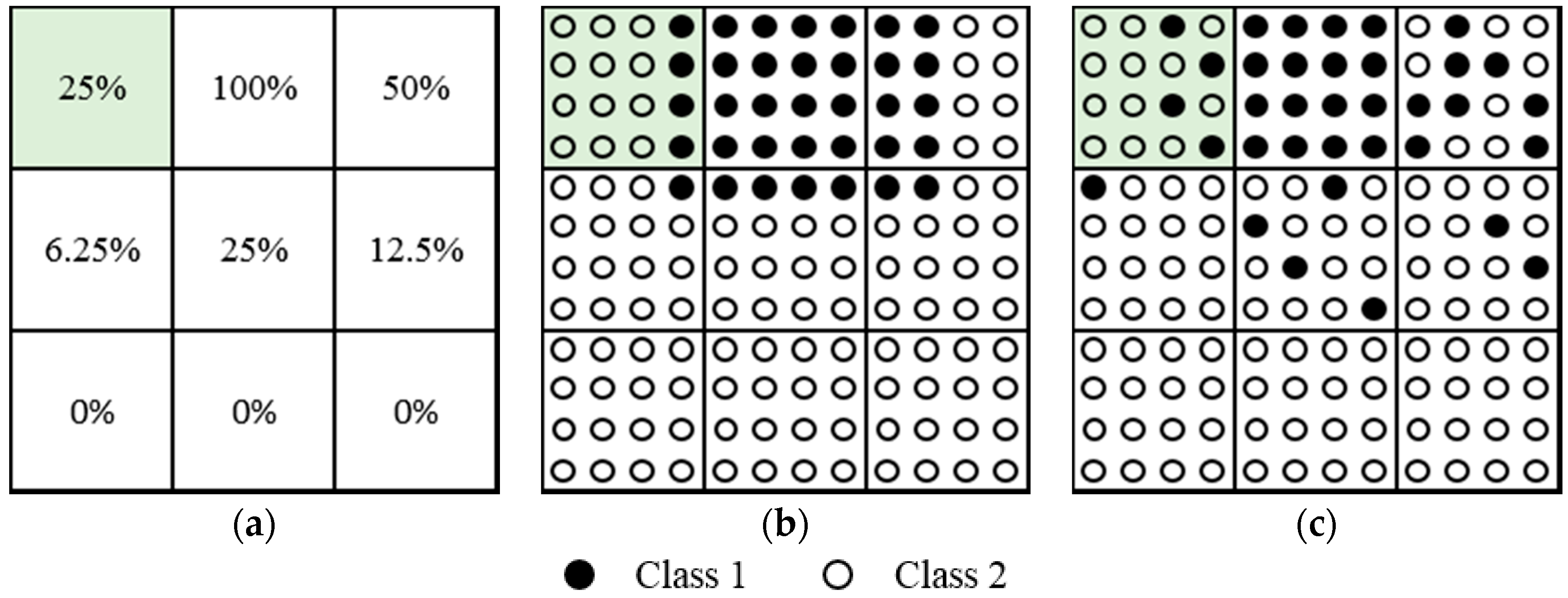
We suppose that the fine image at acquisition time
has been classified into three land-cover classes (light gray represents class 1, dark gray represents class 2, and black represents class 3), and spectral unmixing has been carried out on the coarse image (assuming that the spatial resolution of the fine image is five times that of the coarse image) at acquisition time
(assuming that time
and
are close) to obtain the abundance map for the three land-cover classes (52%, 20% and 28%) (one coarse pixel is shown in
Figure 6 as an example). A mean filter is then implemented to degrade the fine image (with the scale factor of five) at
to ensure that the proportion of the three land-cover classes (40%, 32% and 28%) is comparable to the unmixing result. During the time interval of
to
, it can be seen that class 1 has increased by 12%, which is equivalent to three (12% × 5 × 5) sub-pixels when transformed to the integer number of sub-pixels, and thus one can suppose that when one land-cover class has increased, some other land-cover class has changed to the increased class, but no increased class has changed to another class. Therefore, the unchanged part of the increased class can be copied to the distribution reconstruction of the coarse image, and the three extra sub-pixels of class 1 can only be allocated in the red circle. The upper situation in
Figure 6 is a possible distribution of class 1 in the coarse image at
. Meanwhile, class 2 has decreased by 12% during the time interval, and thus one may assume that when the land-cover class has decreased, no other class has changed to the decreased class, but the decreased class has changed to some other class. Therefore, the three sub-pixels of class 2 change to class 1, which is shown in the middle sub-figure, with the dotted area meaning that class 2 is about to change to class 1. For the black class, however, the proportion remains the same, and thus one can make the assumption that when the land-cover class remains unchanged, the spatial distribution of the class is also unchanged, which can be copied to the reconstruction of the coarse image.
Thus, both the fraction and real distribution of each class at the previous time are used, and the fraction is used as the determinant to decide whether or not each class increased or decreased, or was even unchanged, between the two temporal images. In addition, according to the fraction change tendency, we can decide which part of the real distribution at the previous time can be borrowed for the sub-pixel mapping of the imagery of the current time.
Integrating the land-cover map of the three classes, one can see that many sub-pixels can be uniquely determined for a certain class, except for the area within the red circle, which contains three sub-pixels of the light gray class and five sub-pixels of the dark gray class. In this paper, we use swarm intelligence theory as the optimization method to uniquely determine the position of the sub-pixels while maximizing the TSDI.
3.2. Swarm Intelligence Theory Based Spatial-Temporal Sub-Pixel Mapping
Swarm intelligence theory based sub-pixel mapping of a single-temporal image was introduced in the previous section. In this section, differing from the traditional GA, swarm intelligence theory is applied to a bitemporal image pair. To further improve the genetic process of swarm intelligence theory, two specific evolutionary algorithms are introduced in this section.
3.2.1. Spatial-Temporal Sub-Pixel Mapping Based on the Clonal Selection Algorithm (CSA)
The CSA is inspired by the human immune system, which can resist the infection of a virus by recognizing the extrinsic antigens. This algorithm generates a pool of candidate antibodies (solutions), selecting the most suitable antibodies corresponding to the antigens, and eliminates the antigens by the combination of the antigens and antibodies, thus solving the optimization problem [
55]. When detecting the assault of antigens, the immune system will generate a pool of candidate antibodies, and the antibody with the most affinity to the antigen will successfully combine with the antigen and eliminate it. Thus, the main mechanism of the immune system is the updating of the antibody pool to obtain the most suitable antibodies corresponding to the antigens. The updating mechanism consists of a series of maturation processes, such as cloning the antibodies with a higher fitness to pass on to the next generation for the reason of maintaining a suitable structure, replacing the antibodies with a lower fitness, and mutating to retain diversity of the antibody pool. Through this process of selecting superior antibodies to pass on and eliminating inferior antibodies generation by generation, the best antibody with the most suitable structure will be generated.
The CSA is derived from this mechanism and imitates the intelligent operations of cloning, selection, mutation, and elimination [
56]. The antigens are analogous to the coarse pixel to be reconstructed, and the antibody is the solution of the reconstruction map of that coarse pixel. The suitability degree of the antibody to the antigen is measured by the TSDI. In the CSA, the solutions with a higher TSDI are selected to reproduce clonal solutions as the next generation for the sake of maintaining good genetic information, and the solutions with a lower TSDI are eliminated to remove the bad genetic information from the population. In order to facilitate the maturation of the solutions while retaining the diversity of the solution pool, hypermutation is used, giving a chance for solutions to escape from local regions. More importantly, the operations of cloning and selection corroboratively confirm the convergence of the optimization problem [
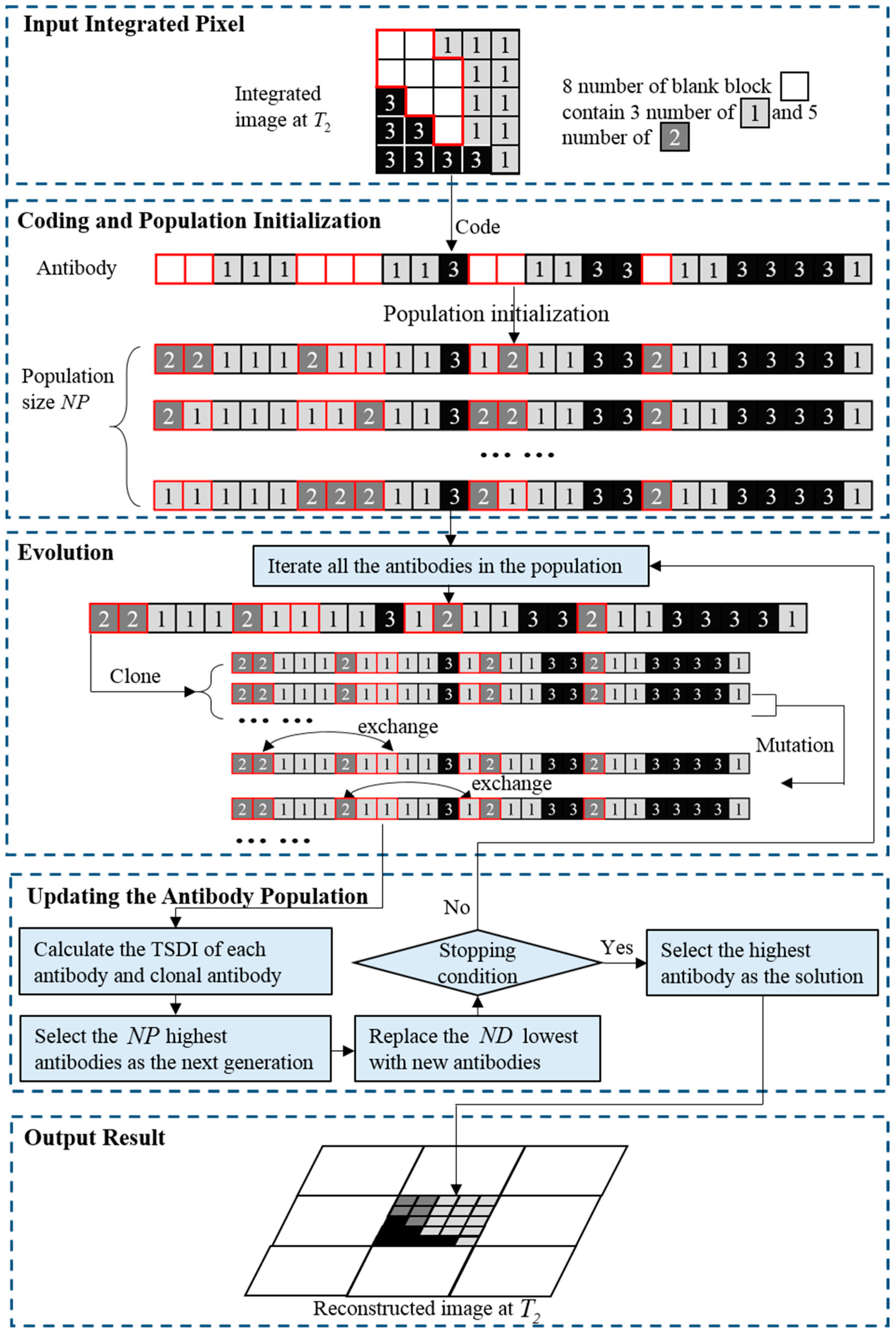
57]. The specific operation of the CSA can be described in the following steps.
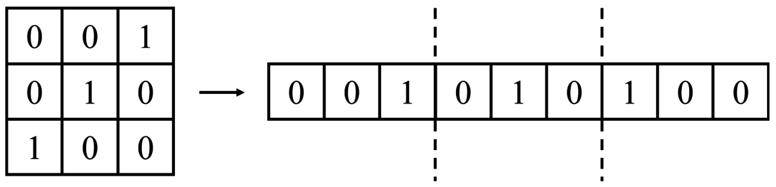
(1) Coding and population initialization
In the first step, the integrated land-cover map at
is first coded to the linear structure shown in
Figure 7 according to the clonal selection principle by connecting the first sub-pixel in each row to the last sub-pixel of the previous row, row by row. The operation of population initialization involves randomly assigning the three light gray classes and five dark gray classes to the empty position within the red circle, generating a certain number of antibodies according to the population size
. Each antibody
represents a possible spatial distribution pattern inside the coarse pixel. After initialization of the population, the TSDI of each antibody is calculated to obtain the highest TSDI value
and the lowest TSDI value
for further use.
(2) Evolution
After initialization of the population, the clonal operation is implemented to ensure that the better genetic information is passed on to the next generation. Each antibody
produces
clonal antibodies according to the formula:
where
is the clonal ratio parameter,
indicates the operation of confining the argument toward the nearest integer, and
represents the number of clones each antibody generates. After the process of cloning, each antibody has its clonal set
, and to ensure there is at least one antibody in the clonal set,
is set as no less than 1. Thus, the total number of antibodies in the population is equal to
.
The hypermutation operation is undertaken to avoid the solution falling into the local regions, while promoting the convergence of these intelligent processes to obtain the best solution with the highest TSDI. In this paper, in order to improve the intelligence of the evolutionary processes, we adopt an adaptive mutation operation, in which the mutation rate
is adaptively determined according to the fitness degree of the antibody
, as formulated below:
which is based on the principle that a higher fitness value deserves a lower mutation rate to avoid destroying the good structure of the antibodies in the population, while a lower fitness value deserves a higher mutation rate to remove the bad genetic information from the population, to better handle the hypermutation process. Parameter
is the decay factor defined by the user, and is usually set to 2. Because of the fraction constraint calculated before for determining the number of sub-pixels allocated to each land-cover class, it is unreasonable to simply change the attributes of any sub-pixel and subsequently break the constraint, and thus we take the measure of exchanging the attributes of the two randomly selected positions of the sub-pixel, achieving the effect of mutation.
(3) Updating the antibody population
After the hypermutation operation, the TSDI values of each antibody, as well as the mutated clones, are calculated to decide which antibodies can pass structural information on to the next generation, and the highest antibodies are selected as parents for the next generation. To retain diversity of the population and exploit the unknown solution space, the antibodies ranking at the end of the parents are replaced by newly produced antibodies. represents the number of displaced individuals, and was previously defined by the user. The stopping condition is set as a fixed number of generations, and the antibody with the maximum TSDI is selected as the optimal solution for the reconstruction of the coarse pixel and to output the result.
3.2.2. Spatial-Temporal Sub-Pixel Mapping Based on the Differential Evolution Algorithm (DEA)
The DEA is one of the latest global optimization methods, which searches for the solution heuristically in the global space [
58], and is incorporated into the framework of spatial-temporal sub-pixel mapping in this paper. A genetic operator such as crossover is adopted to take advantage of the differential information for facilitating the convergence of the solution, and the genetic parameters of mutation rate, crossover rate, and scale factor are adaptively determined by the adaptive scheme.
(1) Coding and population initialization
At the inception, differing from the coding mechanism in the CSA, the DEA codes the serial number of the sub-pixel instead of the class label, as shown in
Figure 8. The linear structure filled with only 1, 2, and 3 represents the class attribute position, which is constructed according to the fraction constraint of the coarse pixel at
. Therefore, the individual is generated by filling the attribute block with serial numbers according to the class block of the class attribute position. For example, in
Figure 8, the position with a serial number of 3 has the attribute number of 1, and thus the coding operation is implemented by filling the attribute block of class 1 with the serial number of 3, and the position with a serial number of 11 has the attribute number of 3, so the attribute block of class 3 is filled with the serial number of 11.
Each individual represents a possible spatial distribution pattern inside the coarse pixel, and the TSDI of each antibody is calculated for further use.
(2) Evolution
Differing from the traditional mutation operation of simply exchanging the attributes of two sub-pixel positions, the individual undergoing the mutation is regenerated by adding the weighted difference of two randomly selected individuals to a third randomly selected one, which is formulated as follows:
where the indices of
and
are randomly generated within the range [1, NP] and are mutually exclusive, as well as
, which means
.
is a scale factor parameter of the
individual in the
generation, which can balance the scale of the difference.
represents the
individual of the
generation, and
indicates the newly generated
individual of the
generation as an intermediate quantity.
The crossover operator is then implemented and can be defined as follows:
where
represents the serial number of the
position in the
individual of the
generation, and
represents the corresponding serial number after the mutation operation.
is a randomly generated number ranging from 0 to 1.
is the genetic parameter of the crossover rate, which determines the probability of the crossover operation.
In order to determine the genetic parameters adaptively, instead of manually, which is time-consuming, an adaptive strategy is adopted based on the principle that the better individuals are more likely to survive and pass on better genetic information (better structural information) to the next generation, and is formulated as follows:
where
and
represent the crossover rate and scale factor of the current generation, while
and
indicate the genetic parameters of the next generation, respectively.
,
, and
are randomly generated numbers within the range [0, 1]. IG represents the total number of generations of the differential evolution process defined by the user.
is the nonconforming degree parameter, and is empirically set to 3 [
59].
is the mutation rate, which acts as a threshold of the adaptive scheme, depending on the best and worst TSDI values of the current generation, and is formulated as follows:
where
means the TSDI value of the
individual in the
generation, and
and
represent the best and the worst TSDI values of the
generation, respectively.
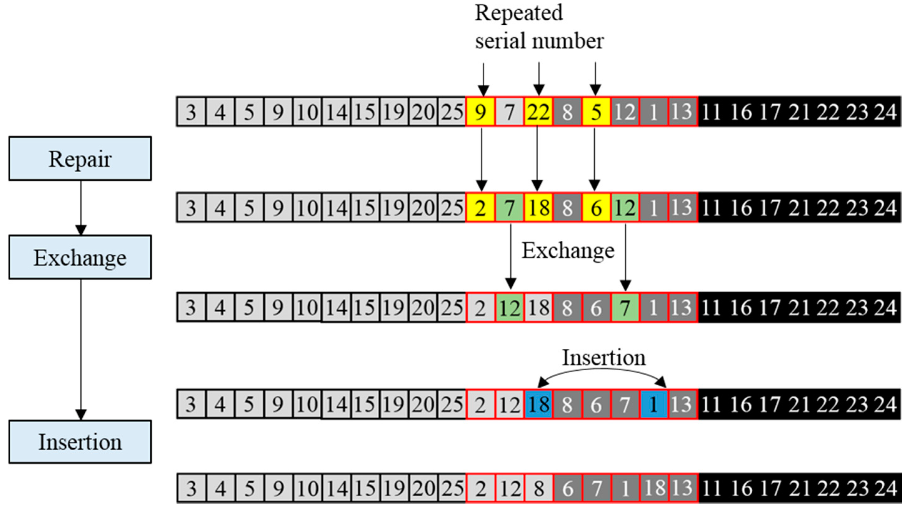
After the adaptive mutation and crossover operations, more intelligent processes need to be implemented to further improve the individual. Considering that repeated serial numbers inside the individual might emerge due to the process of mutation, further measures should be taken to repair the repeated positions, and the process is shown in
Figure 9. Serial numbers 2, 6, and 18 are missing, and 9, 22, and 5 are repeated, and thus should be replaced to repair the integer of the serial number of the individual. The exchange operator is then implemented to improve the individual by randomly selecting two positions and exchanging the serial numbers inside the positions. Finally, an insertion operation is undertaken to stochastically disturb the solution and facilitate the convergence by randomly selecting two positions, putting the front serial number to the position behind the next serial number, as shown in
Figure 6.
(3) Updating the population
After the process of evolution, the TSDI of each antibody is calculated to decide the parents of the next generation, as follows:
where
and
represent the
individual in the
generation before and after the process of evolution, respectively. Only if the TSDI of the
individual improves during the process of evolution can this individual pass the structural information on to the next generation. The best TSDI and the worst TSDI in the current generation are then calculated for the updating of the mutation rate, crossover rate, and scale factor.
The stopping condition in the differential evolution also adopts a fixed number of generations, and the individual with the maximum TSDI is selected as the optimal solution for the reconstruction of the coarse pixel, and to output the result.
Although the two proposed algorithms have similar main frameworks, both of which are based on natural selection and the natural genetic principle, searching for the most plausible solution in the global population stochastically but heuristically by emulating the biological advantage of the human system, they are different in the coding method and evolution process. Both algorithms are implemented with several evolution operators on a set of solutions (population) and an adopted adaptive strategy to determine the genetic parameters, and each solution is scored by a fitness value calculated based on the spatial dependence. The solution with the highest score is then selected to be the parent of the next generation. However, the coding method of SSMCS is based on the class attributes, and it simply transforms the square structure to a linear structure by connecting the first sub-pixel in each row to the last sub-pixel of the previous row. Meanwhile, the coding method of SSMDE is based on the serial number of each sub-pixel in the individual, and the linear structure is divided into several class attribute blocks according to the fraction constraint. We then fill these blocks with the serial numbers of each sub-pixel according to their class attributes. Furthermore, the evolution processes of SSMCS and SSMDE are also different. SSMCS evolves the solution population by a cloning operator and a mutation operator. On the other hand, SSMDE evolves the solution population by an advanced mutation operator which adds each individual to the differential of another two individuals, as well as the crossover operator, which is not included in SSMCS.
4. Experiments and Analysis
We designed three experiments to demonstrate the effectiveness of the proposed algorithms (SSMDE, SSMCS) visually and quantitatively, and a number of previous sub-pixel mapping algorithms were used to make a comparison: pixel swapping sub-pixel mapping (PSSM) [
11], sub-pixel mapping based on a genetic algorithm (GASM) [
49], sub-pixel mapping based on clonal selection (CSSM) [
56], sub-pixel mapping based on differential evolution (DESM) [
58], as well as the spatial-temporal sub-pixel mapping versions of these algorithms (spatial-temporal sub-pixel mapping based on a pixel swapping algorithm (SSMPS) [
35], spatial-temporal sub-pixel mapping based on a genetic algorithm (SSMGA) (spatial-temporal sub-pixel mapping based on a genetic algorithm (SSMGA) has not been proposed so far, and we just added the spatial-temporal sub-pixel mapping principle to GASM to generate SSMGA), to examine the validation of the spatial-temporal sub-pixel mapping principle. The population size, crossover rate, and mutation rate in GASM and SSMGA were set to 100, 0.5, and 0.5, respectively. In CSSM and DESM, the crossover rate and mutation rate employ an adaptive strategy during the generation, so we just needed to determine the population size, which was set to 100 (the clonal rate
was set to 0.02 and
was set to 10 in CSSM). The overall accuracy (OA) and Kappa coefficient were calculated for the quantitative assessment of the accuracy of the proposed sub-pixel mapping algorithm. Furthermore, since the experimental datasets were bitemporal image pairs, LCCD was conducted between the sub-pixel mapping result and the fine spatial resolution image during each experiment (the LCCD was simply implemented by differentiating the sub-pixel mapping result with the fine spatial resolution image and then classifying the differential map into two classes: changed areas and unchanged areas). OA and Kappa consider all the pixels of the image, including the pure pixels, as parents in the finer resolution. These sub-pixels all belong to the pure pixels and will only raise the value of OA and Kappa, without providing information about the algorithm’s predictive abilities. To improve the reliability, adjusted OA (OA*) and adjusted Kappa coefficient (Kappa*) were developed, which only take the mixed pixels into consideration and ignore the pure pixels, because the sub-pixel mapping method only reconstructs the mixed pixels, and the pure pixels would consequently increase the OA and Kappa, masking the true contribution of the tested algorithm. These criteria have been proved to be useful in the published paper by Mertens et al. [
41].
4.1. Experiment 1: Landsat 8 Image
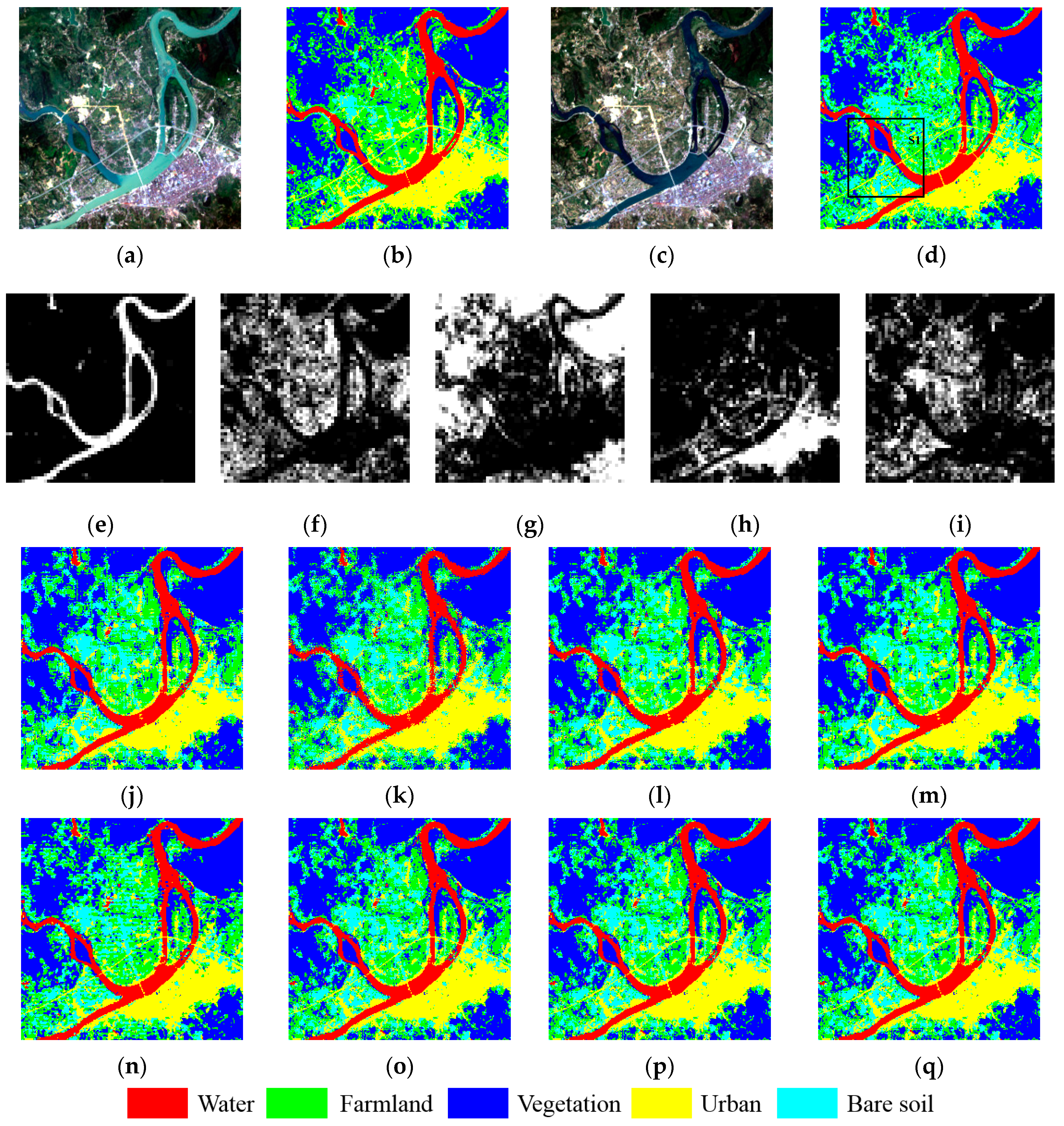
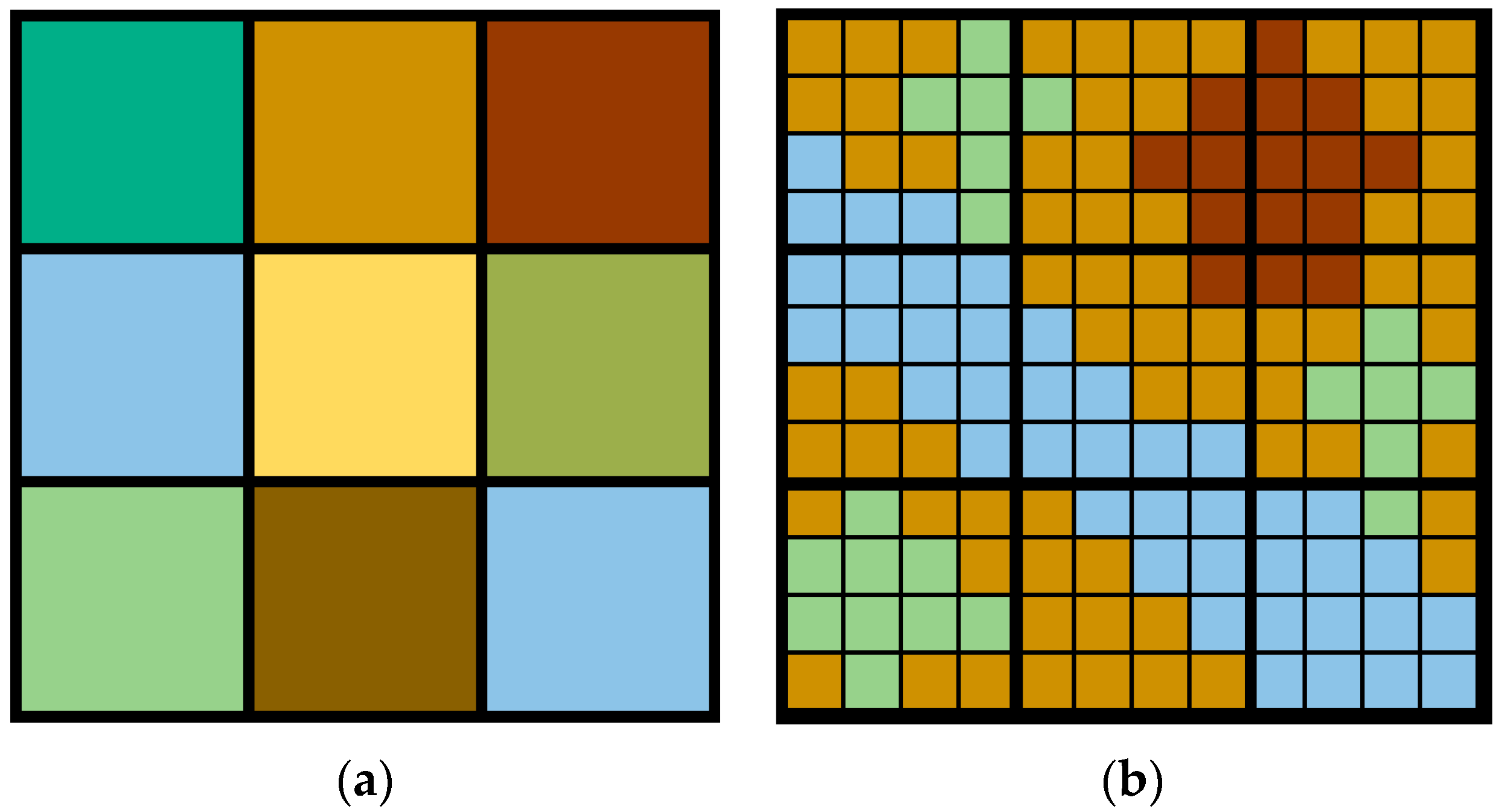
In Experiment 1, we obtained bitemporal Landsat 8 images from Cili County, Hunan province, in which the farmland areas are abundant, as shown in
Figure 10a,c. The acquisition times of the bitemporal images were 13 July 2013, and 7 August 2013, respectively. The time interval is 25 days, and it is worth noting that 7 August is the beginning of the autumn in the 24 solar terms in China, by which time many farmland crops are ripe and being harvested, and thus more bare soil would appear compared to the image of 13 July. Together, these images exactly meet the condition of frequent change over a small time interval. We split the test area into subsets of 240 × 240, with a resolution of 30 m. The coordinates of the selected test area are (29°4′45.66″–29°8′38.60″N) and (111°0′19.21″–111°4′45.27″E), with the north arrow toward the upside. A supervised hard classification method—support vector machine (SVM)—was applied to the bitemporal Landsat 8 images to generate the land-cover maps (
Figure 10b,d) to be used for the degrading and accuracy assessment. The land-cover maps were classified into five land-cover classes: water, farmland, vegetation, urban, and bare soil.
Synthetic images were used as the input fraction images, and were obtained by degrading the hard classification image from 7 August to a coarser scale using an averaging filter of four. We chose synthetic imagery to verify the validation of the proposed algorithm so as to avoid coregistration errors between the lower- and higher-resolution images, the sensor point spread function, the atmospheric effect, and the spectral unmixing error, and thus the sub-pixel mapping results solely illustrate the performance of the different algorithms.
Figure 10e–i shows the degraded fraction image, and the sub-pixel mapping results of PSSM, GASM, DESM, CSSM, SSMPS, SSMGA, SSMDE, and SSMCS are displayed in
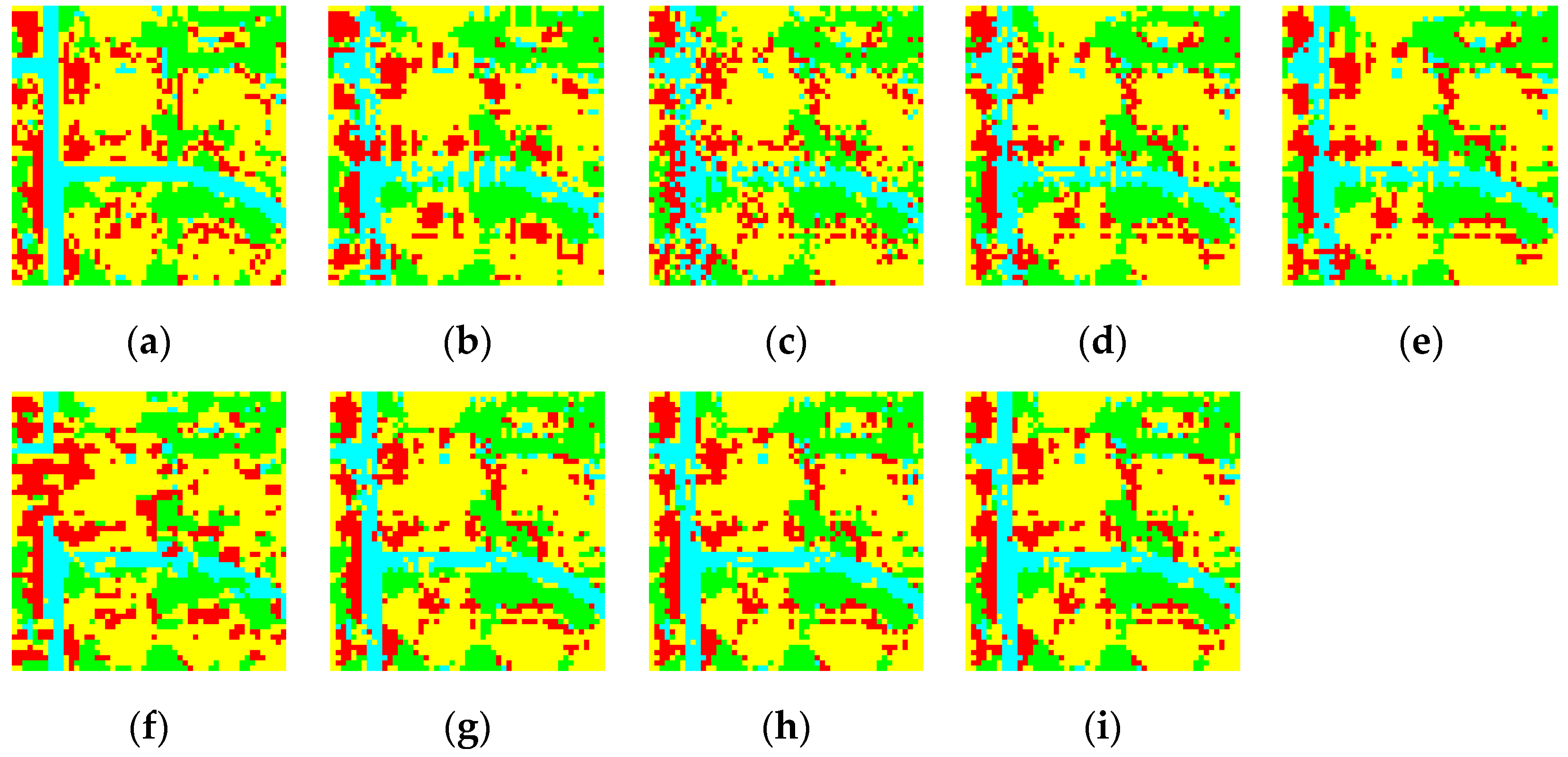
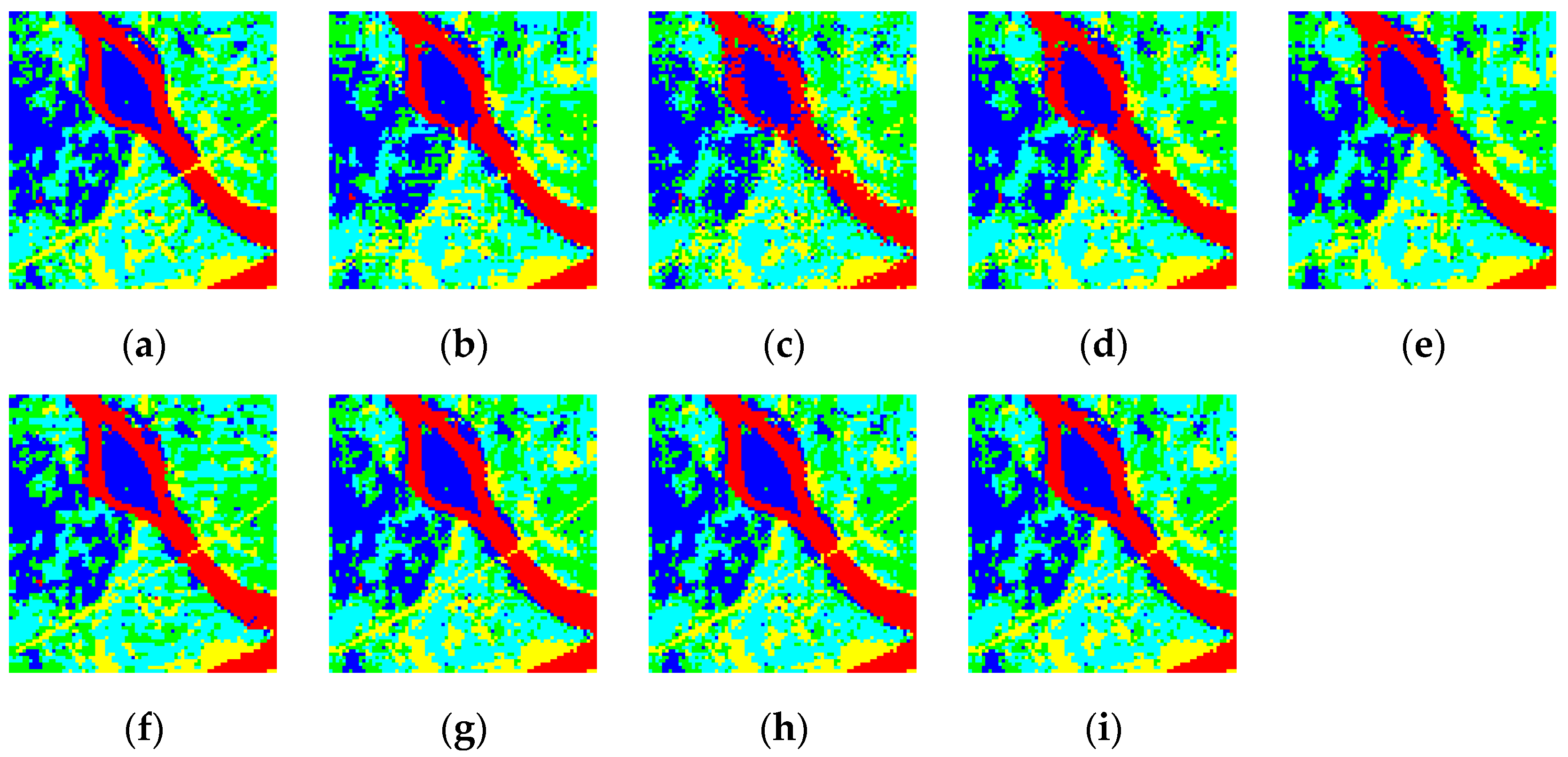
Figure 10j–q. To further examine the performance of the reconstruction of detailed land cover, the small area of S1 is zoomed in on in
Figure 11a–i.
According to the visual assessment, as can be clearly seen in the zoomed version in
Figure 11, GASM is weak at preserving boundary features such as the coastline. Linear features, such as bridges and roads, are almost entirely missing in the results of the traditional methods. When compared with the other algorithms, SSMGA, SSMDE, and SSMCS outperform the other methods, giving a better linear reconstruction and smoother boundaries, and are more consistent with the reference. As for the quantitative evaluation in
Table 1, the OA and Kappa values of the SSMDE and SSMCS are almostly the same, and are the best among all the algorithms, reaching 81.62%, 0.7584 and 81.61%, 0.7584, respectively, while the accuracies of SSMGA are slightly lower than SSMDE and SSMCS. The advantage of the proposed algorithms are also shown for LCCD in
Table 2, in which the SSMDE and SSMCS algorithm obtains a higher OA of 84.15% and 84.13%, respectively. To solely examine the reconstruction of the mixed pixels and ignore the influence of the pure pixels, the OA* and Kappa* were also calculated, where SSMDE and SSMCS again obtain the best result. The reason for this is down to the advantage of the genetic operators such as crossover, mutation, and selection, which can exchange information adequately to obtain the optimal solution, and the advantage of the spatial-temporal sub-pixel mapping principle, which can incorporate the distribution information of the fine spatial resolution image to regularize the ill-posed sub-pixel mapping problem.
In this way, the synthetic coarse image of 7 August 2013 can be seen as the daily obtained MODIS image, with frequent temporal information but coarse spatial resolution. Meanwhile, the original Landsat 8 image of 13 July 2013 can provide the high spatial resolution, but the 16-day revisit period missed the growth cycle at the beginning of autumn. Therefore, the proposed algorithm can fuse the temporal information of MODIS and the spatial information of Landsat to obtain a high-resolution image at the missing growth cycle time. The experimental results confirm that the proposed algorithm outperforms the traditional approaches, achieving a better sub-pixel mapping result, both qualitatively and quantitatively. Furthermore, it also achieves a change map with both a fine spatial resolution and a fine temporal resolution, exactly meeting the demands of timely and detailed LCCD.
4.2. Experiment 2: QuickBird Image
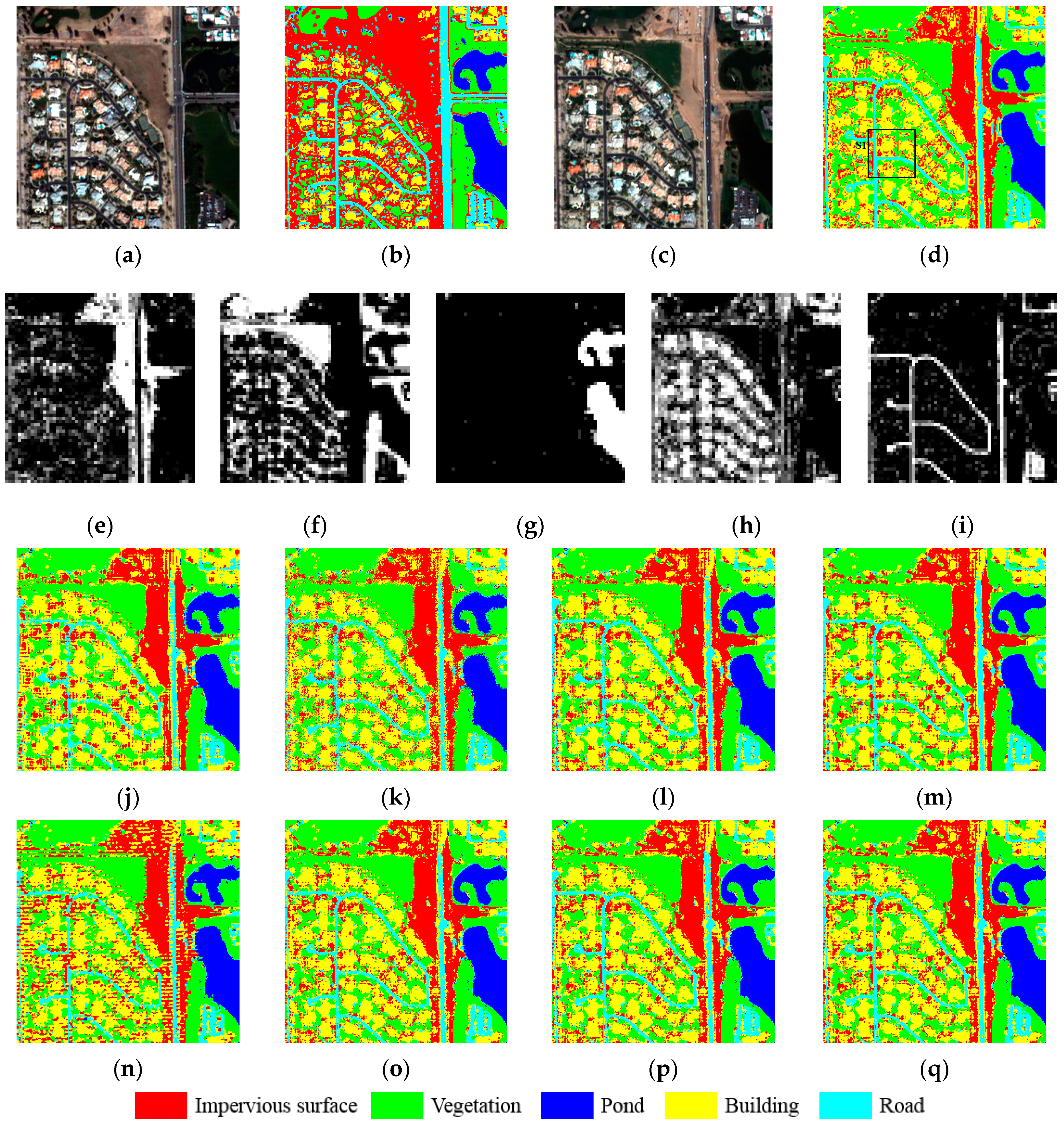
In Experiment 2, bitemporal QuickBird images of 240 × 240 (at a 2.5-m spatial resolution) of the urban area located at Shiyan City, Hubei province, which were acquired in 2002 (
Figure 12a) and 2004 (
Figure 12c), respectively, were taken into consideration to further examine the performance of the proposed algorithm. The coordinates of the QuickBird images are (413,616.00–414,211.20 m E) and (3712,485.60–3713,080.80 m N), with the north arrow toward the upside. A supervised hard classification method—support vector machine (SVM)—was applied to the bitemporal QuickBird images to generate the land-cover maps (
Figure 12b,d) to be used for the degrading and accuracy assessment. The land-cover maps were classified into five land-cover classes: impervious surface, vegetation, pond, building, and road. Experiment 2 also adopted a synthetic strategy, as in Experiment 1, to avoid the errors introduced by coregistration and spectral unmixing. The SVM hard classification of the QuickBird image from 2004 was degraded by a mean filter with a scale factor of four to yield the fraction maps shown in
Figure 12e–i.
Figure 12j–q shows the sub-pixel mapping results of PSSM, GASM, CSSM, DESM, SSMPS, SSMGA, SSMDE, and SSMCS, respectively, and the zoomed area of S1 showing the detailed reconstruction of each algorithm is shown in
Figure 13a–i.
According to the visual assessment, when compared with
Figure 13a, one can see that CSSM is better able to reconstruct the scattered impervious surfaces (shown in red) than PSSM, which reconstructs the discrete scattered land cover into a continuous blocky area, thus losing much of the detailed information. Meanwhile, the results of GASM and DESM are less pleasing due to the discontinuous land-cover boundaries and noise. The performance of the reconstruction of the linear road (shown in blue) is disappointing in all the sub-pixel mapping algorithms, except for SSMCS, as shown in
Figure 13, where it effectively reconstructs the linear road, as well as the other land covers, and the distribution pattern is the most similar to
Figure 13a. On the other hand, in
Table 3, the quantitative accuracy result is consistent with the visual assessment, where for the OA, SSMCS achieves the best result of 80.98%, and the performance of SSMDE resembles SSMGA. In
Table 4, the SSMDE and SSMCS also outperform the others in terms of LCCD with higher OA of 88.08% and 88.20%, respectively. A possible reason for this can be ascribed to the transformation of the sub-pixel mapping problem into the swarm intelligence based optimization problem, enabling us to search for a solution in a continuous solution space, thereby guaranteeing the continuity of the land cover and yielding a smoother result. The strategy of the spatial-temporal model also contributes to the more accurate result, due to the detailed spatial information it obtains from the fine spatial resolution image to regularize the under-determined sub-pixel mapping problem.
4.3. Experiment 3: Real Image
Although the synthetic images utilized in Experiments 1 and 2 can avoid the errors introduced by coregistration or spectral unmixing, allowing us to solely evaluate the performance of each sub-pixel mapping algorithm, this does not meet the practical requirement of applying the algorithm directly to a real low spatial resolution image, instead of a synthetic image generated by degrading the hard classification image. Therefore, sub-pixel mapping of a real low spatial resolution image (MODIS) was implemented in Experiment 3, and a Landsat TM image with almost the same acquisition area was chosen to evaluate the performance of each algorithm. Given that coregistration and spectral unmixing are considered as preprocessings of each sub-pixel mapping algorithm, the performances of each sub-pixel mapping algorithm could be considered to be comparable due to the same errors being introduced by these preprocessing operations. It is worth noting that the synthetic process can avoid the coregistration errors between the lower- and higher-resolution images, the sensor point spread function, the atmospheric effect, and the spectral unmixing error, and the sub-pixel mapping results solely illustrate the performance of the different algorithms; on the other hand, the real experiment process considers the practical requirement of applying the algorithm directly to a real low spatial resolution image, and can test the adaptability and expansibility of the proposed algorithm. Both the synthetic and real processes are feasible, and they just focus on different aspects and work for different purposes.
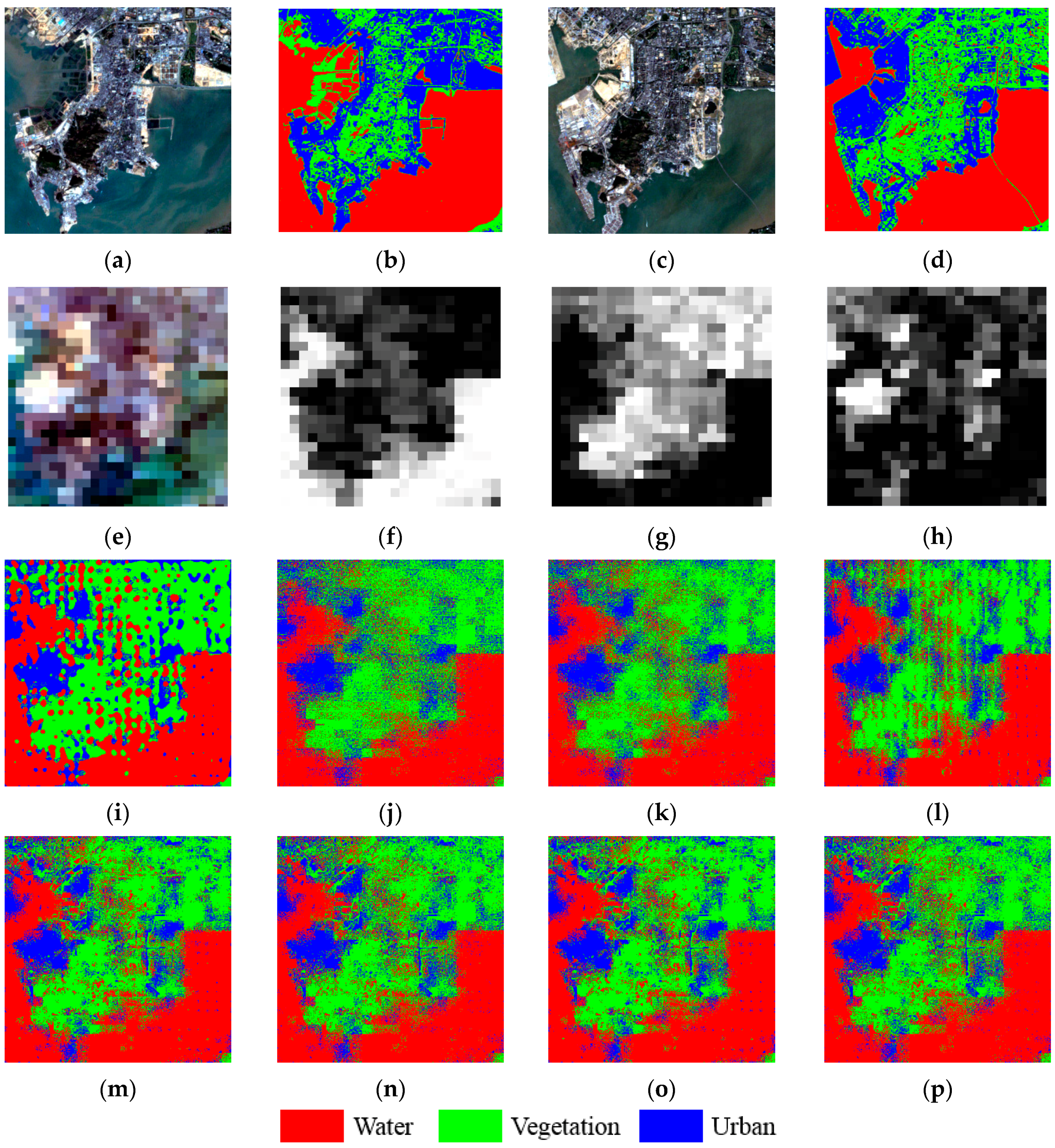
The MODIS surface reflectance product (24 × 24) acquired at Shenzhen City, Guangdong province, on 12 October 2009, with a spatial resolution of 500 m, was chosen as the low spatial resolution image to be reconstructed, which is shown in
Figure 14e, and the Landsat TM image (408 × 408) acquired in the same area with a 30-m spatial resolution on 12 August 2001, as shown in
Figure 14a, was selected as the fine spatial resolution image to provide a distribution pattern for the reconstruction process. The Landsat Enhanced Thematic Mapper (ETM) image acquired on October, 2009, at the same scene, was used to obtain a fine spatial resolution classification result as the reference to evaluate the accuracy of each algorithm by the k-means method, as shown in
Figure 14c,d, respectively. The coordinates of the Landsat ETM+ image and MODIS image are (113°1′25.85″–113°8′32.45″E) and (22°7′21.00″–22°3′42.20″N), and the north arrow is toward the upside.
Three steps were taken to complete the preprocessing. Firstly, the TM image from 2001 was classified into three land-cover types (water, vegetation, and urban) using the k-means method, as shown in
Figure 14b. The coregistration process was then implemented between the MODIS image from 2009 and the TM image from 2001, so that each fine pixel in the TM image had a corresponding coarse pixel in the MODIS image, using the ground control point function provided in ENVI software. During the coregistration, the MODIS image was resampled to 510 m to match the TM image (30 m) data by 17 times. Finally, fully constrained least squares (FCLS) linear spectral unmixing was carried out to generate fraction images of the MODIS image, as shown in
Figure 14f–h. After the preprocessing, we could use the standard data to implement the sub-pixel mapping algorithms, and the results are displayed in
Figure 14i–p. As for the quantitative accuracy assessment, we used the classification result of the 2009 TM image (
Figure 14d) to compare with the sub-pixel mapping result to obtain the statistics shown in
Table 5. In order to evaluate the performance of the LCCD generated by each sub-pixel mapping method, we overlaid the classification result of the 2001 TM image on the classification result of the 2009 TM image to produce a differential map as the reference LCCD result, and each sub-pixel mapping result was overlaid on the classification result of the 2001 TM image to generate the LCCD result, which was then compared to the reference LCCD result to obtain the statistics of the LCCD accuracy, as shown in
Table 6.
In the visual assessment, one can see that PSSM loses almost all the structural information and boundary information between the different classes, showing a fuzzy classification for the whole map. Although the result of GASM contains some structural information when compared to PSSM, there is a lot of noise, which compromises the visual effect to a great extent. On the other hand, the results of DESM and CSSM are better than the results of PSSM, providing relatively clear boundaries between classes, but the inner structure of each class is still fuzzy. All the sub-pixel mapping results are more or less fuzzy and disappointing, except for the spatial-temporal fusion based sub-pixel mapping methods (SSMPS, SSMGA, SSMDE, and SSMCS), which better reconstruct the structural information between and within classes, and are less affected by noise, when compared to the results of the aforementioned traditional methods. Although the results (SSMPS, SSMGA, SSMDE, and SSMCS) appear similar, the quantitative assessment can be used to further distinguish the algorithms.
When it comes to the quantitative assessment, we can see in
Table 5 that the accuracies of all the sub-pixel mapping algorithms are lower than those in the synthetic experiments, which may be due to the errors induced by the coregistration and spectral unmixing operation and the classification errors of the TM image. The scale factor
is another reason for the compromised statistical accuracy, where, according to the principle of the sub-pixel mapping problem, one coarse pixel should be reconstructed to an
fine pixel, which indicates that a larger scale factor means a more complex reconstructed scene, thereby generating a lower accuracy. Nevertheless, SSMCS still acquires a reasonable accuracy when compared to the other algorithms with regard to OA and Kappa, reaching 64.50% and 0.4533, respectively. Meanwhile, SSMDE and SSMGA obtain a relatively high OA of 64.18% and 64.24%, respectively. Note that all the adjusted OA and Kappa values are the same as the normal OA and Kappa values in Experiment 3, since the adjusted OA and Kappa only take the mixed pixels into consideration, and, in this case, the spatial resolution of the MODIS image is 500 m, which is large enough that one pixel could contain several land-cover types. During the spectral unmixing process, all the pixels were determined as mixed pixels. Therefore, the adjusted OA and Kappa values are all the same as the normal OA and Kappa values. As for the subsequent LCCD results in
Table 6, the results are consistent with the sub-pixel mapping results, and SSMCS obtains the best LCCD accuracy of 70.93%, confirming the superiority of the proposed algorithm, regardless of the low accuracy.
The main limitation of this technique is the full constraint of the fractions derived from the spectral unmixing technique. As we know, the abundance map generated by the spectral unmixing process is the input of the sub-pixel mapping method; however, the error of the spectral unmixing is introduced into the following sub-pixel mapping process and seriously compromises the sub-pixel mapping result. This is why the proposed method in real Experiment 3 has a limited advantage, while, in synthetic Experiments 1 and 2, which use the degraded image as input, it has a noticeable advantage over the other algorithms.
4.4. Computational Complexity
We can consider the computation time in terms of computational complexity, which can reflect the computation time from a macro perspective. Furthermore, the computational complexity is more convincing since the computation time is related to many uncertainties, such as the actual coding strategy in the program, the programing platform, the configuration of the user’s PC, etc.
The complexity of SSMCS can be split into four parts: (1) the integration of the previous high-resolution image; (2) the step of population initialization and coding; (3) the step of cloning and mutation according to the clonal rate and mutation rate pm; and (4) the step of TSDI calculation and population updating. We assume that the number of land-cover classes is C, the total number of pixels in each dimension of the input abundance map is M × N, the scale factor of the sub-pixel mapping is s, the population size is NP, and the generation number is G. Since only one coarse pixel is processed at a time, the computational complexity should be multiplied by M × N, so the computational complexity of part 1 is O (M × N × C), which is independent of the following part. For part 2, the complexity is O (M × N × s2), since the initialization and coding involve a sub-pixel scale. In part 3, the computational complexity is O (M × N × s2 × × NP × G) due to the mutation processing for every antibody in every generation, and the clonal processing only functions on the total number of antibodies. As the parts of initialization, coding, cloning, and TSDI calculation are dependent parts, they have the total computational complexity of O (M × N × s2 × × NP × G). Considering all the aforementioned parts, the total computational complexity of SSMCS is O (M × N × C + M × N × s2 × NP × G).
The complexity of SSMDE can also be split into the same parts as SSMCS, except for part 3, which contains the mutation operator and crossover operator. The total computational complexity of the generation part is therefore O (M × N × s2 × 2 × NP × G). Taking all four parts into consideration, the total computational complexity of SSMDE is O (M × N × C + M × N × s2 × 2 × NP × G).
5. Sensitivity Analysis
The proposed algorithms have several important parameters, including the scale factor s determining the complexity of the reconstructed scene, and the genetic parameters controlling the genetic process of evolution, which have a significant impact on the result of the reconstructed map. Since the sub-pixel mapping results were only analyzed at the scale factor of 4 in the synthetic experiments, multiple scale factors were also tested on the synthetic images used in Experiments 1 and 2 to examine the performance of the proposed algorithm.
The main genetic parameters are as follows:
- (1)
is the mutation rate parameter in SSMCS.
- (2)
is the crossover rate parameter in SSMDE.
Beside, the genetic parameters are adaptively determined by the adaptive strategy proposed in this paper, the two synthetic images used in Experiments 1 and 2 were again chosen to verify the adaptive strategy, and the results obtained by the adaptive parameters were compared with the non-adaptive results of different values of the genetic parameters.
5.1. Sensitivity in Relation to the Scale Factor
To explore the sensitivity of the proposed algorithm in relation to scale factor s, all the other parameters were kept the same as in Experiments 1 and 2. The scale factor was then set as s = {4, 5, 10}, and the corresponding OA accuracy of different algorithms were serve as the benchmark.
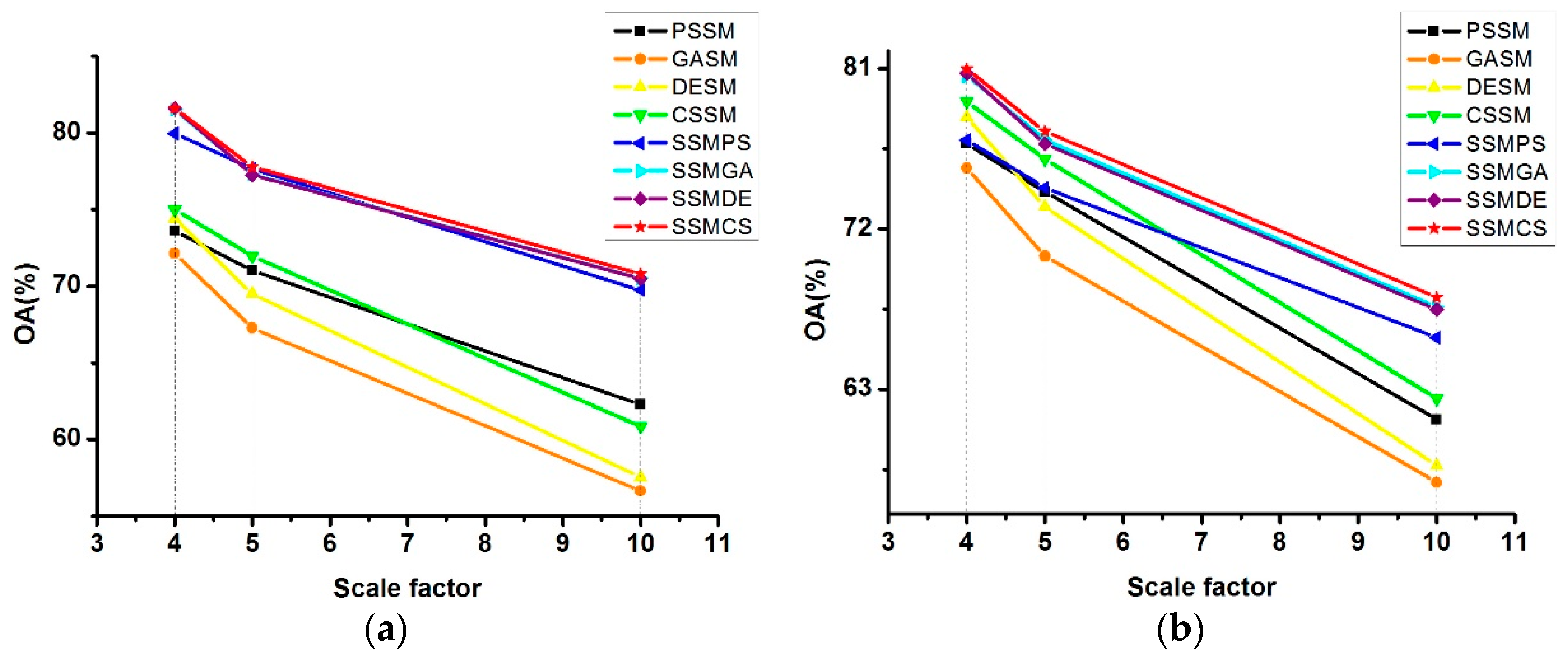
As shown in
Figure 15, the OA values are negatively correlated with the scale factor, i.e. the higher the value of scale factor
s, the lower the OA value. This is because the distribution of the land-cover classes becomes more complex as the scale factor
s increases, leading to an increase in the difficulty of the sub-pixel mapping. Given the fact that the accuracy of the synthetic images decreases as the scale factor increases, the proposed algorithms are still superior to the others. From the line chart, one can see that SSMDE and SSMCS are relatively stable with the increase of the scale factor, as the slope is gentler. What is more, SSMDE obtains the highest OA when the scale factor equals 4, and SSMCS performs the best at the scale factors of 5 and 10 in Experiment 1. As for Experiment 2, SSMCS performs better than the other methods at all the scale factors.
5.2. Sensitivity in Relation to the Mutation Rate Parameter in SSMCS
In SSMCS, the mutation rate parameter plays an important role in the evolution process of the generation. It controls the balance of the convergence of the solution and the preservation of the suitable structural information of the antibodies. If the mutation rate is too low, there is not enough disturbance to escape from the local optima. On the other hand, the suitable structural information will be destroyed if the mutation rate is too high. Therefore, the value of has a significant impact on the accuracy of the output result. In this paper, we develop an adaptive strategy to automatically find the most suitable value, which is based on the principle that a better individual deserves a lower mutation rate to avoid destroying the good structure, whereas a worse individual deserves a higher mutation rate to remove the bad genetic information from the population, and thus the value adaptively changes in every generation. In order to verify the effect of the adaptive strategy, several non-adaptive parameters were selected within the range [0.1, 1] with the same footstep of 0.1, to obtain the best non-adaptive parameter setting, which was then compared to the best adaptive parameter setting. It is worth noting that the selected value of the non-adaptive parameter did not change during the iteration process.
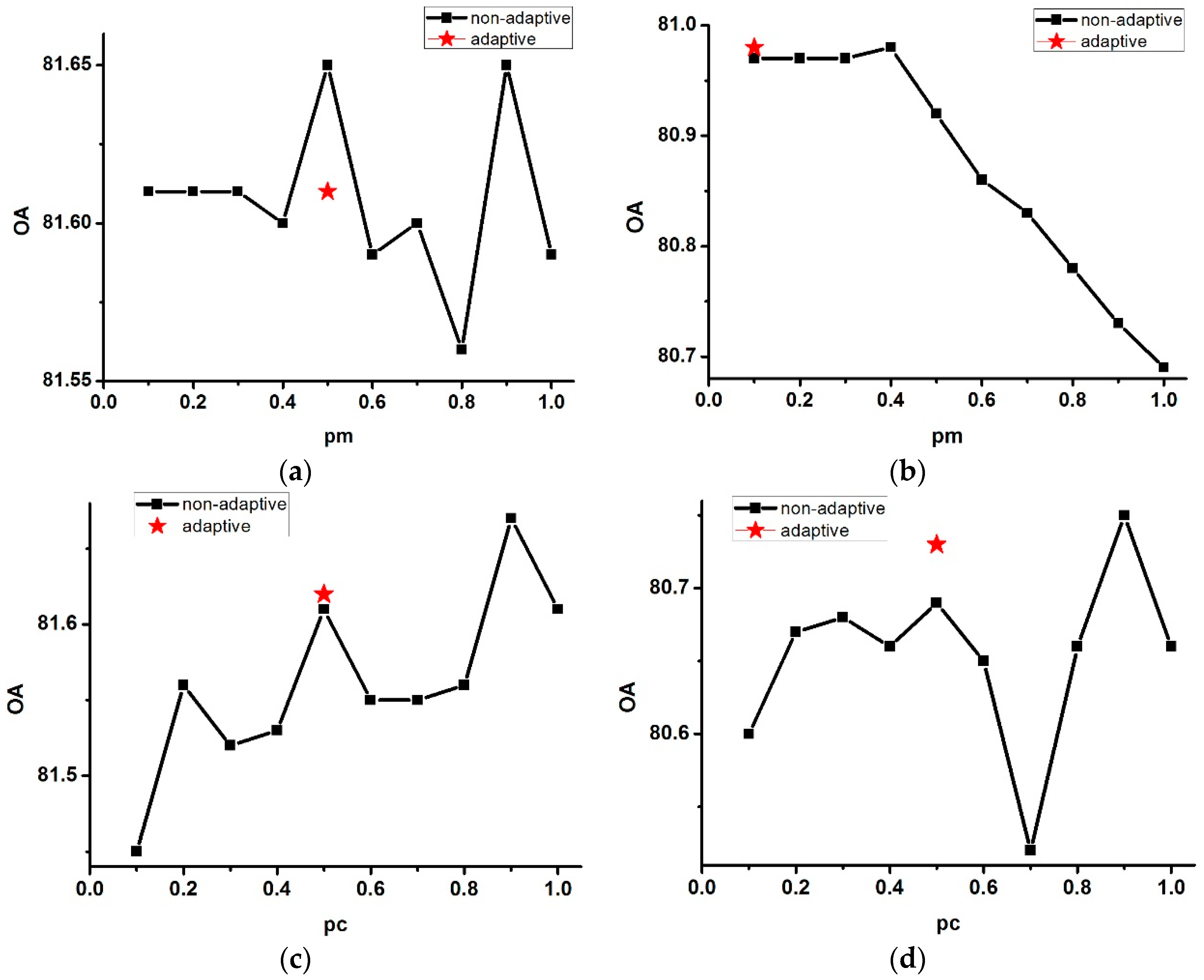
Figure 16a,b shows the OA curves of the results generated by the series of non-adaptive parameter
values for the synthetic images of Experiments 1 and 2, respectively. Since the adaptive values were updated in the iteration, we only show the final estimated adaptive values, as well as the OA values, which are represented by the stars. As displayed in
Figure 16a,b, the OAs of the results obtained by the adaptively estimated parameters are almost the same with the best OAs obtained by the non-adaptive parameters. As the values of the adaptively estimated parameter
are close to the best non-adaptive ones, this confirms the feasibility of the adaptive strategy. It is worth noting that since the
values are randomly initialized in the adaptive strategy, the
value will finally converge around the best
value manually selected, which corresponds to better OA values. Therefore, the adaptive strategy can be considered to be stable and robust, and moreover, release the time consuming manual work.
5.3. Sensitivity in Relation to the Crossover Rate Parameter in SSMDE
The crossover rate is one of the most important parameters in the operation of SSMDE. The crossover rate controls the rate of the exchange of differential information between an individual of the current generation and the next generation. Since a larger parameter value means an inclination to exchange superfluous differential information and consequently destroy the structure of the individual, a smaller parameter value means less disturbance of the structure of the individual, which slows down the mutation process. Hence, an appropriate value of will result in a more rational reconstruction. In the framework of SSMDE, adaptive strategies were adopted for the crossover rate parameter and the differential scale factor F, and in order to test the validity of the adaptive strategy, parameter F was set to a fixed number during the iteration process. It should be noted that the adaptive strategy employed by parameter F could also be examined in a similar way. The same strategy that was used in SSMCS was used to obtain the optimum non-adaptive parameter value within the range [0.1, 1] and a footstep of 0.1.
Figure 16c,d displays the OA results obtained by the adaptive parameter
and the non-adaptive parameters selected manually. As the adaptive parameter changes in every generation, only the final value of the parameter is shown in the figures, in the shape of a star. The optimum non-adaptive parameter value shows as the peak of the curve. It can be seen that the OA results acquired by the adaptive parameter
are nearly the same with the ones acquired by the optimum non-adaptive parameter, proving the superiority of the adaptive strategy.


