
Spectral Discrimination of Vegetation Classes in Ice-Free Areas of Antarctica


Abstract
:
1. Introduction
2. Methods
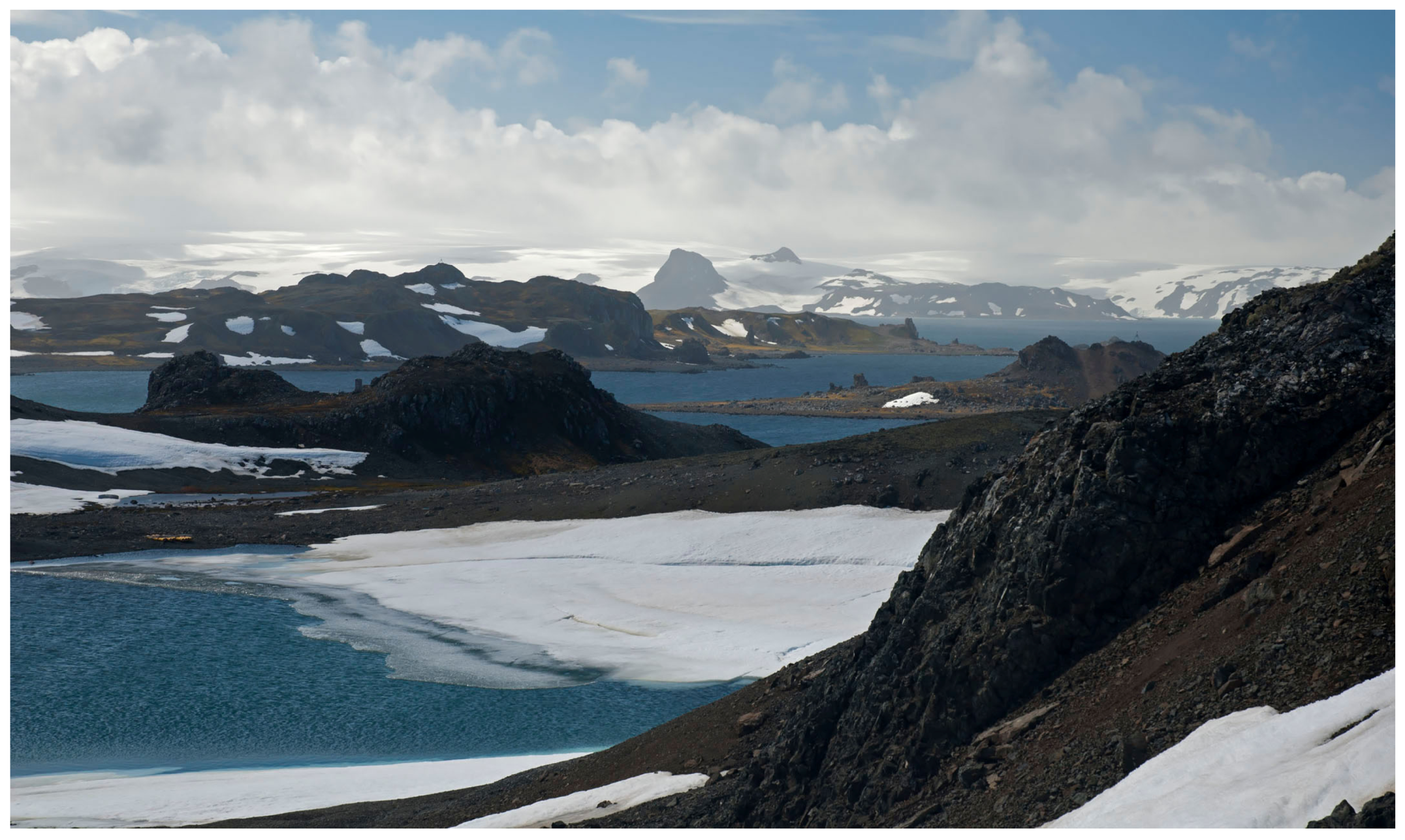
2.1. Study Area
2.2. Field Spectral Measurements
2.3. Discrimination between Cover Classes
3. Results
4. Discussion
5. Conclusions
Acknowledgments
Author Contributions
Conflicts of Interest
References
- Turner, J.; Barrand, N.E.; Bracegirdle, T.J.; Convey, P.; Hodgson, D.A.; Jarvis, M.; Jenkins, A.; Marshall, G.; Meredith, M.P.; Roscoe, H.; et al. Antarctic climate change and the environment: An update. Polar Rec. 2014, 50, 237–259. [Google Scholar] [CrossRef]
- Hughes, K.A.; Convey, P. Determining the native/non-native status of newly discovered terrestrial and freshwater species in Antarctica—Current knowledge, methodology and management action. J. Environ. Manag. 2012, 93, 52–66. [Google Scholar] [CrossRef] [PubMed]
- Hughes, K.A.; Pertierra, L.R.; Molina-Montenegro, M.A.; Convey, P. Biological invasions in terrestrial Antarctica: What is the current status and can we respond? Biodivers. Conserv. 2015, 24, 1031–1055. [Google Scholar] [CrossRef]
- Tin, T.; Fleming, Z.L.; Hughes, K.A.; Ainley, D.G.; Convey, P.; Moreno, C.A.; Pfeiffer, S.; Scott, J.; Snape, I. Impacts of local human activities on the Antarctic environment. Antarct. Sci. 2009, 21, 3–33. [Google Scholar] [CrossRef] [Green Version]
- Turner, J.; Bindschadler, R.; Convey, P.; di Prisco, G.; Fahrbach, E.; Gutt, J.; Hodgson, D.; Mayewski, P.; Summerhayes, C. (Eds.) Antarctic Climate Change and the Environment; Scientific Committee on Antarctic Research: Cambridge, UK, 2009.
- Favero-Longo, S.E.; Worland, M.R.; Convey, P.; Smith, R.I.L.; Piervittori, R.; Guglielmin, M.; Cannone, N. Primary succession of lichen and bryophyte communities following glacial recession on Signy Island, South Orkney Islands, Maritime Antarctic. Antarct. Sci. 2012, 24, 323–336. [Google Scholar] [CrossRef] [Green Version]
- Boy, J.; Godoy, R.; Shibistova, O.; Boy, D.; McCulloch, R.; de la Fuente, A.A.; Morales, M.A.; Mikutta, R.; Guggenberger, G. Successional patterns along soil development gradients formed by glacier retreat in the Maritime Antarctic, King George Island. Rev. Chil. Hist. Nat. 2016, 89, 6. [Google Scholar] [CrossRef]
- Gerighausen, U.; Brautigam, K.; Mustafa, O.; Peter, H.U. Expansion of vascular plants on an Antarctic island a consequence of climate change? In Antarctic Biology in a Global Context; Blackhuys Publishers: Leiden, The Netherlands, 2003; pp. 79–83. [Google Scholar]
- Convey, P.; Hopkins, D.W.; Roberts, S.J.; Tyler, A.N. Global southern limit of flowering plants and moss peat accumulation. Polar Res. 2011, 30, 157–171. [Google Scholar] [CrossRef]
- Frenot, Y.; Chown, S.L.; Whinam, J.; Selkirk, P.M.; Convey, P.; Skotnicki, M.; Bergstrom, D.M. Biological invasions in the Antarctic: Extent, impacts and implications. Biol. Rev. 2005, 80, 45–72. [Google Scholar] [CrossRef] [PubMed]
- Kennedy, A.D. Antarctic terrestrial ecosystem response to global environmental-change. Annu. Rev. Ecol. Syst. 1995, 26, 683–704. [Google Scholar] [CrossRef]
- Convey, P. Maritime antarctic climate change: Signals from terrestrial biology. In Antarctic Peninsula Climate Variability: Historical and Palaeo-Environmental Perspectives; Antarctic Research Series, American Geophysical Union: Washington, DC, USA, 2003; Volume 79, pp. 145–158. [Google Scholar]
- Callaghan, T.V.; Jonasson, S. Arctic terrestrial ecosystems and environmental-change. Philos. Trans. R. Soc. Lond. A Math. Phys. Eng. Sci. 1995, 352, 259–276. [Google Scholar] [CrossRef]
- Freckman, D.W.; Virginia, R.A. Low-diversity Antarctic soil nematode communities: Distribution and response to disturbance. Ecology 1997, 78, 363–369. [Google Scholar] [CrossRef]
- Smith, R.I.L. Vascular plants as bioindicators of regional warming in Antarctica. Oecologia 1994, 99, 322–328. [Google Scholar] [CrossRef]
- Green, T.G.A.; Sancho, L.G.; Pintado, A.; Schroeter, B. Functional and spatial pressures on terrestrial vegetation in Antarctica forced by global warming. Polar Biol. 2011, 34, 1643–1656. [Google Scholar] [CrossRef]
- Vieira, G.; Mora, C.; Pina, P.; Schaefer, C.E.R. A proxy for snow cover and winter ground surface cooling: Mapping Usnea sp communities using high-resolution remote sensing imagery (Maritime Antarctica). Geomorphology 2014, 225, 69–75. [Google Scholar] [CrossRef]
- Schmidt, K.S.; Skidmore, A.K. Spectral discrimination of vegetation types in a coastal wetland. Remote Sens. Environ. 2003, 85, 92–108. [Google Scholar] [CrossRef]
- Mendez-Rial, R.; Calvino-Cancela, M.; Martin-Herrero, J. Accurate implementation of anisotropic diffusion in the hypercube. IEEE Geosci. Remote Sens. Lett. 2010, 7, 870–874. [Google Scholar] [CrossRef]
- Mendez-Rial, R.; Calvino-Cancela, M.; Martin-Herrero, J. Anisotropic Inpainting of the Hypercube. IEEE Geosci. Remote Sens. Lett. 2012, 9, 214–218. [Google Scholar] [CrossRef]
- Buchhorn, M.; Walker, D.A.; Heim, B.; Raynolds, M.K.; Epstein, H.E.; Schwieder, M. Ground-based hyperspectral characterization of Alaska Tundra vegetation along environmental gradients. Remote Sens. 2013, 5, 3971–4005. [Google Scholar] [CrossRef] [Green Version]
- Fretwell, P.T.; Convey, P.; Fleming, A.H.; Peat, H.J.; Hughes, K.A. Detecting and mapping vegetation distribution on the Antarctic Peninsula from remote sensing data. Polar Biol. 2011, 34, 273–281. [Google Scholar] [CrossRef]
- Casanovas, P.; Black, M.; Fretwell, P.; Convey, P. Mapping lichen distribution on the Antarctic Peninsula using remote sensing, lichen spectra and photographic documentation by citizen scientists. Polar Res. 2015, 34, 25633. [Google Scholar] [CrossRef]
- Petzold, D.E.; Goward, S.N. Reflectance spectra of subarctic lichens. Remote Sens. Environ. 1988, 24, 481–492. [Google Scholar] [CrossRef]
- Shin, J.; Kim, H.; Kim, S.; Hong, S. Vegetation abundance on the Barton Peninsula, Antarctica: Estimation from high-resolution satellite images. Polar Biol. 2014, 37, 1579–1588. [Google Scholar] [CrossRef]
- Zhang, J.; Rivard, B.; Sánchez-Azofeifa, A. Spectral unmixing of normalized reflectance data for the deconvolution of lichen and rock mixtures. Remote Sens. Environ. 2005, 95, 57–66. [Google Scholar] [CrossRef]
- Margules, C.R.; Pressey, R.L. Systematic conservation planning. Nature 2000, 405, 243–253. [Google Scholar] [CrossRef] [PubMed]
- Chown, S.L.; Convey, P. Spatial and temporal variability across life’s hierarchies in the terrestrial Antarctic. Philos. Trans. R. Soc. Lond. B Biol. Sci. 2007, 362, 2307–2331. [Google Scholar] [CrossRef] [PubMed]
- Guglielmin, M.; Vieira, G. Permafrost and periglacial research in Antarctica: New results and perspectives. Geomorphology 2014, 225, 1–3. [Google Scholar] [CrossRef]
- Verhoef, W.; Bach, H. Simulation of hyperspectral and directional radiance images using coupled biophysical and atmospheric radiative transfer models. Remote Sens. Environ. 2003, 87, 23–41. [Google Scholar] [CrossRef]
- Calvino-Cancela, M.; Mendez-Rial, R.; Reguera-Salgado, J.; Martin-Herrero, J. Alien Plant Monitoring with Ultralight Airborne Imaging Spectroscopy. PLoS ONE 2014, 9, e102381. [Google Scholar] [CrossRef] [PubMed]
- Adams, J.; Smith, M.; Gillespie, A. Imaging Spectroscopy: Interpretation Based on Spectral Mixture Analysis; Cambridge University Press: New York, NY, USA, 1993. [Google Scholar]
- Clasen, A.; Somers, B.; Pipkins, K.; Tits, L.; Segl, K.; Brell, M.; Kleinschmit, B.; Spengler, D.; Lausch, A.; Foerster, M. Spectral unmixing of forest crown Ccomponents at close range, airborne and simulated sentinel-2 and EnMAP spectral imaging scale. Remote Sens. 2015, 7, 15361–15387. [Google Scholar] [CrossRef]
- Lee, B.; Won, Y.; Oh, S. Meteorological Characteristics at King Sejong Station, Antarctica (1988–1996); Report BSPE 97604-00-1020-7; Korea Ocean and Developmental Institute: Ansan, Korea, 1997; pp. 571–599. [Google Scholar]
- Chung, H.; Kim, J.H.; Lee, B.Y.; Keun, C.S.; Kim, Y. Ice cliff retreat and sea-ice formation observed around King Sejong Station in King George Island, West Antarctica. Ocean Polar Res. 2004, 26, 1–10. [Google Scholar] [CrossRef]
- Kim, J.H.; Ahn, I.Y.; Hong, S.G.; Andreev, M.; Lim, K.M.; Oh, M.J.; Koh, Y.J.; Hur, J.S. Lichen flora around the Korean Antarctic Scientific Station, King George Island, Antarctic. J. Microbiol. 2006, 44, 480–491. [Google Scholar] [PubMed]
- Kim, J.H.; Ahn, I.Y.; Lee, K.S.; Chung, H.; Choi, H.G. Vegetation of Barton Peninsula in the neighbourhood of King Sejong Station (King George Island, Maritime Antarctic). Polar Biol. 2007, 30, 903–916. [Google Scholar] [CrossRef]
- Kiedron, P.; Berndt, J.; Michalsky, J.; Harrison, L. Column water vapor from diffuse irradiance. Geophys. Res. Lett. 2003, 30, 1565. [Google Scholar] [CrossRef]
- vstedal, D.; Lewis Smith, R. Lichens of Antarctica and South Georgia: A Guide to Their Identification and Ecology; Cambridge University Press: Cambridge, UK, 2001. [Google Scholar]
- Ochyra, R.; Lewis Smith, R.; Bednarek-Ochyra, H. The Illustrated Moss Flora of Antarctica; Cambridge University Press: Cambridge, UK, 2008. [Google Scholar]
- Lee, Y.I.; Lim, H.S.; Yoon, H.I. Geochemistry of soils of King George Island, South Shetland Islands, West Antarctica: Implications for pedogenesis in cold polar regions. Geochim. Cosmochim. Acta 2004, 68, 4319–4333. [Google Scholar] [CrossRef]
- Ferreiro-Arman, M.; Da Costa, J.P.; Homayouni, S.; Martín-Herrero, J. Hyperspectral Image Analysis for Precision Viticulture. In Image Analysis and Recognition, Part II; Lecture Notes in Computer Science; Campilho, A., Kamel, M., Eds.; Springer: Berlin/Heidelberg, Germany, 2006; Volume 4142, pp. 730–741. [Google Scholar]
- Song, S.; Gong, W.; Zhu, B.; Huang, X. Wavelength selection and spectral discrimination for paddy rice, with laboratory measurements of hyperspectral leaf reflectance. ISPRS J. Photogramm. Remote Sens. 2011, 66, 672–682. [Google Scholar] [CrossRef]
- Asner, G.P.; Martin, R.E.; Bin Suhaili, A. Sources of canopy chemical and spectral diversity in Lowland Bornean Forest. Ecosystems 2012, 15, 504–517. [Google Scholar] [CrossRef]
- Lehmann, J.R.K.; Grosse-Stoltenberg, A.; Roemer, M.; Oldeland, J. Field Spectroscopy in the VNIR-SWIR Region to discriminate between mediterranean native plants and exotic-invasive Shrubs based onleaf tannin Content. Remote Sens. 2015, 7, 1225–1241. [Google Scholar] [CrossRef] [Green Version]
- Cohen, J. A Coefficient of Agreement for nominal scales. Educ. Psychol. Meas. 1960, 20, 37–46. [Google Scholar] [CrossRef]
- Landis, J.R.; Koch, G.G. Measurement of observer agreement for categorical data. Biometrics 1977, 33, 159–174. [Google Scholar] [CrossRef] [PubMed]
- Congalton, R.G.; Oderwald, R.G.; Mead, R.A. Assessing Landsat classification accuracy using discrete multivariate statistical techniques. Photogramm. Eng. Remote Sens. 1983, 49, 1671–1678. [Google Scholar]
- Kohonen, T. Self-organized formation of topologically correct feature maps. Biol. Cybern. 1982, 43, 59–69. [Google Scholar] [CrossRef]
- Kohonen, T. The self-organizing map. Proc. IEEE 1990, 78, 1464–1480. [Google Scholar] [CrossRef]
- Martín-Herrero, J.; Ferreiro-Arman, M.; Alba-Castro, J. Grading textured surfaces with automated soft clustering in a supervised SOM. In Image Analysis and Recognition, Part II; Lecture Notes in Computer Science; Campilho, A., Kamel, M., Eds.; Springer: Berlin/Heidelberg, Germany, 2004; Volume 3212, pp. 323–330. [Google Scholar]
- Aymerich, I.F.; Oliva, M.; Giralt, S.; Martín-Herrero, J. Detection of Tephra Layers in Antarctic Sediment Cores with Hyperspectral Imaging. PLoS ONE 2016, 11, e0146578. [Google Scholar] [CrossRef] [PubMed]
- Bechtel, R.; Rivard, B.; Sánchez-Azofeifa, A. Spectral properties of foliose and crustose lichens based on laboratory experiments. Remote Sens. Environ. 2002, 82, 389–396. [Google Scholar] [CrossRef]
- Rees, W.; Tutubalina, O.; Golubeva, E. Reflectance spectra of subarctic lichens between 400 and 2400 nm. Remote Sens. Environ. 2004, 90, 281–292. [Google Scholar] [CrossRef]
- Tucker, C.J. Red and photographic infrared linear combinations for monitoring vegetation. Remote Sens. Environ. 1979, 8, 127–150. [Google Scholar] [CrossRef]
- Ceccato, P.; Flasse, S.; Tarantola, S.; Jacquemoud, S.; Gregoire, J.M. Detecting vegetation leaf water content using reflectance in the optical domain. Remote Sens. Environ. 2001, 77, 22–33. [Google Scholar] [CrossRef]
- Ayala-Silva, T.; Beyl, C.A. Changes in spectral reflectance of wheat leaves in response to specific macronutrient deficiency. Adv. Space Res. 2005, 35, 305–317. [Google Scholar] [CrossRef] [PubMed]
- Liu, L.Y.; Wang, J.H.; Huang, W.J.; Zhao, C.J.; Zhang, B.; Tong, Q.X. Estimating winter wheat plant water content using red edge parameters. Int. J. Remote Sens. 2004, 25, 3331–3342. [Google Scholar] [CrossRef]
- Pertierra, L.R.; Lara, F.; Tejedo, P.; Quesada, A.; Benayas, J. Rapid denudation processes in cryptogamic communities from Maritime Antarctica subjected to human trampling. Antarct. Sci. 2013, 25, 318–328. [Google Scholar] [CrossRef]
- Favero-Longo, S.E.; Cannone, N.; Worland, M.R.; Convey, P.; Piervittori, R.; Guglielmin, M. Changes in lichen diversity and community structure with fur seal population increase on Signy Island, South Orkney Islands. Antarct. Sci. 2011, 23, 65–77. [Google Scholar] [CrossRef]
- Sancho, L.G.; Valladares, F. Lichen colonization of recent moraines on Livingston Island (South Shetland, Antarctica). Polar Biol. 1993, 13, 227–233. [Google Scholar] [CrossRef]


| Class | Brief Description |
|---|---|
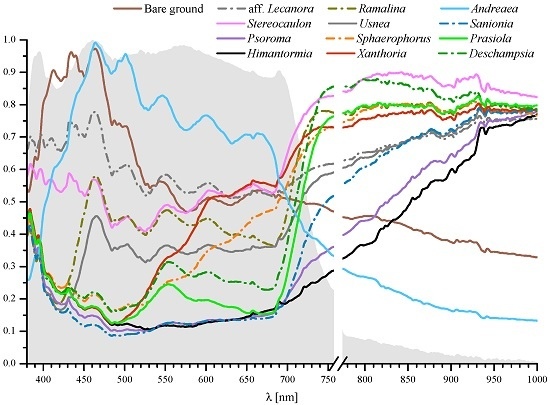
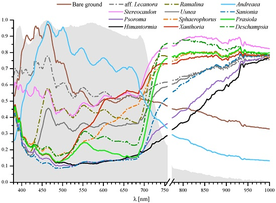
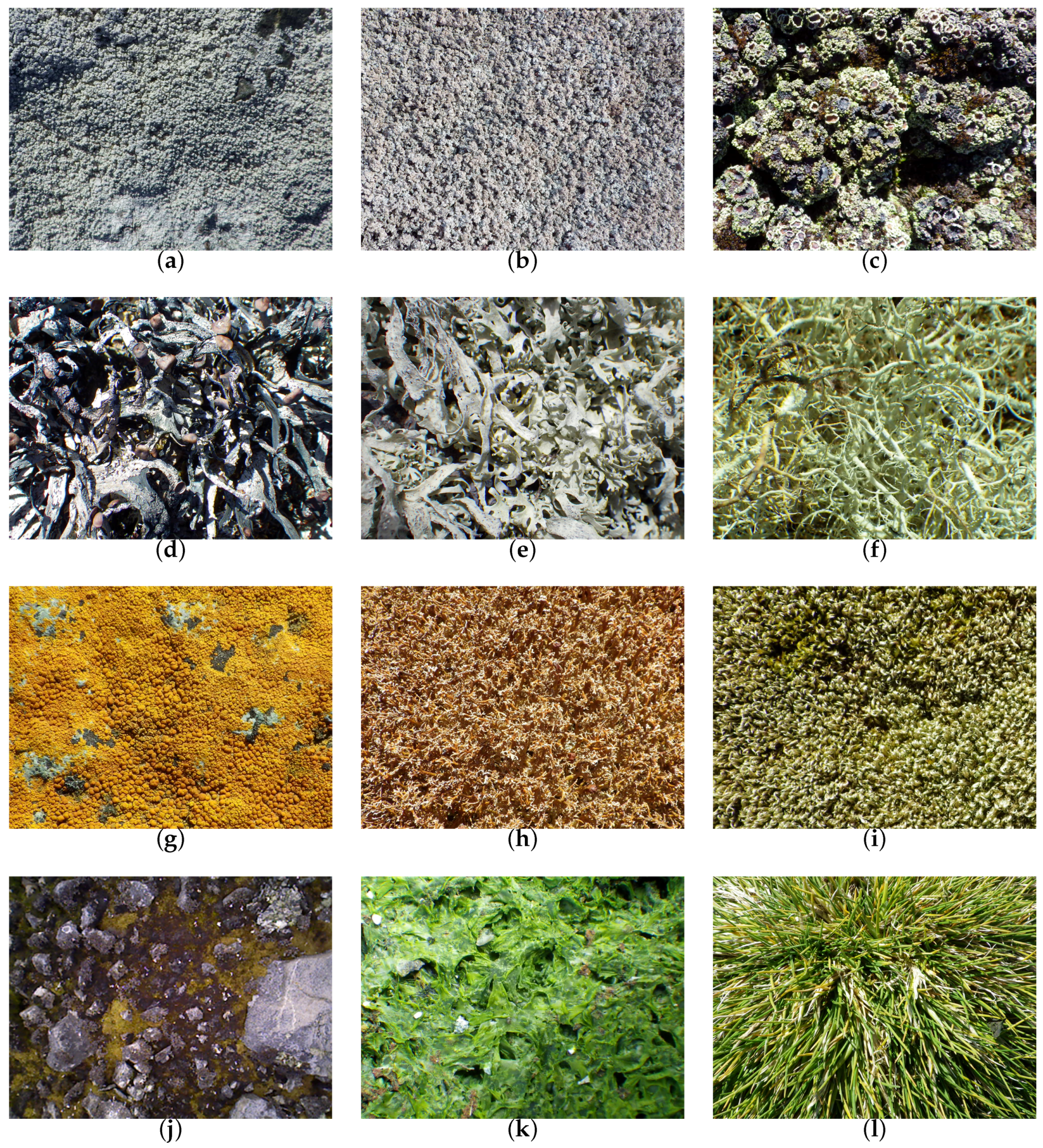
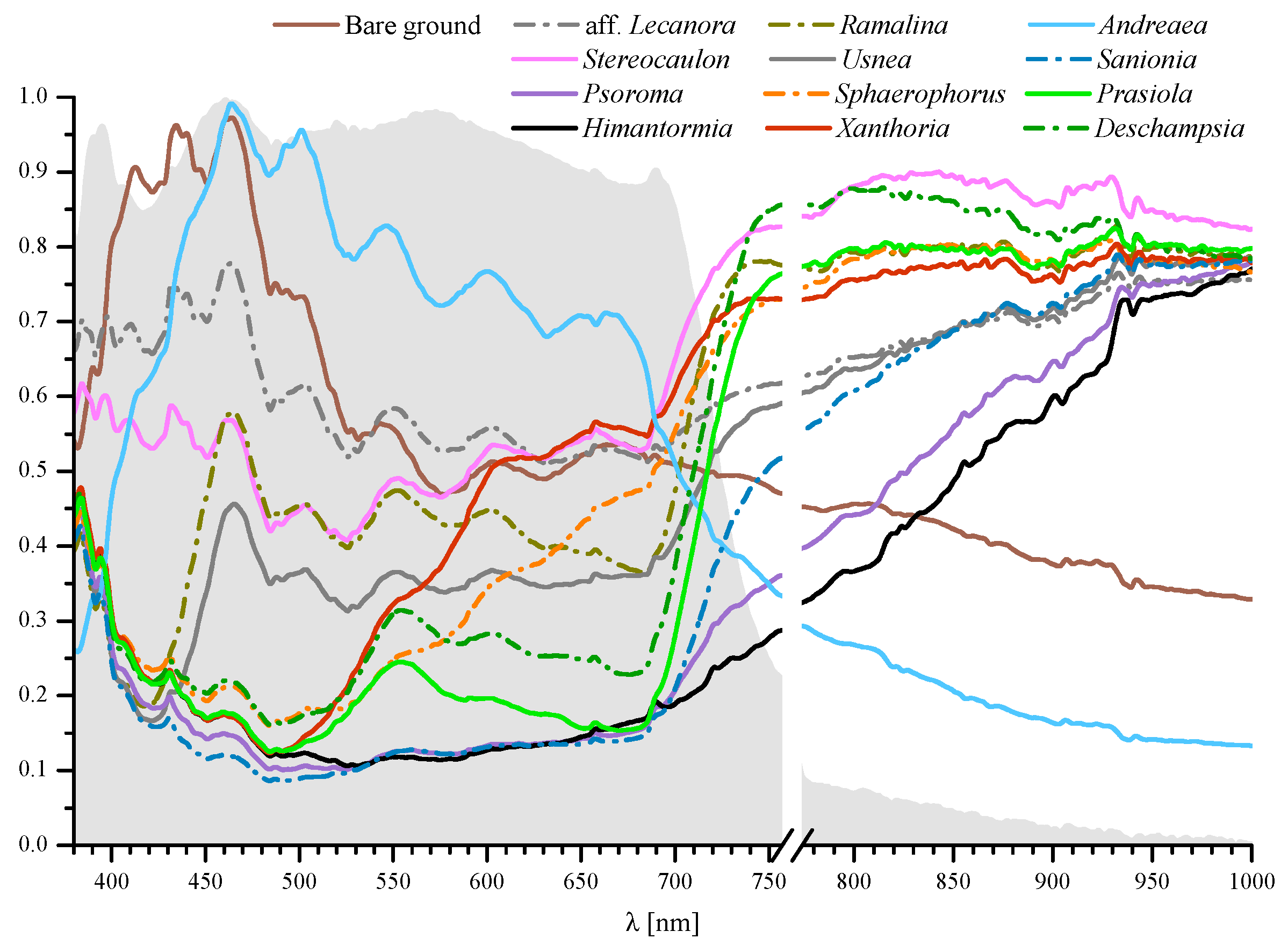
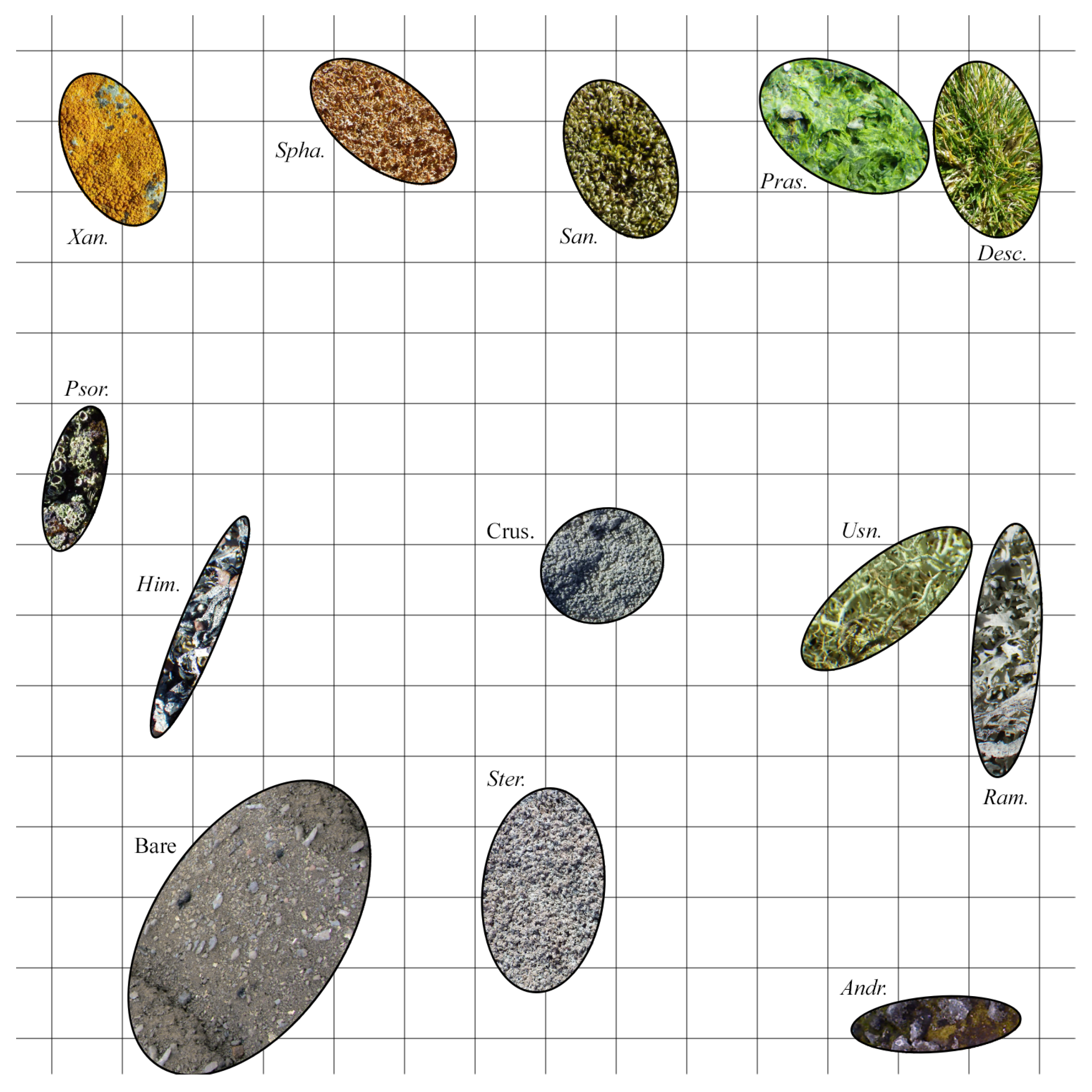
| Bare ground | Ground with no macroscopic forms of vegetation. Soils in the Barton Peninsula are generally poor in organic material and nutrients and mostly composed of mineral and rock fragments derived from the bedrock and volcanic ashes. Samples were taken in basaltic andesite areas. |
| Lichens | |
| Aff. Lecanora polytropa | Crustose growth form with aerolate thallus, common on rocks frequented by birds. |
| Stereocaulon sp. | Fruticose growth form with photobiont trebouxioid and cephalodia containing cyanobacteria. |
| Psoroma sp. | Squamulose growth form with photobiont Myrmecia and cephalodia containing Nostoc. Frequently growing on mosses. |
| Himantormia lugubris | Fruticose growth form and a trebouxioid photobiont. Endemic to Antarctica. |
| Ramalina aff. tenebrata | Fruticose growth form containing usnic acid. Widespread on coastal cliffs and large boulders frequently associated with bird colonies (ornithocoprohillous). |
| Usnea antarctica | Fruticose lichen with probably the widest ecological amplitude of any Antarctic lichen. Abundant in most habitats from sheltered to very exposed and moist to dry situations. It forms dense stands on pebbles and gravels. Common and locally abundant on mosses. |
| Xanthoria sp. | Foliose growth form rich in anthraquinone pigment giving its characteristic orange colour. Abundant on rocks influenced by birds. |
| Sphaerophorus globosus | Fruticose lichen growing in coralloid tufts to 10 cm tall. Photobiont trebouxioid. |
| Mosses | |
| Sanionia uncinata | Mat forming moss with a wide geographic distribution and growing in a variety of substrata. |
| Andreaea sp. | Pioneer moss in exposed rocks and fellfields. The spectra recorded correspond to mixtures of rocks (basaltic andesite) and Andreaea mosses, both alive and dead. |
| Alga | |
| Prasiola crispa | Nitrophilous alga that forms dense mats in wet areas very high in nutrients in penguin colonies. |
| Vascular plant | |
| Deschampsia antarctica | One of the two flowering plants native to Antarctica. Cushion-forming perennial grass with thin leaves. |
| PC | Variance | Λ | F | df | P |
|---|---|---|---|---|---|
| #1 | 57.9% | 0.017 | 1826.114 | 12, 377 | <0.001 |
| #2 | 32.5% | 0.195 | 129.428 | 12, 377 | <0.001 |
| #3 | 4.9 % | 0.089 | 322.444 | 12, 377 | <0.001 |
| #4 | 2.5% | 0.093 | 306.053 | 12, 377 | <0.001 |
| #5 | 1.7% | 0.068 | 431.742 | 12, 377 | <0.001 |
| Pred. | Bare | Crus. | Ster. | Ram. | Usn. | Psor. | Him. | Spha. | Xan. | Andr. | San. | Desc. | Pras. | Prod. | User | |
|---|---|---|---|---|---|---|---|---|---|---|---|---|---|---|---|---|
| True | ||||||||||||||||
| Bare ground | 30 | 0 | 0 | 0 | 0 | 0 | 0 | 0 | 0 | 0 | 0 | 0 | 0 | 100% | 100% | |
| Crus. aff. Lec. | 0 | 30 | 0 | 0 | 0 | 0 | 0 | 0 | 0 | 0 | 0 | 0 | 0 | 100% | 100% | |
| Stereocaulon | 0 | 0 | 30 | 0 | 0 | 0 | 0 | 0 | 0 | 0 | 0 | 0 | 0 | 100% | 100% | |
| Ramalina | 0 | 0 | 0 | 29 | 1 | 0 | 0 | 0 | 0 | 0 | 0 | 0 | 0 | 96.7% | 87.9% | |
| Usnea | 0 | 0 | 0 | 4 | 26 | 0 | 0 | 0 | 0 | 0 | 0 | 0 | 0 | 86.7% | 96.3% | |
| Psoroma | 0 | 0 | 0 | 0 | 0 | 30 | 0 | 0 | 0 | 0 | 0 | 0 | 0 | 100% | 96.8% | |
| Himantormia | 0 | 0 | 0 | 0 | 0 | 0 | 30 | 0 | 0 | 0 | 0 | 0 | 0 | 100% | 100% | |
| Sphaerophorus | 0 | 0 | 0 | 0 | 0 | 1 | 0 | 24 | 2 | 0 | 3 | 0 | 0 | 80.0% | 100% | |
| Xanthoria | 0 | 0 | 0 | 0 | 0 | 0 | 0 | 0 | 30 | 0 | 0 | 0 | 0 | 100% | 93.8% | |
| Andreaea | 0 | 0 | 0 | 0 | 0 | 0 | 0 | 0 | 0 | 30 | 0 | 0 | 0 | 100% | 100% | |
| Sanionia | 0 | 0 | 0 | 0 | 0 | 0 | 0 | 0 | 0 | 0 | 28 | 0 | 2 | 93.3% | 82.4% | |
| Deschampsia | 0 | 0 | 0 | 0 | 0 | 0 | 0 | 0 | 0 | 0 | 0 | 22 | 8 | 73.3% | 73.3% | |
| Prasiola | 0 | 0 | 0 | 0 | 0 | 0 | 0 | 0 | 0 | 0 | 3 | 8 | 19 | 63.3% | 65.5% | |
| Pred. | Bare | Crus. | Ster. | Ram. | Usn. | Psor. | Him. | Spha. | Xan. | Andr. | San. | Desc. | Pras. | Prod. | User | |
|---|---|---|---|---|---|---|---|---|---|---|---|---|---|---|---|---|
| True | ||||||||||||||||
| Bare ground | 30 | 0 | 0 | 0 | 0 | 0 | 0 | 0 | 0 | 0 | 0 | 0 | 0 | 100% | 100% | |
| Crus. aff. Lec. | 0 | 30 | 0 | 0 | 0 | 0 | 0 | 0 | 0 | 0 | 0 | 0 | 0 | 100% | 100% | |
| Stereocaulon | 0 | 0 | 30 | 0 | 0 | 0 | 0 | 0 | 0 | 0 | 0 | 0 | 0 | 100% | 100% | |
| Ramalina | 0 | 0 | 0 | 29 | 1 | 0 | 0 | 0 | 0 | 0 | 0 | 0 | 0 | 96.7% | 87.9% | |
| Usnea | 0 | 0 | 0 | 4 | 26 | 0 | 0 | 0 | 0 | 0 | 0 | 0 | 0 | 86.7% | 96.3% | |
| Psoroma | 0 | 0 | 0 | 0 | 0 | 30 | 0 | 0 | 0 | 0 | 0 | 0 | 0 | 100% | 96.8% | |
| Himantormia | 0 | 0 | 0 | 0 | 0 | 0 | 30 | 0 | 0 | 0 | 0 | 0 | 0 | 100% | 100% | |
| Sphaerophorus | 0 | 0 | 0 | 0 | 0 | 1 | 0 | 24 | 2 | 0 | 3 | 0 | 0 | 80.0% | 100% | |
| Xanthoria | 0 | 0 | 0 | 0 | 0 | 0 | 0 | 0 | 30 | 0 | 0 | 0 | 0 | 100% | 93.8% | |
| Andreaea | 0 | 0 | 0 | 0 | 0 | 0 | 0 | 0 | 0 | 30 | 0 | 0 | 0 | 100% | 100% | |
| Sanionia | 0 | 0 | 0 | 0 | 0 | 0 | 0 | 0 | 0 | 0 | 28 | 0 | 2 | 93.3% | 82.4% | |
| Deschampsia | 0 | 0 | 0 | 0 | 0 | 0 | 0 | 0 | 0 | 0 | 0 | 21 | 9 | 70.0% | 70.0% | |
| Prasiola | 0 | 0 | 0 | 0 | 0 | 0 | 0 | 0 | 0 | 0 | 3 | 9 | 18 | 60.0% | 62.1% | |
© 2016 by the authors; licensee MDPI, Basel, Switzerland. This article is an open access article distributed under the terms and conditions of the Creative Commons Attribution (CC-BY) license (http://creativecommons.org/licenses/by/4.0/).
Share and Cite
Calviño-Cancela, M.; Martín-Herrero, J. Spectral Discrimination of Vegetation Classes in Ice-Free Areas of Antarctica. Remote Sens. 2016, 8, 856. https://doi.org/10.3390/rs8100856
Calviño-Cancela M, Martín-Herrero J. Spectral Discrimination of Vegetation Classes in Ice-Free Areas of Antarctica. Remote Sensing. 2016; 8(10):856. https://doi.org/10.3390/rs8100856
Chicago/Turabian StyleCalviño-Cancela, María, and Julio Martín-Herrero. 2016. "Spectral Discrimination of Vegetation Classes in Ice-Free Areas of Antarctica" Remote Sensing 8, no. 10: 856. https://doi.org/10.3390/rs8100856