An Approach to Extended Fresnel Scattering for Modeling of Depolarizing Soil-Trunk Double-Bounce Scattering

Abstract

Focusing on scattering from natural media, dihedral (double bounce) scattering is often characterized as a soil-trunk double Fresnel reflection, like for instance, in most model-based decompositions. As soils are predominantly rough in agriculture, the classical Rank 1 dihedral scattering component has to be extended to account for soil roughness-induced depolarization. Therefore, an azimuthal Line of Sight (LoS) rotation is applied solely on the soil plane of the double-bounce reflection to generate a depolarized dihedral scattering signal in agriculture. The results of the sensitivity analysis are shown for a distributed target in coherency matrix representation. It reveals that the combination of coherency matrix elements T_22XD + T_33XD is quasi-independent of the roughness-induced depolarization, while (T_22XD − T_33XD)/(T_22XD + T_33XD) is quasi-independent of the dielectric properties of the reflecting media. Therefore, a depolarization-independent retrieval of soil moisture or a direct roughness retrieval from the extended dihedral scattering component might be possible in stalk-dominated agriculture under certain conditions (e.g., the influence of a differential phase stays at a low level: ϕ < 15°). The first analyses with L-band airborne-SAR data of DLR’s E-SAR and F-SAR systems in agricultural regions during the AgriSAR, OPAQUE, SARTEO and TERENO project campaigns state the existence and potential of the extended Fresnel scattering mechanism to represent dihedral scattering between a rough (tilled) soil and the stalks of the agricultural plants.

1. Introduction

The increasing availability of fully-polarimetric datasets from space-borne SAR systems like ALOS-1/-2, Radarsat-2, TerraSAR-X and TanDEM-X motivates the investigation of polarimetric scattering mechanisms for natural media [1,2,3,4,5,6,7]. As natural media are mostly distributed scatterers, assuming more than one scatterer within the resolution cell, mathematical notations including second order statistics, like the coherency matrix [T], are needed for a complete description of the polarimetric scattering scenario [8]. As mostly more than one dominant scattering process is occurring within the resolution cell, polarimetric decompositions are one option to analyze the different scattering components.

There are two common ways mainly published in the literature to decompose fully-polarimetric data represented by [T] [8,9] Eigen-based and model-based decompositions. The Eigen-based methods represent a mathematical approach for decomposition, which result in a set of eigenvalues and eigenvectors [9,10]. These parameters are not straightforward to interpret in their physical sense. The model-based decompositions, on the contrary, consist of simple, physically-based electro-magnetic scattering models, which are easy to interpret in terms of scattering physics, but have to be pre-defined by at least some a priori knowledge [11,12]. One of the most popular configurations for a standard three-component, model-based polarimetric decomposition for natural media consists of a surface component, a dihedral component and a volume component [13]. Hajnsek et al. [14] showed how to incorporate Rank 3 extended Bragg surface scattering into the surface component in order to account for roughness-induced depolarization on agricultural ground. This is of special importance for agricultural areas, where the soil roughness is distinct and cannot be neglected. Similarly, a dihedral scattering component will be developed in Section 2, which also accounts for roughness-induced depolarization, because up to now, predominantly smooth double Fresnel scattering is used in standard decompositions [11,13,14]. A sensitivity analysis for the coherency matrix elements on the dielectric content of the soil and the trunk plane, the differential phase, the loss factor, as well as on the local incidence angle is given in Section 3. The appearance of extended Fresnel scattering in agriculture is investigated in Section 4 using fully-polarimetric, airborne SAR data. The potentials and limitations of this novel, depolarizing, scattering component are discussed in Section 5 followed by a summary and the first conclusions in Section 6.

2. Development of the Extend Fresnel Scattering Model

2.1. Rank 1 Fresnel Scattering

The canonical dihedral component is expressed as a double reflection occurring at each of two smooth, orthogonal planes of a dihedral scatterer [8]. Therefore, the dihedral scattering matrix of a soil-trunk reflection (assuming flat ground and stalk-dominated vegetation arranged in dense rows) is modeled as:

$$\left[S_D\right]=\left[\begin{array}{cc}{R}_{Hs}{R}_{Ht}({\omega }_l,{\epsilon }_S,{\epsilon }_T)& 0\\ 0& -R_{Vs}{R}_{Vt}{e}^{i\phi }({\omega }_l,{\epsilon }_S,{\epsilon }_T)\end{array}\right]$$

(1)

R_Hs and R_Vs are the horizontal and vertical Fresnel coefficients of the soil scattering plane, which depend on the dielectric constant of the soil ε_s and the local incidence angle ω_l [8]:

$$R_{Hs}=\frac{\cos {\omega }_l-\sqrt{{\epsilon }_s-{\sin }^2{\omega }_l}}{\cos {\omega }_l+\sqrt{{\epsilon }_s-{\sin }^2{\omega }_l}}, R_{Vs}=\frac{{\epsilon }_s\cos {\omega }_l-\sqrt{{\epsilon }_s-{\sin }^2{\omega }_l}}{{\epsilon }_s\cos {\omega }_l+\sqrt{{\epsilon }_s-{\sin }^2{\omega }_l}}$$

(2)

R_Ht and R_Vt are the Fresnel coefficients of the trunk scattering plane, which include the dielectric constant of the trunk ε_t and the local incidence angle ω_l [8]. For modelling reasons, it is assumed that the vertical scattering plane is formed by the plant trunks planted densely in seeding rows.

$$R_{Ht}=\frac{\cos \left(\frac{\pi }{2}-{\omega }_l\right)-\sqrt{{\epsilon }_t-{\sin }^2\left(\frac{\pi }{2}-{\omega }_l\right)}}{\cos \left(\frac{\pi }{2}-{\omega }_l\right)+\sqrt{{\epsilon }_t-{\sin }^2\left(\frac{\pi }{2}-{\omega }_l\right)}}, R_{Vt}=\frac{{\epsilon }_t\cos \left(\frac{\pi }{2}-{\omega }_l\right)-\sqrt{{\epsilon }_t-{\sin }^2\left(\frac{\pi }{2}-{\omega }_l\right)}}{{\epsilon }_t\cos \left(\frac{\pi }{2}-{\omega }_l\right)+\sqrt{{\epsilon }_t-{\sin }^2\left(\frac{\pi }{2}-{\omega }_l\right)}}$$

(3)

The phase angle φ within the factor $e^{i\varphi }$ accounts for the phase difference between the HH- and VV-polarization backscatter incorporated, if propagation through oriented media occurs (further details in [15]). The Pauli scattering vector is obtained as [8,9]:

$${\overrightarrow{k}}_D=\frac{1}{\sqrt{2}}{\left[R_{Hs}{R}_{Ht}-R_{Vs}{R}_{Vt}{e}^{i\phi },R_{Hs}{R}_{Ht}+R_{Vs}{R}_{Vt}{e}^{i\phi },0\right]}^T$$

(4)

$$\langle \left[T_D\right]\rangle =\langle {\overrightarrow{k}}_D\cdot {\overrightarrow{k}}_D^{+}\rangle =f_d\left[\begin{array}{ccc}{\left|{\alpha }_D\right|}^2& {\alpha }_D& 0\\ {\alpha }_D{}^{*}& 1& 0\\ 0& 0& 0\end{array}\right]$$

(5)

The resulting coherency matrix [T_D] follows as derived in [13] and is parameterized by the complex scattering mechanism ratio α_D and the real backscattering amplitude f_D [14]:

$${\alpha }_D=\frac{R_{Hs}{R}_{Ht}-R_{Vs}{R}_{Vt}{e}^{i\phi }}{R_{Hs}{R}_{Ht}+R_{Vs}{R}_{Vt}{e}^{i\phi }}{f}_D=\frac{1}{2}{\left|R_{Hs}{R}_{Ht}+R_{Vs}{R}_{Vt}{e}^{i\phi }\right|}^2$$

(6)

In addition, the power P_D is represented by the trace of [T_D]: P_D = f_D (1 + |α_D|²).

As the dihedral scattering model assumes two specular reflections on each of the two orthogonal planes, the model is adapted subsequently for application on natural, respectively lossy, surfaces. Thus, the loss due to scattering at the soil plane is considered by a scattering loss factor L_S [11,16]:

$$\mathrm{Gaussian}: L_S=\exp (-2\cdot k^2\cdot {\sigma }^2\cdot {\cos }^2{\omega }_l)$$

(7)

$$\mathrm{Exponential}: L_S=\exp (-2\cdot k\cdot \sigma \cdot \cos {\omega }_l)$$

(8)

where k is the wave number, σ the standard deviation of the vertical roughness of the soil and ω_l is the local incidence angle [12]. The Fresnel coefficients of the soil scatterer (R_Hs, R_Vs) are altered to the so-called modified Fresnel coefficients (RL_Hs, RL_Vs) accordingly [11]:

$$\begin{array}{l}R{L}_{Hs}=R_{Hs}\times L_S\\ R{L}_{Vs}=R_{Vs}\times L_S\end{array}$$

(9)

The complex ratio α_D is independent of the scattering loss factor L_S, because the multiplicative factor cancels out. Thus, only the backscattering amplitude f_D is affected by the soil roughness loss. However, the roughness-induced depolarization is not included, which would also affect the complex ratio α_D [14].

$$\begin{array}{ll}{f}_{Dloss}& =\frac{1}{2}{\left|R_{Hs}{L}_s{R}_{Ht}+R_{Vs}{L}_s{R}_{Vt}{e}^{i\phi }\right|}^2=\frac{1}{2}{\left|L_S\cdot (R_{Hs}{R}_{Ht}+R_{Vs}{R}_{Vt}{e}^{i\phi })\right|}^2\\ & =f_D{\left|L_S\right|}^2\end{array}$$

(10)

Finally, the coherency matrix for the modified dihedral scattering contribution [T_DLoss] is written as [14]

$$\langle \left[T_{DLoss}\right]\rangle =f_D\cdot {\left|L_S\right|}^2\left[\begin{array}{ccc}{\left|{\alpha }_D\right|}^2& {\alpha }_D& 0\\ {\alpha }_D{}^{*}& 1& 0\\ 0& 0& 0\end{array}\right]$$

(11)

2.2. Rank 3 Extended Fresnel Scattering

In order to account for soil roughness-induced depolarization, a Line of Sight (LoS) rotation of θ, solely around the soil plane (R_Hs, R_Vs), is introduced in Equation (12). It is important to note that the rotation is only applied to the soil plane, like in Equation (12), while the trunk plane is assumed static (no trunk roughness) [12]. A conceptual visualization is given in Figure 1. Hence, the orientation of the vegetation volume is not a variable in this approach. Therefore, the assumption is made that the second dihedral scattering event (scattering center at the stalks/stems of the vegetation) is approximated as Fresnel scattering from a vertical plane. The orientation of the vegetation is expected to be located within this plane. Hence, only rotations perpendicular to the soil and to the incidence plane are assumed. Rotations would only matter as far as the vegetation structure forming the second plane reaches outside of this plane [17,18]. The double Fresnel reflection is a distinct assumption within the dihedral scattering component and represents a significant simplification of the scattering scenario. However, if only the soil plane of the dihedral scattering mechanism rotates, whereas the trunk one does not, backscattering is no more at specular direction. This is due to incoherent scattering from rough soil and coherent reflection by the trunk plane. For a non-rotated soil plane, we have coherent reflection from both rough soil, as well as trunk. Hence, the Fresnel coefficients can be used for any terrain roughness. Conversely, for a (only) rotated soil plane, its scattering is incoherent, and Bragg or Fresnel coefficients can be applied according to surface roughness: Bragg for small roughness; Fresnel for distinct roughness. The latter was adopted in the case of extended Fresnel scattering in agriculture. These simplifications are needed to keep the model complexity and the space of variables low. Eventually, the test with experimental SAR data in Section 4 will give the first indications if this novel scattering model can describe the data to a certain extent.

$$\left[S_{XD}\right]=\frac{L_{S_{XD}}}{2}\left(\begin{array}{l}\left(\left[\begin{array}{cc}1& 0\\ 0& -1\end{array}\right]\left[\begin{array}{cc}1& 0\\ 0& e^{i\phi }\end{array}\right]\left[\begin{array}{cc}Cos\theta & Sin\theta \\ -Sin\theta & Cos\theta \end{array}\right]\left[\begin{array}{cc}{R}_{Hs}& 0\\ 0& R_{Vs}\end{array}\right]{\left[\begin{array}{cc}Cos\theta & Sin\theta \\ -Sin\theta & Cos\theta \end{array}\right]}^T\left[\begin{array}{cc}{R}_{Ht}& 0\\ 0& R_{Vt}\end{array}\right]\right)+\\ \left(\left[\begin{array}{cc}{R}_{Ht}& 0\\ 0& R_{Vt}\end{array}\right]\left[\begin{array}{cc}Cos\theta & Sin\theta \\ -Sin\theta & Cos\theta \end{array}\right]\left[\begin{array}{cc}{R}_{Hs}& 0\\ 0& R_{Vs}\end{array}\right]{\left[\begin{array}{cc}Cos\theta & Sin\theta \\ -Sin\theta & Cos\theta \end{array}\right]}^T\left[\begin{array}{cc}1& 0\\ 0& e^{i\phi }\end{array}\right]\left[\begin{array}{cc}1& 0\\ 0& -1\end{array}\right]\right)\end{array}\right)$$

(12)

Equation (12) contains both possible ray paths to obtain reciprocity (see also Equation (10) in Dahon et al., [19]): soil-trunk reflection and trunk-soil reflection, respectively. Lee et al. published a depolarizing dihedral component, where both the soil and the trunk plane are rotated simultaneously by a LoS rotation of the dihedral coherency matrix [20]. However, the assumption of a trunk roughness (rotation around the trunk plane) in agriculture is physically hardly justifiable, as the stalks forming the trunk plane are supposed to be static during acquisition. In addition, Neumann and Al-Kahachi introduced the rotation solely around the vertical plane (forest trunks/methane bubbles in lake ice) in the dihedral component to model different forest vegetation (height >10 m)/ice components [21,22] at L-band. However, both approaches also increase the entropy of the trunk scattering and are not as closely related to the physical scattering mechanism of a rough soil and an agricultural plant (e.g., wheat stalks) as the proposed one. This might be present in agricultural areas (height < 3 m) at the L-band and will be investigated with real data in Section 4. Here, only a rough and depolarizing soil plane is assumed, modelled by an LoS rotation, and a smooth trunk plane (plant stalks). Hence, the rotated scattering matrix [S_XD] is presented as:

$$\left[S_{XD}\right]=L_{S_{XD}}\left[\begin{array}{cc}{R}_{Ht}(R_{Hs}{\cos }^2\theta +R_{Vs}{\sin }^2\theta )& \frac{1}{4}(R_{Vs}-R_{Hs})(R_{Vt}-R_{Ht}{e}^{i\phi })\sin 2\theta \\ \frac{1}{4}(R_{Vs}-R_{Hs})(R_{Vt}-R_{Ht}{e}^{i\phi })\sin 2\theta & -R_{Vt}{e}^{i\phi }(R_{Vs}{\cos }^2\theta +R_{Hs}{\sin }^2\theta )\end{array}\right]=L_{S_{XD}}\left[\begin{array}{cc}{S}_{XD11}& S_{XD12}\\ S_{XD21}& S_{XD22}\end{array}\right]$$

(13)

It can be seen that the model of extended Fresnel scattering fulfills the reciprocity theorem, which is obligatory for monostatic acquisition systems (S_XD12 = S_XD21). The Pauli scattering vector is formed in Equation (14) to account for distributed targets by calculating in the next step the coherency matrix [T_XD] from the outer product of the scattering vectors [10].

$${\overrightarrow{k}}_{XD}=\frac{L_{S_{XD}}}{\sqrt{2}}{\left[\begin{array}{ccc}{S}_{XD11}+S_{XD22}& S_{XD11}-S_{XD22}& S_{XD12}+S_{XD21}\end{array}\right]}^T$$

(14)

Within the formation of the coherency matrix in Equation (15), the angle accounting for the soil roughness is integrated over a rotation angle range from −θ₁ to θ₁ with a uniform probability function (pdf_θ = 1/(2θ₁)) representing the rotation limits (±θ₁) and probability distribution (pdf_θ) of the rotation angles of the soil plane [11]. Hence, the strength of the soil roughness-induced depolarization is steered by this rotation limit angle. The assumption of a uniform distribution width pays tribute to a randomly-oriented small-scale roughness, which is predominant for stalk-grown agricultural crops, where the seedbed (with more smooth soil conditions) was prepared during planting. Hence, major row structures from ploughing should not be present anymore, and therefore, a uniform distribution (more random distribution of soil roughness) seems likely to represent the true scattering case for seedbed conditions. It is not expected that certain roughness angles are of higher probability to occur than others, especially within the vegetation growing period in agriculture (after seedbed preparation). However, this is an assumption and can be adapted in the future to generalize the approach to different soil roughness cases. Anyway, as the pdf is a factorial term within the calculus of the coherency matrix elements (cf. Equation (15)), the ratios of coherency matrix elements will not be affected by a change of the probability density function.

After integration, the resulting coherency matrix [T_XD] is reflection symmetric, and subsequently, the off-diagonal elements T_XD13, T_XD23, T_XD31 and T_XD32 are zero.

$$\langle \left[T_{XD}\right]\rangle ={\left|L_{S_{XD}}\right|}^2\cdot {\displaystyle \underset{-{\theta }_1}{\overset{{\theta }_1}{\int }}{\overrightarrow{k}}_{XD}}\cdot {\overrightarrow{k}}_{XD}^{T*}\cdot pd{f}_{\theta }d\theta$$

(15)

The single, non-zero coherency matrix elements are listed in Equations (16) and (18–21). They show the different dependencies on the Fresnel coefficients (R_Hs, R_Ht, R_Vs, R_Vt), the rotation limit angle (θ₁) indicating the roughness-induced depolarization, the roughness intensity loss factor (L_SXD) and the differential phase angle (ϕ). From Equation (16), it is clear that the L_SXD-factor is obsolete, if a ratio of the coherency matrix elements is taken for analysis.

$$\langle \left[T_{XD}\right]\rangle ={\left|L_{S_{XD}}\right|}^2\left[\begin{array}{ccc}{T}_{XD11}& T_{XD12}& 0\\ T_{XD12}^{*}& T_{XD22}& 0\\ 0& 0& T_{XD33}\end{array}\right]$$

(16)

In order to comply with the notation of standard model-based scattering components, a dihedral intensity component f_XD and a dihedral scattering mechanism α_XD can be defined similar to Equation (6). Furthermore, in the case of extended Fresnel scattering, only the f_XD-component is affected by the L_SXD‑loss factor. However, both variables (α_XD, f_XD) of this extended Fresnel scattering component are influenced by the roughness-induced depolarization, incorporated by the LoS rotation and integration over the limit angle θ₁.

$$f_{XD}={\left|L_{S_{XD}}\right|}^2\cdot T_{XD22} \begin{array}{c}{\alpha }_{XD}=T_{XD12}/T_{XD22}\end{array}$$

(17)

$$\begin{array}{ll}{T}_{XD11}& =\frac{1}{16}((R_{Vt}^2{e}^{i2\phi }(3R_{Vs}^2+2R_{Vs}{R}_{Hs}+3R_{Hs}^2)-2R_{Vt}{R}_{Ht}{e}^{i\phi }(R_{Vs}^2+6R_{Vs}{R}_{Hs}+R_{Hs}^2)+R_{Ht}^2(3R_{Vs}^2+2R_{Vs}{R}_{Hs}+3R_{Hs}^2))\\ & +(R_{Vs}-R_{Hs})(R_{Vt}{e}^{i\phi }+R_{Ht})(4(R_{Vs}+R_{Hs})(R_{Vt}{e}^{i\phi }-R_{Ht})\mathrm{sinc}(2{\theta }_1)+(R_{Vs}-R_{Hs})(R_{Vt}{e}^{i\phi }+R_{Ht})\mathrm{sinc}(4{\theta }_1)))\end{array}$$

(18)

$$\begin{array}{ll}{T}_{XD22}& =\frac{1}{16}((2R_{Vs}{R}_{Hs}(R_{Vt}^2{e}^{i2\phi }+6R_{Vt}{R}_{Ht}{e}^{i\phi }+R_{Ht}^2)+R_{Vs}^2(3R_{Vt}^2{e}^{i2\phi }+2R_{Vt}{e}^{i\phi }{R}_{Ht}+3R_{Ht}^2)\\ & +R_{Hs}^2(3R_{Vt}^2{e}^{i2\phi }+2R_{Vt}{e}^{i\phi }{R}_{Ht}+3R_{Ht}^2))\\ & +4((R_{Vs}^2-R_{Hs}^2)(R_{Vt}^2{e}^{i2\phi }-R_{Ht}^2)\mathrm{sinc}(2{\theta }_1))+({(R_{Vs}-R_{Hs})}^2{(R_{Vt}{e}^{i\phi }-R_{Ht})}^2\mathrm{sinc}(4{\theta }_1)))\end{array}$$

(19)

$$\begin{array}{l}{T}_{XD12}=-\frac{1}{4}(R_{Vs}^2-R_{Hs}^2)(R_{Vt}^2{e}^{i\phi }+R_{Ht}^2)\mathrm{sinc}(2{\theta }_1)-(R_{Vt}^2{e}^{i2\phi }-R_{Ht}^2)\\ \begin{array}{}\end{array}\cdot (\frac{1}{16}(3R_{Vs}^2+2R_{Vs}{R}_{Hs}+3R_{Hs}^2+{(R_{Vs}-R_{Hs})}^2\mathrm{sinc}(4{\theta }_1)))\end{array}$$

(20)

$$T_{XD33}=\frac{1}{16}{(R_{Vs}-R_{Hs})}^2{(R_{Vt}-R_{Ht}{e}^{i\phi })}^2(1-\mathrm{sinc}(4{\theta }_1))$$

(21)

Figure 1 is a conceptual visualization of the double-bounce scattering scenario for a depolarizing (rotated) soil and a static trunk plane including the different input variables for extended Fresnel scattering.

3. Sensitivity Analysis of Extended Fresnel Scattering for Distributed Targets

In this section, the sensitivity of the extended Fresnel scattering model regarding the different input parameters is investigated in detail. The emphasis was put on the depolarizing components. Therefore, the influence of the differential phase and the roughness loss factor are neglected (ϕ = 0°, L_SXD = 1) in the first place, but investigated in the following subsection. Furthermore, combinations of coherency matrix elements will be studied to find candidates, which are at best independent of the roughness-induced depolarization or dielectric properties of the reflecting media.

For Figure 2, Figure 3, Figure 4, Figure 5, Figure 6, Figure 7, Figure 8, Figure 9, Figure 10, Figure 11, Figure 12 and Figure 13, the model sensitivity is shown for the full range of incidence ω_l and roughness θ₁ angles to provide an overview of how the roughness-induced depolarization affects the different coherency matrix elements, as well as the polarimetric entropy and the scattering alpha angle at all possible incidence angles. The fixed dielectric constants are partly deduced from measurements for the soil (see

Table 1. Approximated mean dielectric level of soil from in situ measurements of the different campaigns.

Campaign	Date	Approx. Mean εs-Level (-)
AgriSAR	7 June 2006	9
AgriSAR	5 July 2006	5
OPAQUE	31 May 2007	17
SARTEO	27 May 2008	11
TERENO Bode	22 May 2012	8
TERENO Demmin	23 May 2012	9

in the manuscript), but are selected according to a reasonable choice for a low (ε_t = 10) and a high (ε_t = 30) trunk moisture and a medium soil moisture (ε_s = 20). Figure 2, Figure 3 and Figure 4 show the characteristics of the coherency matrix elements T_XD11, T_XD12, T_XD22 and T_XD33 with the roughness-induced depolarization (θ₁) for different local incidence angles (ω_l) and dielectric properties of soil (ε_s) and trunk (ε_t). The general trend of the coherency matrix elements persists for different constellations of ω_l, ε_s and ε_t, which means:

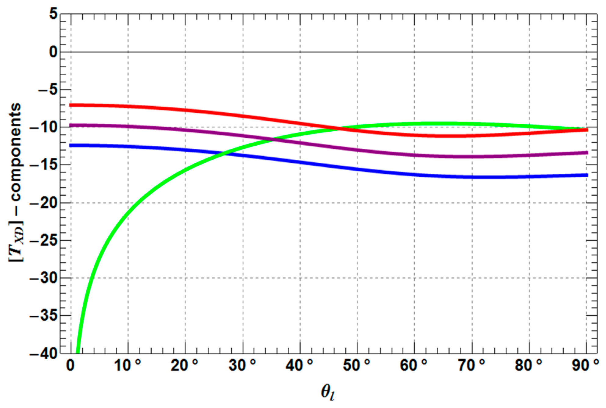
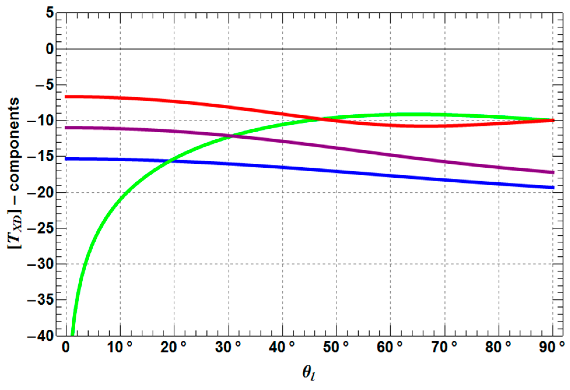
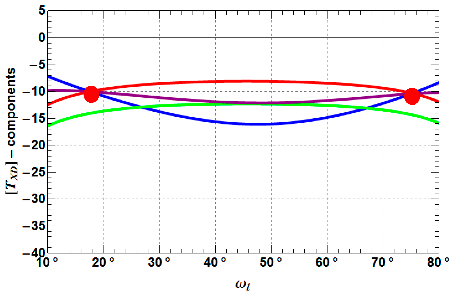
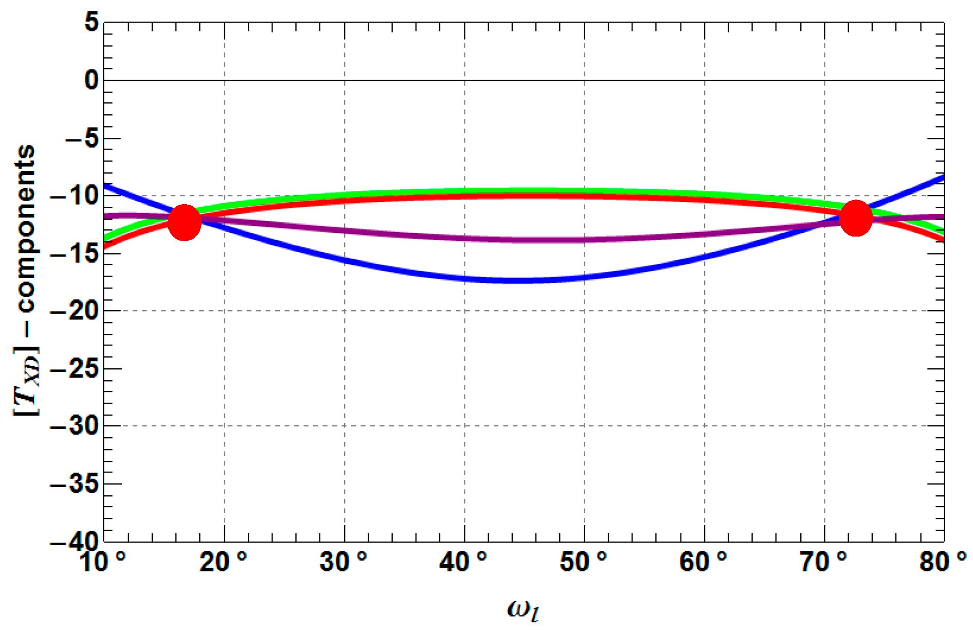
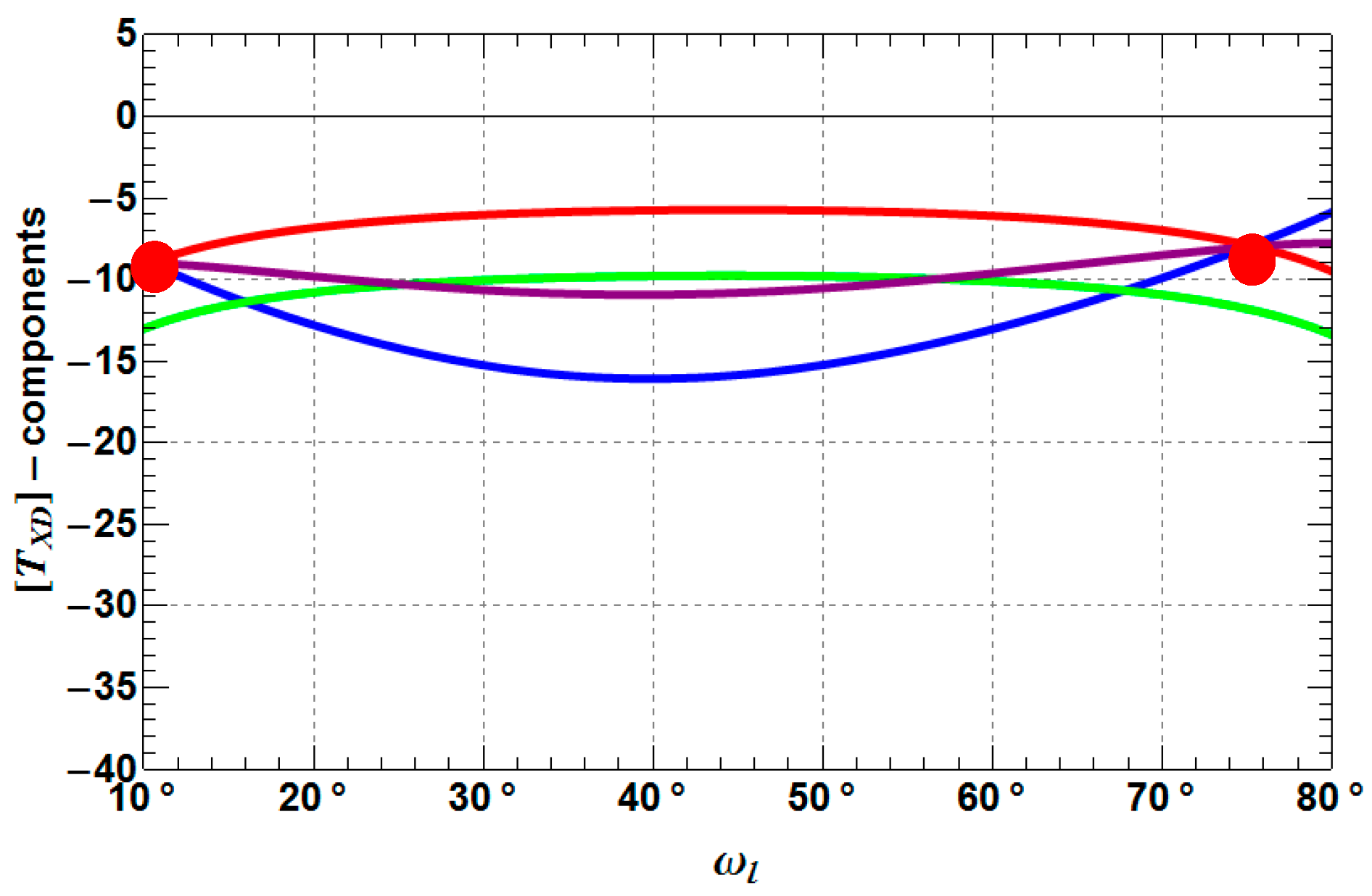
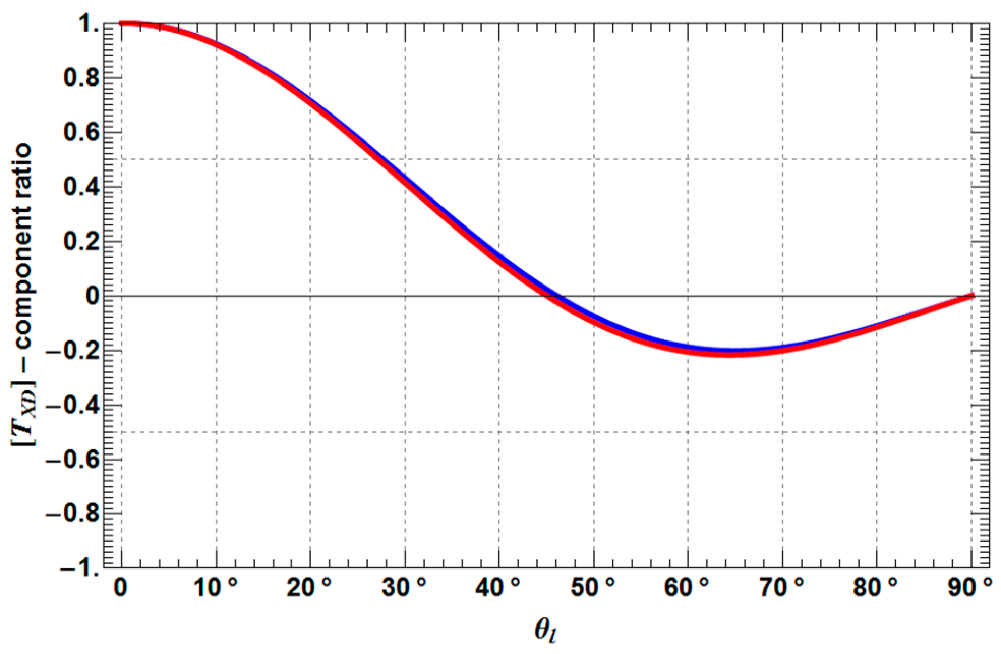
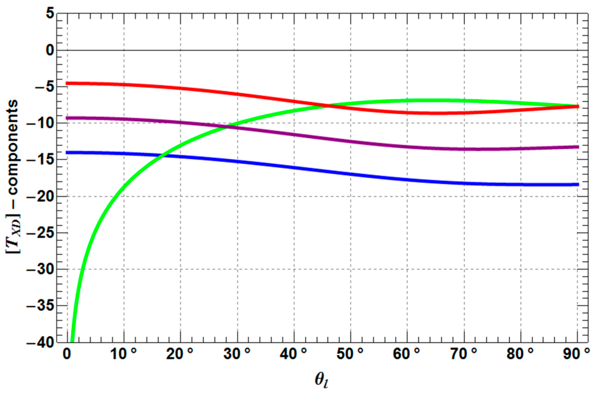
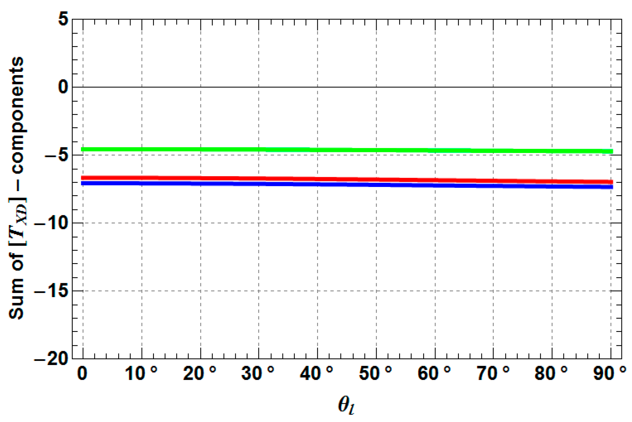
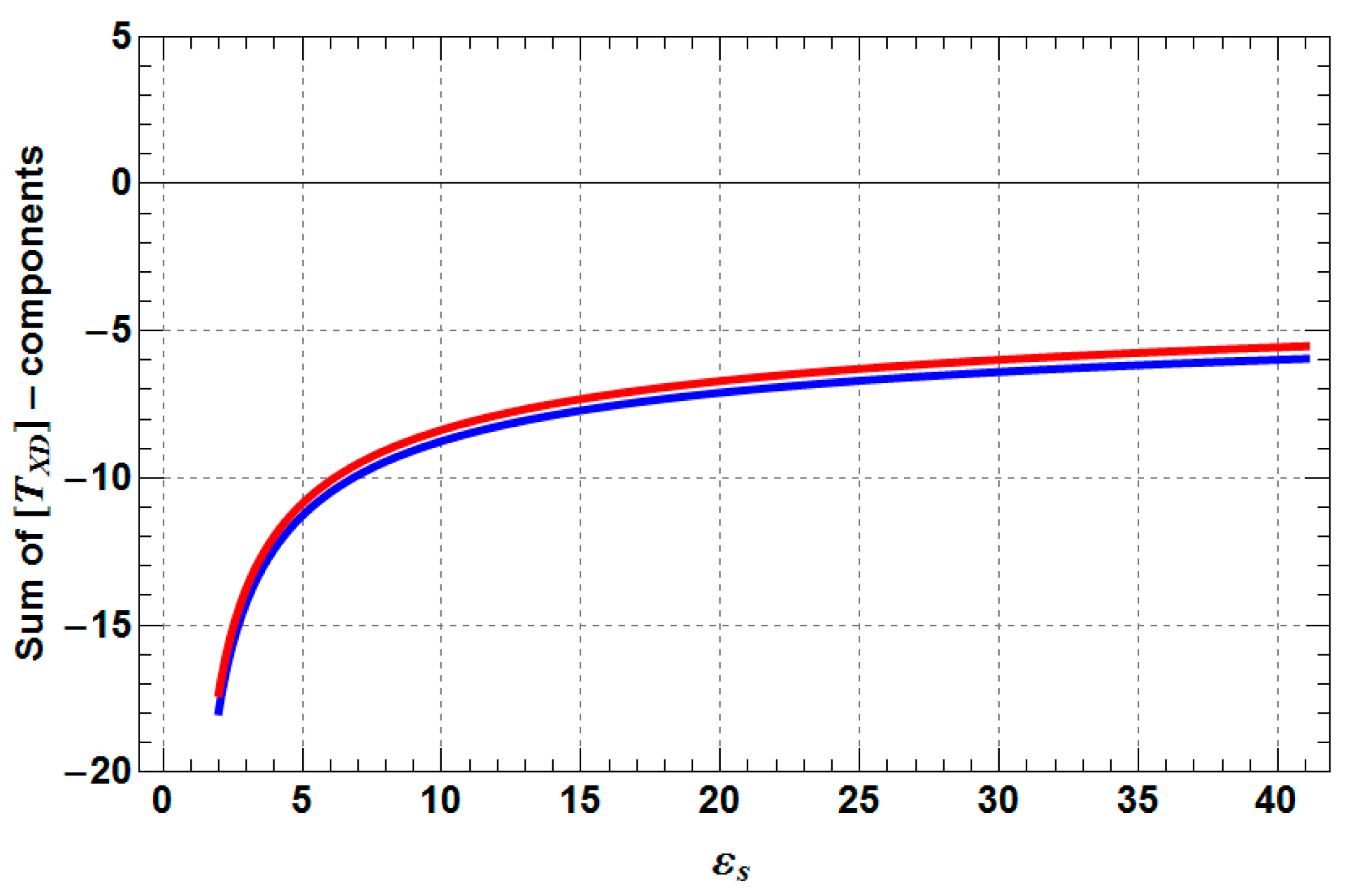
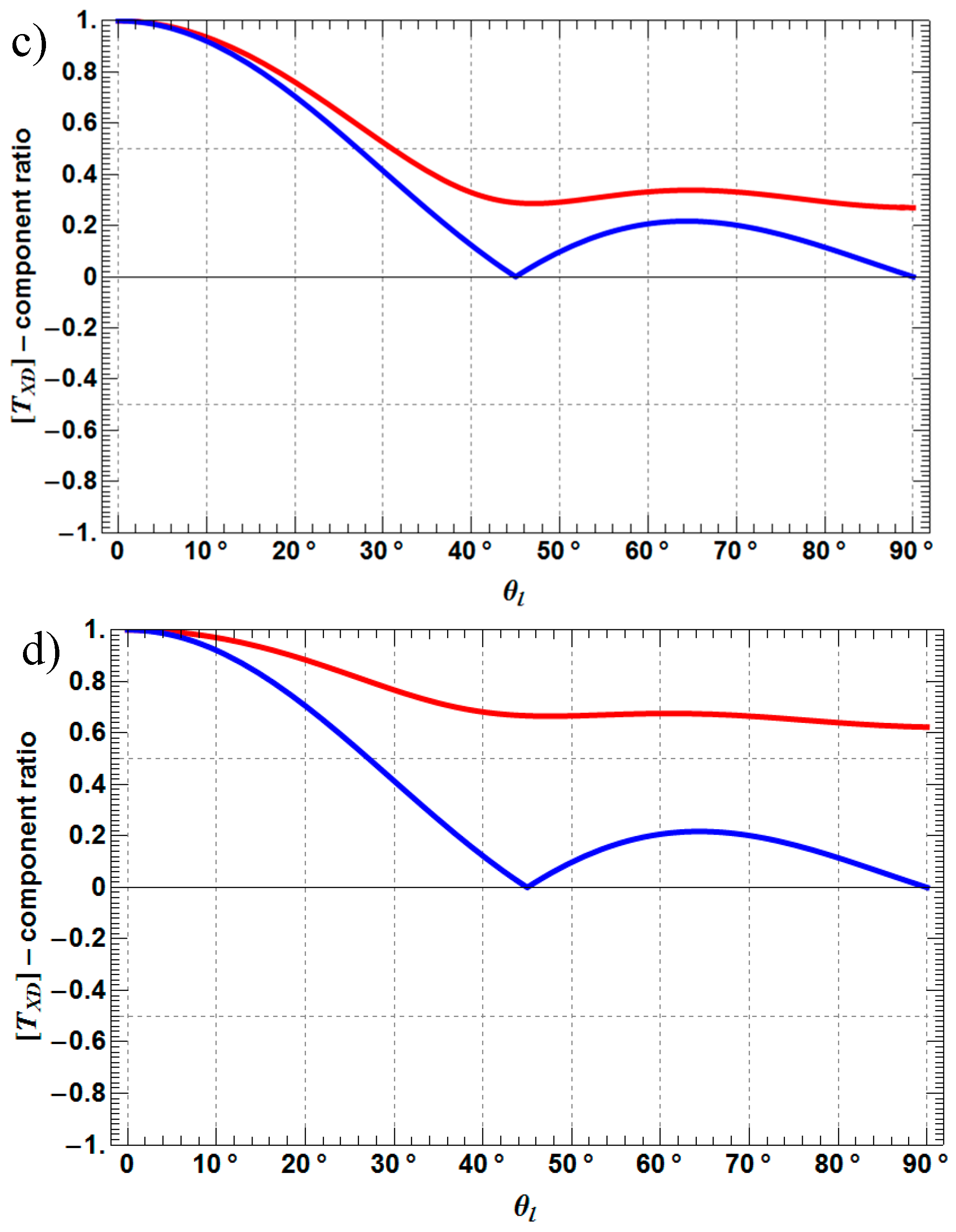
• T_XD11, T_XD12 are decreasing by 3–6 dB with increasing depolarization, while T_XD11 performs as the more stable component of both coherency matrix elements.
• T_XD22 decreases by 3–4 dB with increasing depolarization, but stays always higher than T_XD11, which is a mandatory condition for the presence of dihedral scattering (compared to surface scattering).
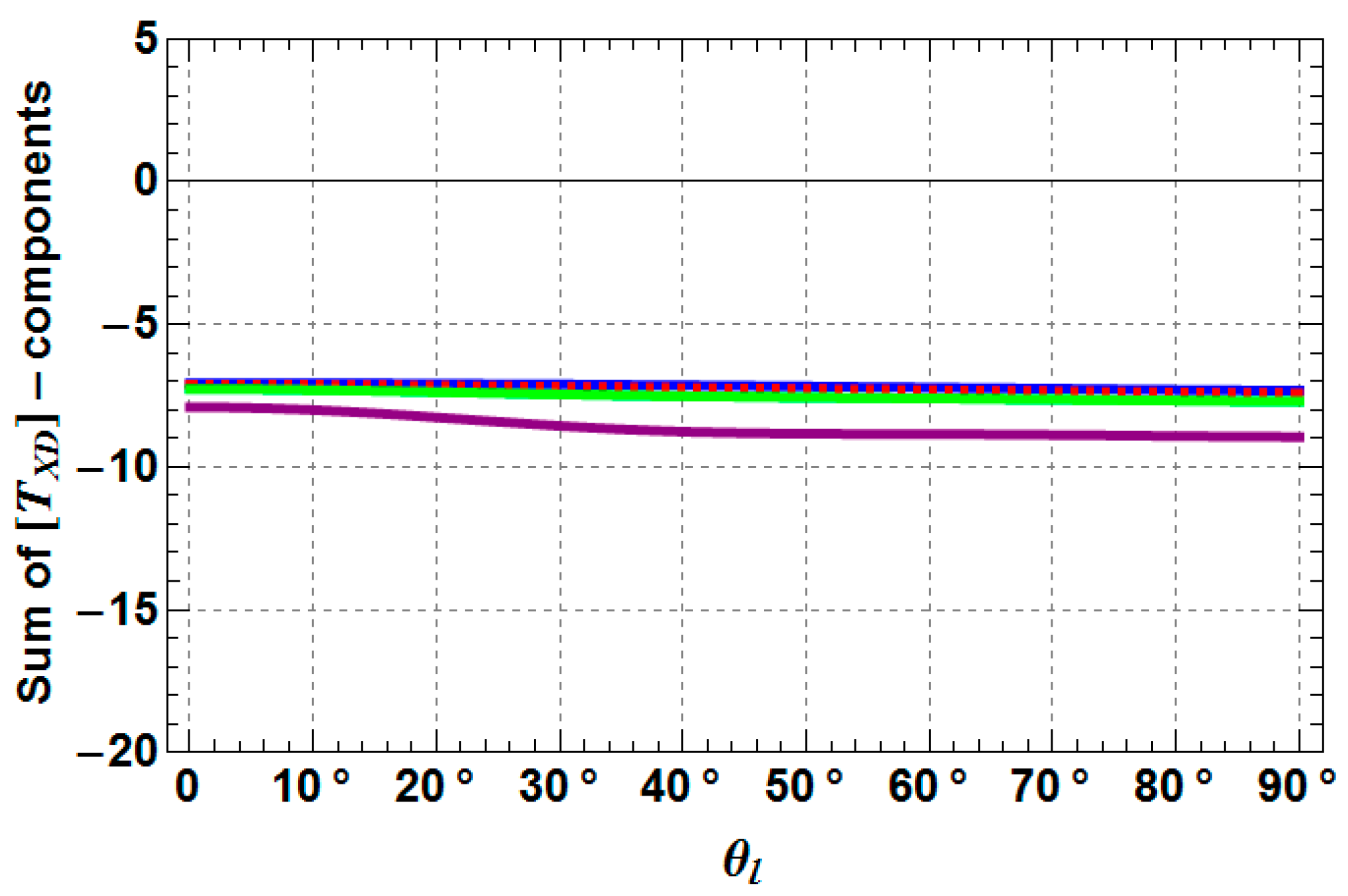
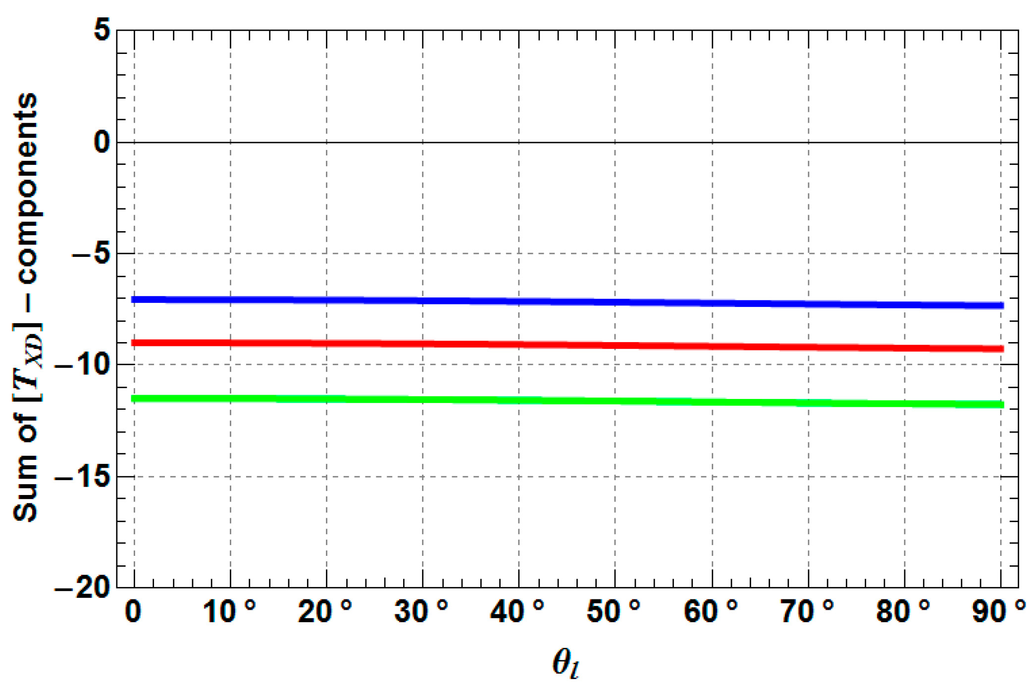
• T_XD33 increases up to −10 dB from a Rank 1 (T_XD33 = 0) to a Rank 3 (T_XD33 > 0) scattering mechanism with increasing depolarization. For weak to medium depolarization (first half of the θ₁-range: 0°–45°) T_XD22 dominates over T_XD33, which reverses for the case of strong depolarization (second half of the θ₁-range: 45°–90°).

Figure 5, Figure 6 and Figure 7 illustrate the behavior of the coherency matrix elements along the local incidence angle (ω_l) for different roughness (θ₁) and moisture conditions of the soil (ε_s) and the trunk (ε_t). However, only the ω_l-range from 25°–70° is analyzed, wherein the majority of remote sensing platforms acquire data for non-mountainous regions. In general, the trend with local incidence angle (ω_l) has a maximum or a minimum at approximately 45° depending on the coherency matrix element. Thus, one rises from 25°–45° and then decreases from 45° down to 70°, or vice versa. The behavior of the single elements can be explained in more detail:

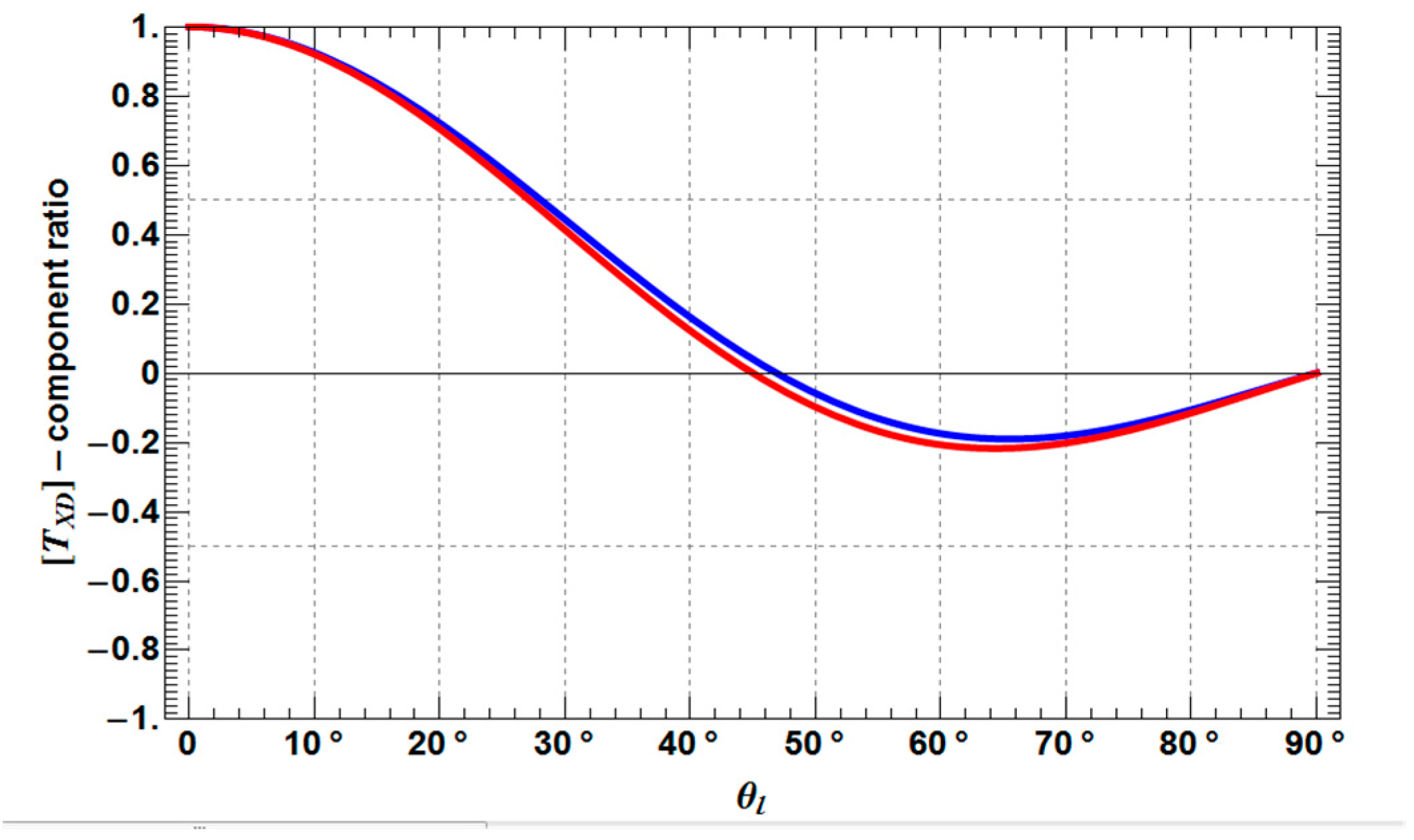
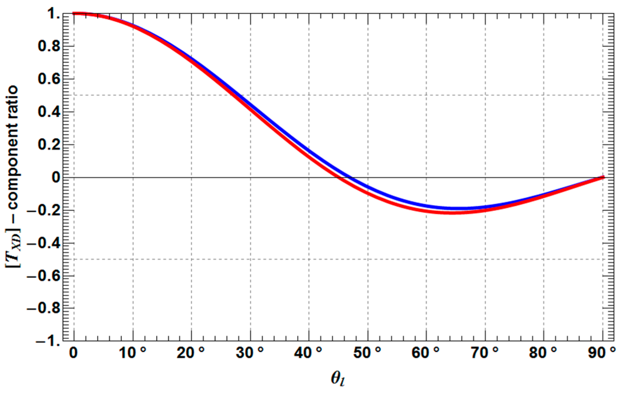
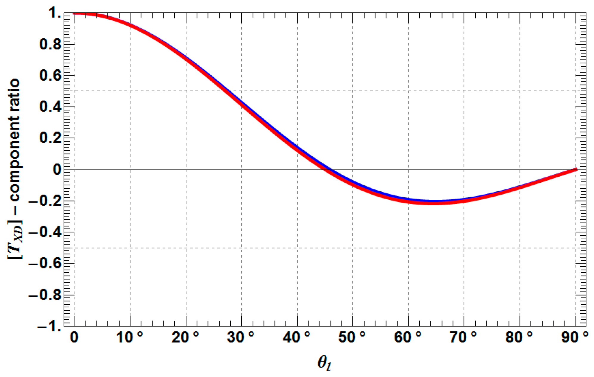
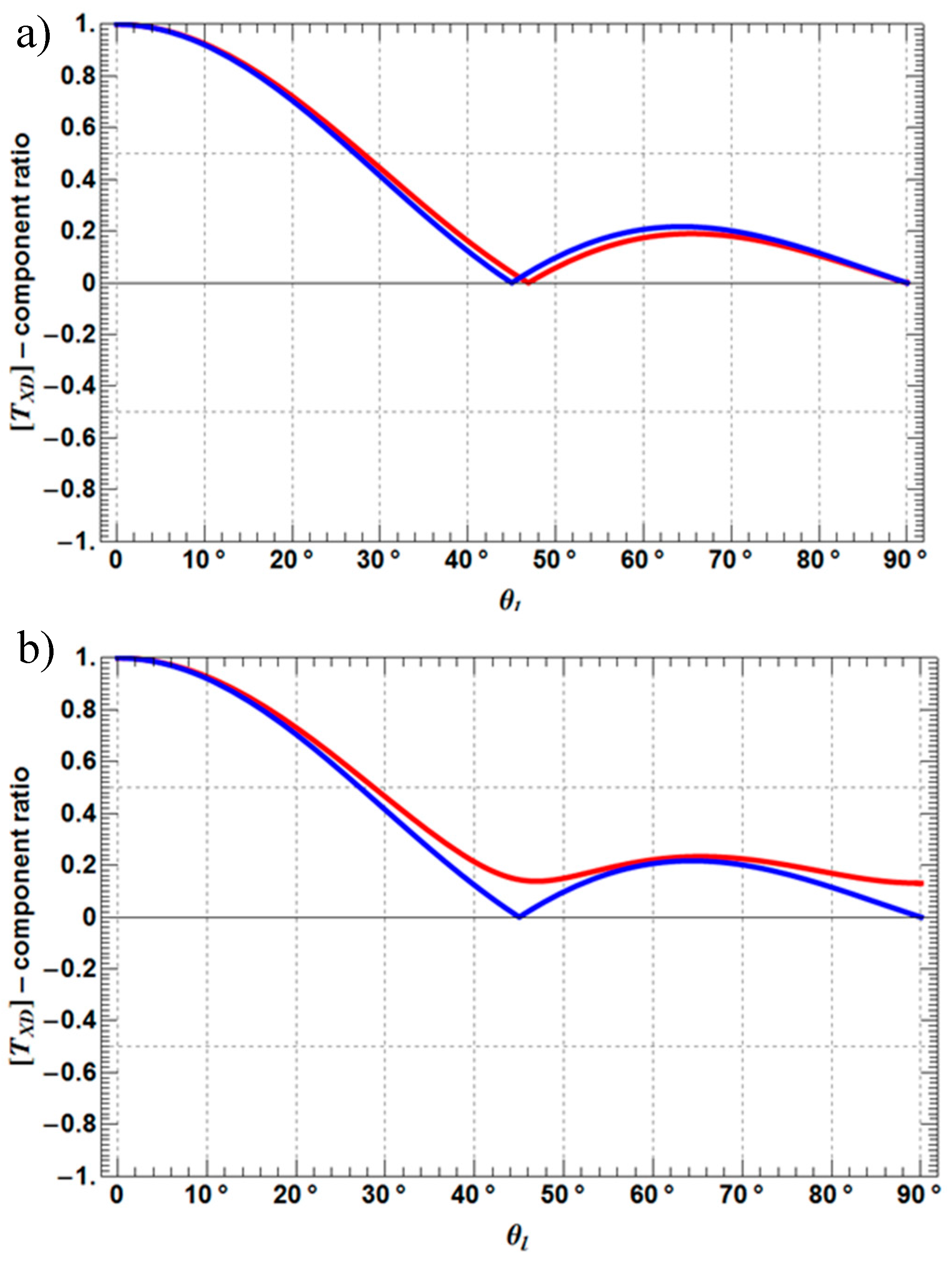
• T_XD11 decreases until approximately 45° and then increase again to the starting level.
• T_XD12 shows the same behavior as T_XD11, but less pronounced.
• T_XD22 and T_XD33 increase until approximately 45° and then decrease to the starting level, while it depends on the roughness depolarization level (θ₁), which curve is superior with respect to the other.
• The crossing points between T_XD11 and T_XD22 represent the Brewster angles of the soil (right crossing) and trunk (left crossing) planes, respectively (see the red points in Figure 5, Figure 6 and Figure 7). The position of the Brewster angles along incidence is related to the soil and trunk dielectric constants. For example, Watanabe et al. analyzed the angular position of the Brewster angles for the potential to retrieve moisture of the soil and the trunks in forested areas [23]. This is an alternative multi-angular method for moisture retrieval, which directly depends on the distinct change of the co-polar phase in dihedral scattering along incidence. The more the covering vegetation canopy is changing the polarization of the penetrating EM waves, the less significant is the phase change and the more biased is the localization of the Brewster angles.

In addition, Figure 8, Figure 9, Figure 10, Figure 11, Figure 12 and Figure 13 depict the behavior of the polarimetric entropy H and the mean scattering alpha angle α with different soil and trunk dielectric contents (ε_s, ε_t), as well as the local incidence ω_l and the roughness depolarization angle θ₁. The polarimetric entropy H is a measure for the degree of disorder in scattering leading to depolarization, while the mean scattering alpha angle α, ranging from 0–π/2, represents an intrinsic scattering type. Both parameters (H, α) stem from an Eigen-based decomposition of the coherency matrix [T_XD] [8].

$$\left[T_{XD}\right]={\lambda }_1\cdot e_1\cdot e_1^{T*}+{\lambda }_2\cdot e_2\cdot e_2^{T*}+{\lambda }_3\cdot e_3\cdot e_3^{T*}$$

(22)

where the coherency-matrix [T_XD] is decomposed into its eigenvalues λ and normalized eigenvectors e, in which T* denotes the transpose conjugate. Together with the pseudo-probabilities P and n = 3 (for monostatic systems), the polarimetric entropy H and the mean scattering alpha angle α are formed [8]:

$$P_i={\lambda }_i/{\displaystyle \sum _{j=1}^n{\lambda }_j}$$

(23)

$$H=-{\displaystyle \sum _{i=1}^n{P}_i\cdot {\log }_3{P}_i}$$

(24)

$$\alpha ={\displaystyle \sum _{i=1}^n{P}_i\cdot \mathrm{acos}\left(\left|e_{i1}\right|\right),}{e}_i={\left[\begin{array}{ccc}{e}_{i1}& e_{i2}& e_{i3}\end{array}\right]}^T$$

(25)

The derivation of both Eigen-based parameters (H, α), as well as their physical meaning are explained thoroughly in [8].

The polarimetric entropy, which is closely linked to the roughness-induced depolarization [24], increases significantly with θ₁, as shown by Figure 8 and Figure 9. While, Figure 10 in comparison with Figure 8 states that an increase of the dielectric constants (ε_s, ε_t) does not lead to a distinct increase in polarimetric entropy, which is driven by θ₁. Therefore, both plots exhibit approximately the same entropy-level of H = 0.5. Moreover, the mean scattering alpha angle α, displayed in Figure 11, Figure 12 and Figure 13, ranges always above 60° between local incidence angles of 20°–70°, which is the most common angle range for agricultural SAR monitoring. As known from polarimetric scattering theory, this behavior of α is expected for dihedral dominant scattering, which should always range higher than 60° stating anisotropic to isotropic dihedral scattering (α → 90°) [25]. Finally, Figure 14 and Figure 15 present the polarimetric H – α scattering plane for a medium local incidence angle (ω_l = 35°), revealing the sensitivity of H and α concerning roughness-induced depolarization θ₁ and the dielectric content of both scattering planes (ε_s, ε_t). The dynamics are indicated by black arrows within the figures. The increase in entropy H with θ₁ is clearly visible for both cases and expected, because an increase in roughness/depolarization is clearly linked with a rise in disorder/entropy.

However, the dynamics concerning the mean scattering alpha angle are related to the variation in the trunk ε_t, as well as the soil ε_s dielectric constant, indicating a similar trend (see black arrows in Figure 14 and Figure 15) for both parameters within the scattering planes. Therefore, the discrimination and inversion of soil and trunk moisture cannot be conducted unambiguously within the polarimetric H − α scattering plane, as changes of both moistures trigger similar patterns within the plane. In addition, for entropies higher than 0.6, the different realizations are localized in a dense grid, and an unambiguous inversion becomes impossible. This is a major difference to the X-Bragg model, where an LoS-rotation-invariant inversion of soil moisture and roughness/depolarization in the H − α plane was feasible straightaway [24]. A variety of combinations of coherency matrix elements were tested with respect to their independence on roughness-induced depolarization or on dielectric properties of the reflecting media for future inversion purposes. The coherency matrix combination T_XD22 + T_XD33 is investigated with its dependencies on ω_l, θ₁, ε_t and ε_s in Figure 16, Figure 17 and Figure 18. Concentrating on Figure 16, the combination T_XD22 + T_XD33 exhibits almost no sensitivity with respect to the roughness-induced depolarization, even for different values of ω_l, ε_t and ε_s. This indicates quasi-independence on roughness-induced depolarization. In addition, Figure 17 and Figure 18 present a strong dependency on the dielectric constant of the soil (ε_s) and the dielectric constant of the trunk (ε_t). Here, the sensitivity is strongest for the lower range of dielectric constants from two to approximately 25. Therefore the combination of coherency matrix elements T_XD22 + T_XD33 seems to be an appropriate candidate to study the dielectric properties of the reflecting media without influence from roughness-induced depolarization.

In contrast, Figure 19, Figure 20, Figure 21 and Figure 22 show the combination of coherency matrix elements (T_XD22 − T_XD33)/(T_XD22 + T_XD33) with respect to the roughness-induced depolarization (θ₁). Since also the function sinc(4θ₁) is plotted as a reference in Figure 19, Figure 20, Figure 21 and Figure 22, the overlap of the two curves for the different ranges of ω_l and of dielectric constants (ε_s, ε_t) is clearly visible. Hence, this combination of coherency matrix elements is only depending on the roughness-induced depolarization and not on the dielectric properties of the media. Moreover, the trend with soil roughness depolarization (θ₁) can be modeled by a simple sinc-function and is equivalent to the behavior of the circular coherence magnitude (for reflection symmetric scattering) [12,24]. However, in the case of an inversion for soil roughness depolarization (θ₁), ambiguities occur for strongly depolarizing scenarios with θ₁ > 63°.

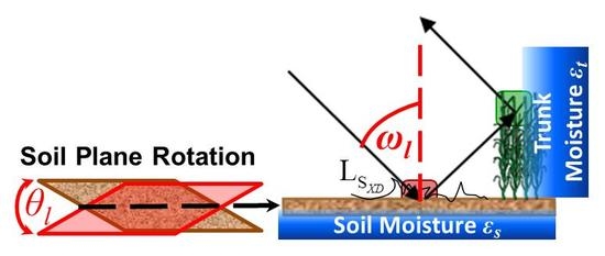
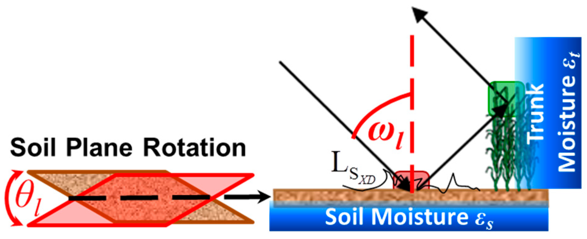
Impact of Differential Phase ϕ and Scattering Loss L_SXD on Coherency Matrix Combinations

As seen in Equation (13), the differential phase ϕ between the two co-polarizations (HH, VV) accounts for the propagation phase difference occurring during the pass through the vegetation volume. Vegetation effects due to preferential orientations have an individual influence on the different polarizations. In Figure 23 and Figure 24, the effect of an increased propagation difference affecting the two co-polarizations is shown for the two T‑matrix combinations T_XD22 + T_XD33 and (T_XD22 − T_XD33)/(T_XD22 + T_XD33). The influence of ϕ on T_XD22 + T_XD33 for phase differences of up to 30° stays below 1 dB of change in power for all roughness levels (0 < ks < 1), which are conventionally occurring due to soil cultivation. Therefore, the differential phase indicates a low impact on this coherency matrix combination. Figure 24 indicates the influence of ϕ on |(T_XD22 − T_XD33)/(T_XD22 + T_XD33)| for phase differences of up to ϕ = 60°. With increasing ϕ the dynamic range of |(T_XD22 − T_XD33)/(T_XD22 + T_XD33)| decreases, and the sensitivity to higher roughness levels (θ₁ > 45°) declines strongly until a complete loss of sensitivity in the range of θ₁ > 40° for a ϕ-level of 30°. Focusing on the impact of the scattering loss L_SXD, the coherency matrix combination T_XD22 + T_XD33 is directly depending on the loss level reducing its power from −7 dB down to −11.5 dB with decreasing of L_SXD from 1.0 (no loss) to 0.6 (60%), as indicated in Figure 25. Fortunately, the matrix combination (T_XD22 − T_XD33)/(T_XD22 + T_XD33) is a ratio, canceling the L_SXD-factor, and is therefore independent from the influences caused by scattering losses.

4. Investigation of Experimental SAR Data for Extended Fresnel Scattering in Agriculture

A rough dihedral scattering component, exhibiting extended Fresnel (X-Fresnel) scattering, requires a distinct vertically-oriented scattering medium, e.g., plant stalks, as well as a horizontal scattering medium with a rough surface, like for instance, a rough soil surface created by agricultural field cultivation.

In order to study extended Fresnel scattering, fully polarimetric SAR data at the L-band of the AgriSAR [26], OPAQUE [27], SARTEO [28] and TERENO [29] project campaigns, including a big variety of crop types in different phenological stages were used. Initially, the data were acquired by DLR’s E-SAR and F-SAR sensor for polarimetric scattering analyses over several agricultural sites [26,27,28,29]. L-band was selected as the appropriate wavelength for the investigation of X-Fresnel scattering due to its higher penetration capability into agricultural vegetation compared to shorter wavelength (X- and C-band) and due to its sufficient signal-to-noise ratio compared to even longer wavelengths, like P-band. Winter crop fields, like for instance winter wheat or winter barley, and farming grassland, which have a distinct stalk component in May, June and July exhibiting potentially X-Fresnel scattering, are investigated for their scattering behavior.

In order to compare the model with data, the scattering mechanism parameter α_XD is calculated from the model (see Equation (17)) and from the L-band SAR data:

$${\alpha }_{XD}^{Data}=\left|T_{12}\right|/T_{22}$$

(26)

Figure 26 shows the modeled α_XD from the X-Fresnel scattering model with the variation of the roughness depolarization angle θ₁ for different values of local incidence angle ω_l assuming a medium moisture scenario (ε_s = 25, ε_t = 15). The analysis indicates that α_XD from the X-Fresnel model generally decreases until about 50° local incidence and then strongly rises until ω_l = 70°. This increase is especially strong for roughness angles around 50°. Concerning very rough soils (θ₁ > 70°), the behavior is opposed to the previous case, and α_XD diminishes with respect to increasing local incidence.

Moving to the analysis of α_XD in the data, Figure 27 displays exemplarily the main scattering mechanisms indicated by the normalized scattering components of the Pauli decomposition for two campaigns (AgriSAR 2006, OPAQUE 2007). The focus of analysis concerning the different scattering mechanisms is on the red color in Figure 27a–c indicating the even-bounce/dihedral scattering as dominant, which is clearly visible on several agricultural fields. The land use of the AgriSAR and OPAQUE campaigns (Figure 27d,h) states that predominantly winter crops and grassland exhibit dihedral/Fresnel and potentially X-Fresnel scattering as the dominating scattering mechanism compared to surface or volume scattering in May–July.

For a first comparison, the α_XD-parameter is calculated from the OPAQUE and AgriSAR data and presented in Figure 27e–g. Regions with strong surface scattering, which appear blue in Figure 27a–c, exhibit high α_XD-values (α_XD > 1.0) in Figure 27e–g, while regions with distinct dihedral scattering indicate low α_XD-values (α_XD < 0.8). This implies a domination of the correlation term T₁₂ over the even-bounce/dihedral term T₂₂ in the case of surface Bragg scattering compared to dihedral Fresnel scattering and vice versa. In Figure 28, the α_XD-values from the Fresnel scattering model (red dashed line) and from the extended Fresnel (black lines) scattering model are compared with mean of field values from the agricultural regions within the AgriSAR, OPAQUE, SARTEO and TERENO project data [26,27,28,29]. Black lines with varying symbols indicate different roughness (θ₁) (depolarization) cases in Figure 28. The single signs with error bars represent α_XD-values from the different campaigns (AgriSAR: plus = June 2006, triangle up = July 2006; OPAQUE: square = May 2007; SARTEO: diamond = May 2008; TERENO: triangle down = May 2012 at the Bode test site, triangle right = May 2012 at the Demmin test site E-W track, triangle left = May 2012 at the Demmin test site N-S track); and the colors assigned to different stalk-dominated crop types from field grass, winter barley, winter triticale, grassland to winter wheat. Despite the distinct standard deviation (gray bars in Figure 28), quantifying around α_XD = 0.1 for all of the means of field values, the match of the mean of the field values with the validity region, spanned by the modeled α_XD-curves for different soil roughness scenarios, is clearly recognizable. While, for instance, the winter barley field (yellow color in Figure 28) seems to be more or less close to the red dashed line, revealing more Fresnel scattering, especially the field grass and winter triticale fields (orchid and green color in Figure 28) appear far from the Fresnel scattering line, showing extended Fresnel scattering with a distinct soil roughness component.

The different plots within Figure 28 reveal the dynamics of the modelled scattering mechanism α_XD with local incidence angle ω_l for different dielectric constants of the soil and the stalks (ε_s, ε_t). While the level of modelled α_XD for low incidence angles (ω_l < 35°) is strongly depending on ε_t (stalks) and minor on ε_s (soil), the situation is reversed for high incidence angles (ω_l > 55°). Therefore, the best modelled α_XD-case is taken in Figure 29 by adjusting the level of ε_s according to available field measurements of soil moisture from the different in situ measurement campaigns. A mean ε_s-level of 10 was found as the most representative approximated dielectric constant value of the soil concerning all campaigns (see Table 1). Unfortunately, only sparse measurements on the vegetation water content were conducted during the field campaigns. Thus, a meaningful and representative ε_t-level from field measurements could not be derived for modelling of the X-Fresnel scattering mechanism α_XD. However, the area of modelled α_XD-values (using the ε_s-level from the measurements) in Figure 29 contains most of the data-derived α_XD-values compared to the non-adapted modelling cases (see Figure 28). This trend is important to signify the logic correctness of the model, as input of in situ conditions during modelling should improve the modelled α_XD-predictions. In Figure 28, more α_XD-values from the data are located outside the modelled α_XD-curves. This again strengthens the indication that the extended Fresnel formalism might be an appropriate model to explain the occurring scattering mechanism in agriculture. However, the analyses just reveal first insights into a potential extended Fresnel scattering mechanism present at L-band for certain crop types in agriculture. Especially the mismatch of the black, modelled curves compared to the extent of the gray bars, representing the standard deviation of the SAR-derived α_XD-values for each of the agricultural fields, in Figure 28 and Figure 29, indicates that by far, not all double-bounce scattering scenarios in agriculture can be represented by a depolarizing double-bounce mechanism using extended Fresnel scattering, as it still represents a significantly simplified scattering scenario.

5. Discussion on Potentials and Limitations

Section 3 and Section 4 introduced an extended Fresnel scattering model and first analysis of the existence of this scattering mechanism in fully-polarimetric, longer wavelength (L-band) SAR data. Shorter wavelengths (X- and C-band) were not analyzed due to their reduced penetration depth in stalk-dominated, maturing winter crops, unlikely to induce a double Fresnel reflection (rough-soil to plant stalks). Hence, the model is only qualified for lower frequency analysis of properties, like soil conditions (roughness, moisture) in agriculture.

The sensitivity analysis of the model on soil roughness-induced depolarization and dielectric properties of the media revealed the dependencies of the coherency matrix elements. The two coherency matrix combinations T_XD22 + T_XD33 and (T_XD22 − T_XD33)/(T_XD22 + T_XD33) showed special sensitivities concerning only soil roughness-induced depolarization or concerning only the dielectric properties of the reflecting media.

While T_XD22 + T_XD33 appears solely dependent on the dielectric properties and not on roughness-induced depolarization, (T_XD22 − T_XD33)/(T_XD22 + T_XD33) has reversed sensitivities. However, it is important to note that the combination (T_XD22 − T_XD33)/(T_XD22 + T_XD33) is also free from the roughness scattering loss factor (L_SXD), whereas the combination T_XD22 + T_XD33 is still depending on this factor (see Figure 25). Hence, the L_SXD-dependence of T_XD22 + T_XD33 requires an exact modelling of the intensity of this component, compared to L_SXD-independent ratios, like α_XD and (T_XD22 − T_XD33)/(T_XD22 + T_XD33). However, the exact formulation of the L_SXD-factor is complicated to elaborate rigorously in the case of a depolarizing ground plane with dependence on the angle θ_l. Therefore, the proposed model for extended Fresnel scattering can be mainly utilized to understand a depolarizing dihedral scattering mechanism and its ratio terms (e.g., α_XD and (T_XD22 − T_XD33)/(T_XD22 + T_XD33)). The model serves to a minor extent for obtaining predictions about absolute backscattering intensities of depolarizing dihedral scattering.

In addition to the loss influence, the combinations of coherency matrix elements, (T_XD22 − T_XD33)/(T_XD22 + T_XD33) and T_XD22 + T_XD33, depend on the differential phase angle (ϕ), which was investigated theoretically for its influence in Figure 23 and Figure 24. This sensitivity study revealed that T_XD22 + T_XD33 is quasi-insensitive of differential extinction up to ϕ = 30°, whereas (T_XD22 − T_XD33)/(T_XD22 + T_XD33) correlates clearly with the change of ϕ. For scattering scenarios of strongly polarizing, meaning strongly-oriented media (ϕ > 30°), the contribution of the differential phase can hardly be neglected. Future analysis for the dependency on ϕ with experimental SAR data should provide deeper insight into this relation and the impact, as well as the level of ϕ in real agricultural SAR data. It is anticipated, that in the case of inversion, the retrieval of soil parameters will be constrained until impossible in media causing high (ϕ > 30°) to very high (ϕ > 60°) differential phases.

However, in Section 4, the analyses with E-SAR and F-SAR L-band data over agricultural regions reveal first insights into the extended Fresnel scattering mechanism, occurring only on different winter crops (winter wheat/barley/triticale and winter rape) and grassland fields for the AgriSAR, OPAQUE, SARTEO and TERENO project campaigns. As indicated by Figure 28, several agricultural fields with different crop types can only be modeled with the extended Fresnel (black lines in Figure 28 and Figure 29) instead of the Fresnel scattering mechanism (red dashed line in Figure 28 and Figure 29). Nevertheless, the data analysis based on these selected fields just represents a first approach to X-Fresnel scattering, whose occurrence is confirmed, but will be investigated in more detail within upcoming agricultural SAR campaigns. Especially the lack of soil roughness and plant moisture measurements for the analyzed vegetated winter crop fields hampers a more detailed analysis of the potential to invert for instance soil roughness. Moreover, in situ measurements of soil roughness will lead to a clear distinguishing of which scattering type should be used for modelling the scattering at the soil plane: Bragg or Fresnel scattering. At the moment, Fresnel scattering is applied assuming rough (tilled) soils in agriculture.

Nonetheless, it can be already anticipated from the model analysis in Section 3 that in the case of inversion for soil roughness and soil moisture, constraints exist using the respective coherency matrix elements. For the inversion of surface roughness with (T_XD22 − T_XD33)/(T_XD22 + T_XD33), ambiguities occur for high to very high roughness ranges, where θ₁ is bigger than 63° (ks = 0.7). Therefore very high roughness conditions cannot be inverted unambiguously. This might be of minor concern in agriculture, when dihedral scattering is present. Then, the fields are normally vegetated by crops, and the soil was prepared before for seeding, leading to small roughness conditions (ks $\ll$ 0.7). In contrast, the fields are heavily ploughed at non-vegetated times, but then dihedral scattering should not emerge.

In the end, the data analyses for extended Fresnel scattering imply that this particular scattering case is rather a special type of scattering mechanism in stalk-dominated, agricultural crop fields than a universal type of mechanism leading to wide-area inversion capabilities of soil and plant properties.

6. Summary and First Conclusions

The classical Rank 1 dihedral scattering, often included in model-based decompositions, was extended to account for soil roughness-induced depolarization appearing in the scattering of natural media. Therefore, an azimuthal Line of Sight (LoS) rotation on the soil plane of the double-bounce reflection was used to generate a depolarized dihedral scattering signal after integration over the chosen orientation angle distribution (pdf_θ) and orientation angle width (2θ₁). The results of the sensitivity analysis are shown for the elements of the coherency matrix [T_XD].

It reveals that the combination of coherency matrix elements T_22XD + T_33XD is quasi-independent of the surface roughness-induced depolarization, while the combination (T_22XD − T_33XD)/(T_22XD + T_33XD) is quasi-independent of the dielectric properties of the reflecting media and only depends on the roughness-induced depolarization. Therefore, a depolarization independent retrieval of soil moisture or a direct roughness retrieval from an extended dihedral scattering component might be possible under certain vegetation and soil conditions. The influence of the differential phase should be negligible or stay at least at a low level (ϕ < 15°), and the soil roughness range should range below ks < 0.7 to avoid ambiguities in a later inversion for soil roughness.

Future studies with polarimetric SAR data will investigate the capability of the suggested soil moisture and soil roughness dependencies for inversion purposes from regions with dominant dihedral scattering mechanism in agriculture. Up to now, the first investigations for agricultural fields (showing dominant dihedral scattering) within the AgriSAR, OPAQUE, SARTEO and TERENO project campaigns, detailed in Section 4, already indicate the benefit of modeling the scattering scenario for stalk-dominated winter crops and grassland with an extended Fresnel instead of a classical Fresnel scattering mechanism, since a wider spectrum of α_XD-values can be represented by the novel model, and inversion for geo-physical parameters, like soil moisture or soil roughness, might be enabled under the discussed constraints (see Section 5). This can be also interesting for novel types of polarimetric decompositions using, for instance, multi-angular, polarimetric SAR data, when the dihedral component is non-dominant (unlike in the presented case) and superimposed by volume scattering [30,31].

References

1. JAXA—ALOS-2 Project Team. Advanced Land Observing Satellite -2: DAICHI-2: The Earth Needs a Health Check, Press-Kit Released by Satellite Applications Mission Directorate I of JAXA. Available online: http://global.jaxa.jp/projects/sat/alos2/pdf/daichi2_e.pdf (accessed on 26 September 2016).
2. Rosenqvist, A.; Shimada, M.; Ito, N.; Watanabe, M. ALOS PALSAR: A pathfinder mission for global-scale monitoring of the environment. IEEE Trans. Geosci. Remote Sens. 2007, 45, 3307–3316. [Google Scholar] [CrossRef]
3. Yamaguchi, Y.; Sato, A.; Sato, R.; Yamada, H.; Yang, J. A new four-component scattering power decomposition applied to ALOS-PALSAR PLR data sets. In Proceedings of 8th European Conference on Synthetic Aperture Radar, Aachen, Germany, 7–10 June 2010.
4. Morena, L.V.; James, K.V.; Beck, J. An introduction to the RADARSAT-2 mission. Can. J. Remote Sens. 2004, 30, 221–234. [Google Scholar] [CrossRef]
5. Liu, C.; Shang, J.; Vachon, P.W.; McNairn, H. Multiyear crop monitoring using polarimetric RADARSAT-2 Data. IEEE Trans. Geosci. Remote Sens. 2013, 51, 2227–2240. [Google Scholar] [CrossRef]
6. Krieger, G.; Moreira, A.; Fiedler, H.; Hajnsek, I.; Werner, M.; Younis, M.; Zink, M. TanDEM-X: A satellite formation for high-resolution SAR interferometry. IEEE Trans. Geosci. Remote Sens. 2007, 45, 3317–3341. [Google Scholar] [CrossRef]
7. Hajnsek, I.; Papathanassiou, K.P.; Busche, T.; Jagdhuber, T.; Kim, J.; Sanjuan Ferrer, M.; Sauer, S.; Villano, M. Fully polarimetric terrasar-X data: Data quality and scientific analysis. In Proceedings of IEEE International Geoscience and Remote Sensing Symposium, Honolulu, HI, USA, 25–30 July 2010.
8. Cloude, S.R. Polarisation: Applications in Remote Sensing; Oxford University Press: Oxford, UK, 2010. [Google Scholar]
9. Lee, J.S.; Pottier, E. Polarimetric. Radar Imaging: from Basics to Applications; Taylor & Francis: Boca Raton, FL, USA, 2009. [Google Scholar]
10. Cloude, S.R.; Pottier, E. A review of target decomposition theorems in radar polarimetry. IEEE Trans. Geosci. Remote Sens. 1996, 34, 498–518. [Google Scholar] [CrossRef]
11. Freeman, A.; Durden, S.L. A three-component scattering model for polarimetric SAR data. IEEE Trans. Geosci. Remote Sens. 1998, 36, 963–973. [Google Scholar] [CrossRef]
12. Jagdhuber, T. Soil Parameter Retrieval under Vegetation Cover Using Sar Polarimetry. Ph.D. Thesis, University of Potsdam, Potsdam, Germany, 2012. [Google Scholar]
13. Yamaguchi, Y.; Yajima, Y.; Yamada, H. A four component decomposition of POLSAR images based on the coherency matrix. IEEE Trans. Geosci. Remote Sens. Lett. 2006, 3, 292–296. [Google Scholar] [CrossRef]
14. Hajnsek, I.; Jagdhuber, T.; Schoen, H.; Papathanassiou, K.P. Potential of estimating soil moisture under vegetation cover by means of PolSAR. IEEE Trans. Geosci. Remote Sens. 2009, 47, 442–454. [Google Scholar] [CrossRef]
15. Ulaby, F.T.; Held, D.; Dobson, M.C.; McDonald, K.C.; Senior, T.B.A. Relating polaization phase difference of sar signals to scene properties. IEEE Trans. Geosci. Remote Sens. 1987, GE-25, 83–92. [Google Scholar] [CrossRef]
16. Lee, B.J.; Khuu, V.P.; Zhang, Z.M. Partially coherent spectral transmittance of dielectric thin films with rough surfaces. J. Thermophys. Heat Transf. 2005, 19, 360–366. [Google Scholar] [CrossRef]
17. Arii, M.; van Zyl, J.J.; Kim, Y. A general characterization for polarimetric scattering from vegetation canopies. IEEE Trans. Geosci. Remote Sens. 2010, 48, 3349–3357. [Google Scholar] [CrossRef]
18. Arii, M.; van Zyl, J.J.; Kim, Y. Improvement of adaptive-model based decomposition with polarization orientation compensation. In Proceedings of IGARSS, Munich, Germany, 22–27 July 2012.
19. Dahon, C.; Ferro-Famil, L.; Titin-Schnaider, C.; Pottier, E. Computing the double-bounce reflection coherent effect in an incoherent electromagnetic scattering model. IEEE Trans. Geosci. Remote Sens. Lett. 2006, 3, 241–245. [Google Scholar] [CrossRef]
20. Lee, J.S.; Ainsworth, T.L.; Wang, Y. Generalized polarimetric model-based decomposition using incoherent scattering models. IEEE Trans. Geosci. Remote Sens. 2014, 52, 2474–2491. [Google Scholar] [CrossRef]
21. Neumann, M. Remote Sensing of Vegetation Using Multi-Baseline Polarimetric Sar Interferometry: Theoretical Modelling and Physical Parameter Retrieval. Ph.D. Thesis, University of Rennes 1, Rennes, France, 2009. [Google Scholar]
22. Al-Kahachi, N. Polarimetric SAR Modelling of a Two-Layer Structure—A Case Study Based on Subartic Lakes. 2014-01; German Aerospace Center: Oberpfaffenhofen, Germany, 2014. [Google Scholar]
23. Watanabe, T.; Yamada, H.; Arii, M.; Park, S.; Yamaguchi, Y. Model experiment of permittivity retrieval method forforested area by using Brewster's angle. In Proceedings of IGARSS, Munich, Germany, 22–27 July 2012.
24. Hajnsek, I.; Pottier, E.; Cloude, S.R. Inversion of surface parameters from polarimetric SAR. IEEE Trans. Geosci. Remote Sens. 2003, 41, 159–164. [Google Scholar] [CrossRef]
25. Cloude, S.R.; Pottier, E.; Boerner, W.M. Unsupervised image classification using the Entropy/Alpha/Anisotropy method in radar polarimetry. In Proceedings of the 2002 AIRSAR Earth Sciences and Applications Workshop; Jet Propulsion Laboratory: Pasadena, CA, USA, 2002. [Google Scholar]
26. Bianchi, R.; Davidson, M.; Hajnsek, I.; Wooding, M.; Wloczyk, C. AgriSAR 2006—Final Report; 19974/06/I-LG; European Space Agency: Paris, France, 2006. [Google Scholar]
27. Jagdhuber, T.; Hajnsek, I. OPAQUE 2007: Kampagnen-und Prozessierungsbericht; DLR-OPAQUE-2007; German Aerospace Center: Oberpfaffenhofen, Germany, 2009. [Google Scholar]
28. Hajnsek, I.; Jagdhuber, T.; Schoen, H. Sarteo-Data Analysis Report; DLR-HR-SARTEO-002; German Aerospace Center, Microwaves and Radar Institute: Oberpaffenhofen, Germany, 2009. [Google Scholar]
29. Jagdhuber, T.; Kohling, M.; Hajnsek, I. TERENO F-SAR Airborne Campaign 2011 @ Rur, Bode and Ammer catchments. In Proceedings of the CT Environmental Sensing Meeting, DLR Oberpfaffenhofen, Germany, 29 November 2011.
30. Jagdhuber, T.; Hajnsek, I.; Papathanassiou, K.P. Soil moisture estimation under vegetation applying polarimetric decomposition techniques. In Proceedings of the 4th International Workshop on Science and Applications of Sar Polarimetry and Polarimetric Interferometry, Frascati, Italy, 26–30 January 2009.
31. Jagdhuber, T.; Hajnsek, I.; Bronstert, A.; Papathanassiou, K.P. Soil moisture estimation under low vegetation cover using a multi-angular polarimetric decomposition. IEEE Trans. Geosci. Remote Sens. 2012, 51, 2201–2215. [Google Scholar] [CrossRef]
Figure 1. Conceptual visualization of the depolarizing soil-trunk double-bounce scattering including the different input variables for extended Fresnel scattering: ωl = local incidence angle, θ1 = rotation limit angle of soil plane, LSXD = roughness intensity loss factor.
Remotesensing 08 00818 g001
Figure 2. Sensitivity of coherency matrix elements TXD11 (blue), TXD12 (purple), TXD22 (red) and TXD33 (green) (dB) with roughness angle θ1s = 20, εt = 10, ωl = 30°, LSXD = 1, ϕ = 0°).
Remotesensing 08 00818 g002
Figure 3. Sensitivity of coherency matrix elements TXD11 (blue), TXD12 (purple), TXD22 (red) and TXD33 (green) (dB) with roughness angle θ1 (εs = 20, εt = 10, ω l = 50°, LSXD = 1, ϕ = 0°).
Remotesensing 08 00818 g003
Figure 4. Sensitivity of coherency matrix elements TXD11 (blue), TXD12 (purple), TXD22 (red) and TXD33 (green) (dB) with roughness angle θ1 (εs = 20, εt = 30, ωl = 30°, LSXD = 1, ϕ = 0°).
Remotesensing 08 00818 g004
Figure 5. Sensitivity of coherency matrix elements TXD11 (blue), TXD12 (purple), TXD22 (red) and TXD33 (green) (dB) with local incidence angle ωl (εs = 20, εt = 10, θ1 = 30°, LSXD = 1, ϕ = 0°). Red points indicate the Brewster angle locations.
Remotesensing 08 00818 g005
Figure 6. Sensitivity of coherency matrix elements TXD11 (blue), TXD12 (purple), TXD22 (red) and TXD33 (green) (dB) with local incidence angle ωl (εs = 20, εt = 10, θ1 = 50°, LSXD = 1, ϕ = 0°). Red points indicate the Brewster angle locations.
Remotesensing 08 00818 g006
Figure 7. Sensitivity of coherency matrix elements TXD11 (blue), TXD12 (purple), TXD22 (red) and TXD33 (green) (dB) with local incidence angle ωl (εs = 20, εt = 30, θ1 = 30°, LSXD = 1, ϕ = 0°). Red points indicate the Brewster angle locations.
Remotesensing 08 00818 g007
Figure 8. Sensitivity of polarimetric entropy H with local incidence angle ω1 (εs = 20, εt = 10, LSXD = 1, ϕ = 0°, θ1 = 30°).
Remotesensing 08 00818 g008
Figure 9. Sensitivity of polarimetric entropy H with local incidence angle ω1 (εs = 20, εt = 10, LSXD = 1, ϕ = 0°, θ1 = 60°).
Remotesensing 08 00818 g009
Figure 10. Sensitivity of polarimetric entropy H with local incidence angle ω1 (εs = 20, εt = 30, LSXD = 1, ϕ = 0°, θ1 = 30°).
Remotesensing 08 00818 g010
Figure 11. Sensitivity of polarimetric mean scattering alpha angle α with local incidence angle ω1 (εs = 20, εt = 10, LSXD = 1, ϕ = 0°, θ1 = 30°).
Remotesensing 08 00818 g011
Figure 12. Sensitivity of polarimetric mean scattering alpha angle α with local incidence angle ω1 (εs = 20, εt = 10, LSXD = 1, ϕ = 0°, θ1 = 60°).
Remotesensing 08 00818 g012
Figure 13. Sensitivity of polarimetric mean scattering alpha angle α with local incidence angle ω1 (εs = 20, εt = 30, LSXD = 1, ϕ = 0°, θ1 = 30°).
Remotesensing 08 00818 g013
Figure 14. Sensitivity of polarimetric Hα scattering plane with roughness angle θ1 (εs = (2,42), εt = 10, LSXD = 1, ϕ = 0°, ω1 = 35°). Color changes with increasing θ1.
Remotesensing 08 00818 g014
Figure 15. Sensitivity of polarimetric Hα scattering plane with roughness angle θ1 (εs = 10, εt = (2,42), LSXD = 1, ϕ = 0°, ω1 = 35°). Color changes with increasing θ1.
Remotesensing 08 00818 g015
Figure 16. Sensitivity of coherency matrix combination TXD22 + TXD33 (blue) (dB) with roughness angle θ1; blue: εs = 20, εt = 10, ωl = 30°; green: εs = 20, εt = 30, ωl = 30°; red: εs = 20, εt = 10, ωl = 50° and LSXD = 1, ϕ = 0°.
Remotesensing 08 00818 g016
Figure 17. Sensitivity of coherency matrix combination TXD22 + TXD33 (blue) (dB) with the dielectric of the soil εs; blue: θ1 = 30°, εt = 10; red: θ1 = 50°, εt = 10 and ωl = 30°, LSXD = 1, ϕ = 0°.
Remotesensing 08 00818 g017
Figure 18. Sensitivity of coherency matrix combination TXD22 + TXD33 (blue) (dB) with the dielectric of the trunk εt (θ1 = 30°, εs = 20, ωl = 30°, LSXD = 1, ϕ = 0°).
Remotesensing 08 00818 g018
Figure 19. Sensitivity of (TXD22TXD33)/(TXD22 + TXD33) with roughness angle θ1 (blue) (εs = 20, εt = 10, ωl = 30°, ϕ = 0°) and comparison with sinc(4θ1) (red).
Remotesensing 08 00818 g019
Figure 20. Sensitivity of (TXD22TXD33)/(TXD22 + TXD33) with roughness angle θ1 (blue) (εs = 20, εt = 10, ωl = 60°, ϕ = 0°) and comparison with sinc(4θ1) (red).
Remotesensing 08 00818 g020
Figure 21. Sensitivity of (TXD22TXD33)/(TXD22 + TXD33) with roughness angle θ1 (blue) (εs = 20, εt = 30, ωl = 30°, ϕ = 0°) and comparison with sinc(4θ1) (red).
Remotesensing 08 00818 g021
Figure 22. Sensitivity of (TXD22TXD33)/(TXD22 + TXD33) with roughness angle θ1 (blue) (εs = 30, εt = 30, ωl = 30°, ϕ = 0°) and comparison with sinc(4θ1) (red).
Remotesensing 08 00818 g022
Figure 23. Sensitivity of TXD22 + TXD33 along roughness angle θ1 (εs = 20, εt = 10, ωl = 30°, LSXD = 1) with differential phase ϕ = 0° (blue), ϕ = 15° (red, dashed), ϕ = 30° (green) and ϕ = 60° (purple).
Remotesensing 08 00818 g023
Figure 24. Sensitivity of |(TXD22 - TXD33)/(TXD22 + TXD33)| along roughness angle θ1 (red) (εs = 20, εt = 10, ωl = 30°, LSXD = 1) with differential phases ϕ = 0° (a), ϕ = 15° (b), ϕ = 30° (c), ϕ = 60° (d) and comparison with |sinc(4θ1)| (blue).
Remotesensing 08 00818 g024aRemotesensing 08 00818 g024b
Figure 25. Sensitivity of TXD22 + TXD33 along roughness angle θ1 (εs = 20, εt = 10, ωl = 30°, ϕ = 0°) with scattering loss LSXD = 1.0 (blue), LSXD = 0.8 (red) and LsXD = 0.6 (green).
Remotesensing 08 00818 g025
Figure 26. Sensitivity of αXD along the roughness angle θ1; αXD is derived from the X-Fresnel scattering model (εs = 25, εt = 15, ϕ = 0°) for different angles of local incidence ωl. Gray dashed arrow indicates dynamics with ωl.
Remotesensing 08 00818 g026
Figure 27. First row: RGB-composite of normalized Pauli decomposition-based scattering components (R: 1/2|SHH − SVV|² even-bounce/dihedral scattering, G: 2|SXX|² volume/vegetation scattering, B: 1/2|SHH + SVV|² odd-bounce/surface scattering) for the May acquisition of the OPAQUE 2007 (a), the June acquisition (b) and the July acquisition (c) of the AgriSAR 2006 campaign; (d) the land use of the AgriSAR 2006 campaign; second row: comparison of αXD of the data for the OPAQUE 2007 campaign (e) and the AgriSAR campaign (f) June acquisition and (g) July acquisition); (h) the land use of the OPAQUE 2007 campaign.
Remotesensing 08 00818 g027
Figure 28. Comparison of αXD from extended Fresnel scattering (black lines) and from standard Fresnel scattering (red dashed line) along the local incidence angle ωl; αXD is derived from the X-Fresnel model (εs = 25, εt = 15, ϕ = 0° (a); εs = 15, εt = 25, ϕ = 0° (b); εs = 25, εt = 25; ϕ = 0° (c)) for different roughness angles θ1 and from the AgriSAR (plus (June) and triangle up (July) sign), OPAQUE (square sign), SARTEO (diamond sign) and TERENO (triangle down = Bode site, triangle right Demmin site E-W track, triangle left Demmin site N-S track) L-band data for several agricultural fields with a stalk-dominated phenology (yellow = winter barley, green = field grass, gold = winter wheat, pink = winter wheat (field 221), cyan = grassland, red = undefined land use, orchid = winter triticale); gray bars indicate the standard deviation of αXD for each of the agricultural fields.
Remotesensing 08 00818 g028
Figure 29. Comparison of αXD from extended Fresnel scattering (black lines) and from standard Fresnel scattering (red dashed line) along the local incidence angle ωl; αXD is derived from the X-Fresnel model with εs-input from local field measurements (εs = 10, εt = 25, ϕ = 0°) for different roughness angles θ1 and from the AgriSAR (plus (June) and triangle up (July) sign), OPAQUE (square sign), SARTEO (diamond sign) and TERENO (triangle down = Bode site, triangle right Demmin site E-W track, triangle left Demmin site N-S track) L-band data for several agricultural fields with a stalk-dominated phenology (yellow = winter barley, green = field grass, gold = winter wheat, pink = winter wheat (field 221), cyan = grassland, red = undefined land use, orchid = winter triticale); gray bars indicate the standard deviation of αXD for each of the agricultural fields.
Remotesensing 08 00818 g029