Article

A Quantitative Comparison of Total Suspended Sediment Algorithms: A Case Study of the Last Decade for MODIS and Landsat-Based Sensors

Remote Sensing and Satellite Research Group, Curtin University, GPO Box U1987, Perth 6845, Australia
*
Author to whom correspondence should be addressed.
Remote Sens. 2016, 8(10), 810; https://doi.org/10.3390/rs8100810
Submission received: 2 June 2016 / Revised: 14 September 2016 / Accepted: 24 September 2016 / Published: 30 September 2016

Abstract

:
A quantitative comparative study was performed to assess the relative applicability of Total Suspended Solids (TSS) models published in the last decade for the Moderate Resolution Imaging Spectroradiometer (MODIS) and Landsat-based sensors. The quantitative comparison was performed using a suite of statistical tests and HydroLight simulated data for waters ranging from clear open ocean case-1 to turbid coastal case-2 waters. The quantitative comparison shows that there are clearly some high performing TSS models that can potentially be applied in mapping TSS concentration for regions of uncertain water type. The highest performing TSS models tested were robust enough to retrieve TSS from different water types with Mean Absolute Relative Errors (MARE) of 69.96%–481.82% for HydroLight simulated data. The models were also compared in regional waters of northern Western Australia where the highest performing TSS models yielded a MARE in the range of 43.11%–102.59%. The range of Smallest Relative Error (SRE) and Largest Relative Error (LRE) between the highest and the lowest performing TSS models spanned three orders of magnitude, suggesting users must be cautious in selecting appropriate models for unknown water types.

Graphical Abstract

1. Introduction

The health of coastal waters not only determines the health of marine habitats in the region but also signifies the health of the nearby human inhabitants with nearly 60% of the earth’s population settled in the coastal zones of our oceans and seas, and over 90% of the world’s fish caught for consumption being sourced from coastal waters [1]. The health of water systems is typically determined from a key indicator, the water clarity (turbidity) which is influenced by the amount of dissolved matter and total suspended solids (TSS) comprising organic matter such as algae and other micro-organisms and inorganic particulate matter from minerals [2]. Monitoring TSS along with other water quality parameters is crucial for coastal ecology because TSS can directly affect the turbidity and color of water [3] and turbidity determines the amount of light availability at depth for primary production [4,5,6].
Monitoring the temporal and spatial distribution of TSS in the coastal environment can be a huge undertaking and nearly impossible in terms of financial and time resources if performed using traditional in situ water sampling methods [7] unless coupled with satellite-based remote sensing. Since the early space-borne sensors of the 1970s there has been, and continues to be, a great improvement in the spectral, spatial and temporal resolutions [8]. For example, the Landsat-based series of sensors has evolved over the years from three (red, green and blue) spectral bands with spatial resolutions of 185 m and a revisit time of 18 days to the newest Landsat-8 with 11 spectral bands (433–12,500 nm) with spatial resolutions of 30 m (and 15 m panchromatic) and a revisit time of 16 days. The shortcoming of the long revisit time for Landsat can be filled by the readily available MODIS-Aqua and Terra sensors which have shorter revisit times of one day, and with 36 spectral bands (405–14,385 nm) and spatial resolutions from 250 m to 1000 m.
Since the launch of the early remote sensing satellites in the early 1970s many studies have been conducted in remotely mapping TSS, driven in part by the capability of satellite remote sensing to cover large spatial domains in near real time [7]. Considering the past decade, remote sensing studies of the spatial and temporal mapping of TSS have utilized moderate resolution sensors including Landsat [9,10,11,12,13,14,15], MERIS [6,16,17,18,19,20], MODIS [17,21,22,23,24,25,26,27], and high resolution sensors including SPOT [28], IKONOS [29], and THEOS [30]. Further, the TSS mapping studies encompassed waters with diverse optical and physical properties, from inland lakes and river systems [21,25,31,32,33] to coastal waters [34,35,36,37,38] and from different geographical locations including America [3,32,39], Africa [26,40], Asia [16,34,41], Australia [42,43], and Europe [17,23,27,37].
The majority of the models developed in retrieving TSS by remote sensing methods are typically locally tuned to a regional water or waters with similar optical properties. Regional tuning of a TSS model is necessary because of the potentially large variation in the inherent optical properties (IOPs) of the water constituents. The theoretical basis of ocean color remote sensing has shown that sensor-measured reflectance of the water is related to the IOPs of the water—absorption and scattering coefficients. IOPs vary with the types and amounts of the water’s constituents, such as sediments, phytoplankton, detrital matter and CDOM [44] which may be different for different sediment types and phytoplankton types in different regions. In addition, factors such as water depth, viewing geometry, and atmospheric conditions all add to the complexity of the relationship between the measurement of reflectance of the water surface and the IOPs and concentrations of constituents [45].
TSS models are generally classified into three categories, (1) an empirical model where TSS is modelled directly using a statistical analysis to relate the apparent optical properties (AOPs); (2) an analytic model that relates the IOPs and AOPs of water through radiative transfer theory to derive TSS; and (3) a semi-analytic model that is partly based on the empirical analysis and grounded on the radiative transfer theory [7]. Individual TSS model designs have their own limitations and advantages. An empirical model is often sought for its simplicity and explanatory power because unique properties of local waters are tuned to each model, but it may lack general applicability. An analytic model is potentially applicable to other water bodies because it is not dependent on the in situ water constituents, but it requires accurate knowledge of water column properties which is often difficult to acquire. The semi-analytic model has both the limitations and advantages associated with the first two models, and it is generally preferred because it has higher explanatory power and is more convenient than the analytic model [7,8].
In the last decade, various TSS models have been developed [35,37,38,46,47] and applied to their respective regions with a wide range of success with reported retrieval errors ranging from lows of ~18% to highs of ~61%. Considering each model is developed and tuned for a specific region, water type and its associated IOPs, the application or transferability of the models to other regions is limited, and the likely accuracy of the results unknown. Even when an existing TSS model is applied to waters in similar regions it is often first re-calibrated before being applied. The availability of many TSS algorithms for different regions and sensors warrants one to ask if we can use someone else’s algorithm to estimate TSS in regions where we do not have any in situ observations? For the cross applicability of TSS models between different regions the design of a TSS algorithm has to either be based on analytic methods and grounded on theoretical functions of radiative transfer theory, or the waters must be assumed to have similar optical and physical properties. However, considering the vast number of TSS models that have been developed across different geographical regions with different optical and physical properties we can seek to establish the robustness in the applicability of these existing TSS algorithms for different regions.
A recent study by Brewin, et al. [44] developed an objective methodology where comparison of different bio-optical algorithms are quantitatively and qualitatively considered for use in climate studies. Following the methods of Brewin, et al. [44] and their quantitative methodology to rank the algorithms, in this study we objectively compare the performance of TSS algorithms for MODIS and Landsat sensors developed during the last decade using HydroLight simulated data for different water and sediment types. If shown to be robust, these algorithms would provide marine remote sensing scientists and coastal managers some level of confidence in their ability to assess the quality of water with minimal resource for coastal monitoring of optically unexplored waters. Specifically, this study aims to quantitatively assess the applicability of established TSS algorithms to different water types and quantify the variability in retrieving TSS when using off the shelf TSS algorithms for MODIS and Landsat sensors.

2. Materials and Methods

2.1. Dataset

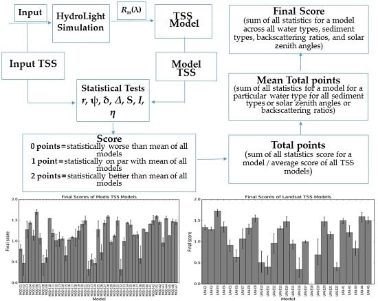
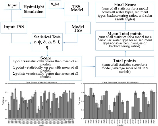
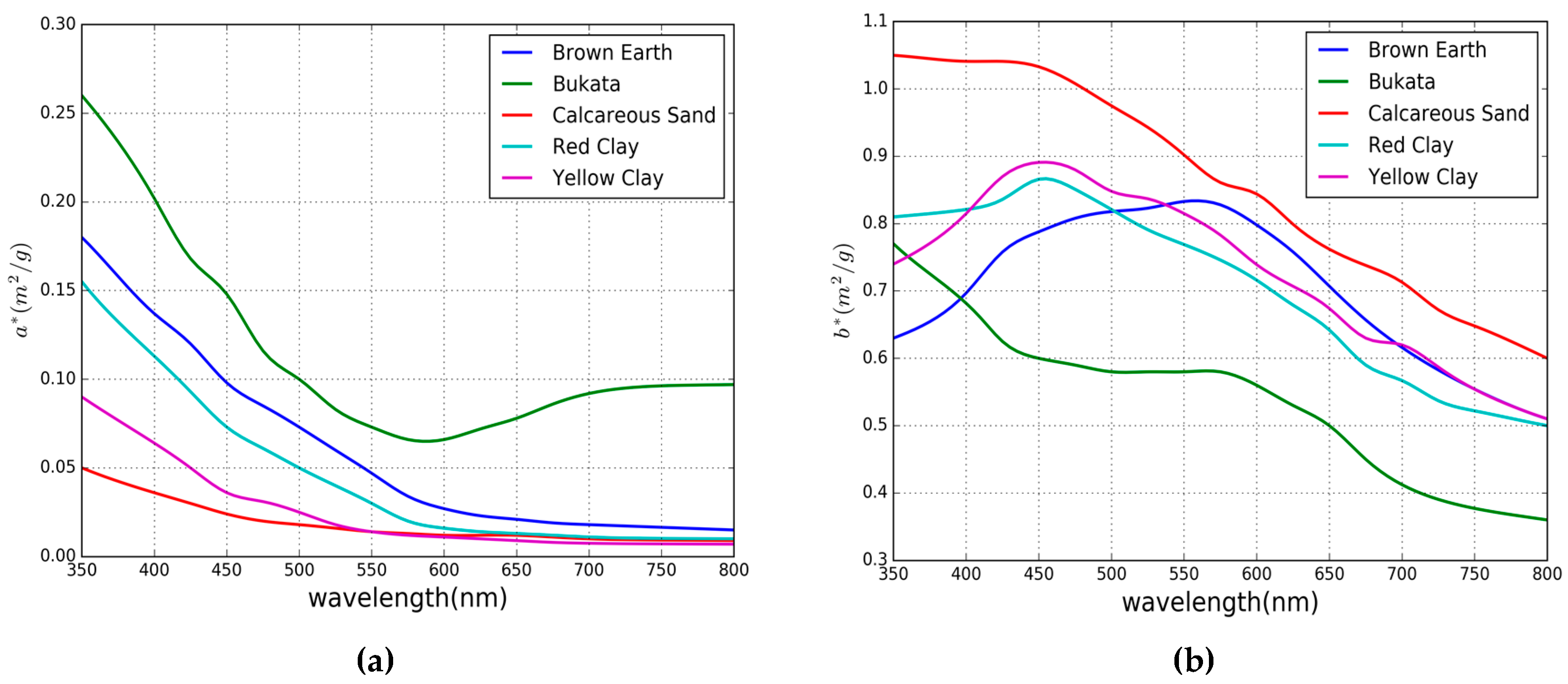
2.1.1. HydroLight Simulation

A set of ocean reflectance spectra were derived using the radiative transfer numerical model HydroLight 4.2 (Sequoia Scientific, Inc., Bellevue, WA 98005, United States of America) in the four component case-2 waters mode. Using a forward model HydroLight solves radiance distributions and derives reflectance and radiance for water bodies with specific inherent optical properties (SIOPs) for given sky and water state conditions [48]. Sub-surface remote sensing reflectance’s (rrs) were computed for infinitely deep water using a range of SIOPs, sea-state, and sky conditions. The spectral range for rrs from HydroLight was simulated for wavelengths (λ) in the range of 400 nm–800 nm at a nominal bandwidth of 4 nm.
For all the HydroLight simulations the sea state was chosen to have a wind speed of 5 m·s−1 and the sky radiance computed using the Harrison and Coombes (1988) normalized radiance model for a clear sky. The diffuse and direct sky irradiances were computed using the Gregg and Carder (1990) irradiance model for a solar zenith angle of 30° [49]. The four components, pure water, chlorophyll (CHL), colored dissolved organic matter (CDOM), and mineral (TSS) were modelled in varying concentrations, presented in Table 1, to be representative of open ocean to turbid coastal waters. For the TSS component, five different sediment types were used, namely (1) brown earth; (2) calcareous sand; (3) yellow clay; (4) red clay; and (5) Bukata from the default database of HydroLight. The phase functions for the components were modelled as Rayleigh like phase function for pure water, Fournier-Forand phase function with bb(λ)/b(λ) of 0.01 for CHL, and Petzold “average particle” phase function for TSS for all the aforementioned HydroLight simulations. In addition to the aforementioned parameters for HydroLight simulations, we further carried out additional simulations using the parameters outlined above but with solar zenith angles of 15°, 30°, 45°, and 60° and bb(λ)/b(λ) ratios of 0.001, 0.01, 0.018, 0.05, and 0.1 for calcareous sand to study the robustness of TSS models to changes in solar angles and the backscattering ratios.
The IOP models used in this HydroLight simulation are described by Equations (1) and (2). The total absorption coefficient (a(λ)) is the sum of absorption coefficients of pure water (aw(λ)), CHL (aϕ(λ)), CDOM (acdom(λ)) and TSS (ap(λ)):
a ( λ ) = a w ( λ ) + a φ ( λ ) + a cdom ( λ ) + a p ( λ )
The total scattering coefficient (b) is the sum of scattering coefficients of pure water (bw(λ)), CHL (bϕ(λ)), and TSS (bp(λ)):
b ( λ ) = b w ( λ ) + b φ ( λ ) + b p ( λ )
The total backscattering coefficient is expressed as the sum of backscattering coefficients for pure sea water (bbw(λ)), particulates (bbp(λ)), and phytoplankton pigments (b(λ)).
b b ( λ ) = b bw ( λ ) + b bp ( λ ) + b b φ ( λ )
The SIOP models allow the scaling of the IOP of each component with concentration (X):
a i ( λ ) = a i * ( λ ) × X i
b i ( λ ) = b i * ( λ ) × X i
where i is the component and ai*(λ) and bi*(λ) are component specific absorption and scattering coefficients.
The SIOP of each component was either obtained from HydroLight’s default dataset or modeled using established models. For the specific absorption and scattering coefficients: the absorption coefficient for pure water was obtained from Pope and Fry (1997) [50] and mass-scattering coefficient from Smith and Baker (1981) [51], the CHL mass-specific absorption coefficient (aϕ*(λ)) from Prieur-Sathyendranath (1981) [52] and the CHL mass-specific scattering coefficient modeled using Equation (6), the CDOM mass-specific absorption was modeled using Equation (7) and CDOM was considered to be a non-scattering component, and the mineral mass-specific absorption and scattering coefficients were obtained from HydroLight’s default dataset for brown earth, calcareous sand, yellow clay, red clay, and Bukata. Figure 1a,b shows the mass-specific absorption and scattering coefficients of the five different minerals used in the HydroLight modelling of water reflectance.
b φ * ( λ ) = 0.407 C H L 0.795 ( 600 λ )
a c d o m * ( λ ) = 0.1 exp ( 0.014 × ( λ 440 ) )

2.1.2. Extrapolation of Simulated Dataset

The IOP data output by HydroLight do not extend beyond 800 nm, however some of the TSS algorithms for MODIS and Landsat utilize bands beyond the 800 nm reflectance data generated by the HydroLight simulations. To include algorithms which utilize bands in the NIR region of the electromagnetic spectrum, we extrapolated the rrs(λ) data from HydroLight to 1300 nm using Equation (1) of the quasi-analytical model of Lee, et al. [53] at a nominal wavelength of 1.0 nm:
r rs ( λ ) = g 0 ( b b ( λ ) a ( λ ) + b b ( λ ) ) + g 1 ( b b ( λ ) a ( λ ) + b b ( λ ) ) 2
where g0 and g1 are assigned either g0 = 0.0949 and g1 = 0.0794 for oceanic case-1 water [54], g0 = 0.084 and g1 = 0.17 for coastal water, or averaged values of g0 = 0.0895 and g1 = 0.1247 for coastal and case-1 waters [53]. The selection of values for g0 and g1 were based on the condition that the selected values provided the minimum Mean Absolute Relative Error (MARE) as defined in Equation (C1) in the Appendix C between HydroLight and Equation (8) rrs (λ) spectra.
To model the rrs (λ) spectra to 1300 nm using Equation (8), we used the following IOPs—the total absorption coefficient was computed using Equation (1) while the total backscattering coefficient was computed using Equation (2). Equations (4) and (5) were used to compute individual component-specific absorption and scattering coefficients using the respective component concentration and the phase function used in the HydroLight simulations as mentioned in Section 2.1.1. The total backscattering coefficient in Equation (8) was computed from the respective backscattering components in Equation (3) which in turn were computed using respective scattering components from Equation (2) and scattering phase functions and backscattering ratios discussed in Section 2.1.1. The mineral specific absorption and backscattering coefficients were spline extrapolated to 1300 nm to compute the mineral-specific absorption and backscattering coefficients required in Equations (4) and (5). The rrs (λ) spectra generated using HydroLight and modelled using Equation (8) had MARE of 1.6% to 13.73%. The higher relative error was toward the blue end of the spectral region.

2.1.3. Grouping of Datasets

Using the extrapolation methods discussed in Section 2.1.2, in total 2.2 × 10⁴ rrs(λ) spectra were generated for the spectral range of 350 nm to 1300 nm at the nominal wavelength of 1.0 nm for the parameters discussed in Section 2.1.1. The water, from the point of view of remote sensing, can be classified into case-1 and case-2 water types: case-1 waters are optically dominated by phytoplankton (CHL) while case-2 waters are more optically complex with varying concentrations of CHL, CDOM and TSS that are region specific [28,45]. With respect to modelling the water types, it is not feasible to model each water type that is optically similar to the optical properties of the water where each individual TSS model was developed. The TSS models that are robust enough in one region can often fail when applied to other regions because each TSS model is typically tuned to a specific region where the waters are optically unique. Thus, due to the problem of accurately modelling the waters to suit any specific TSS model, and acknowledging the fact that we cannot simulate all the conditions and compositions of ocean constituents for different regions, we resorted to five different classes (shown in Table 2) to represent varying cases of water where concentrations of one ocean constituent might dominate the others or there are different degrees of contributions from each constituent. CLASS I from the water classification in Table 2 represents high CHL and low CDOM concentration which in a physical world would be associated with high phytoplankton blooms in eutrophic lakes where concentration of CHL dominates other optically active substances [55]. CLASS II with high CDOM and low CHL represents water where CDOM dominates other optically active substances, which is the case in lakes where CHL is generally low, for example as in the case in lakes in boreal regions and waters off the coast in the Baltic Sea [55]. CLASS III and IV represent the extreme cases where both CDOM and CHL are either high or low, which can be associated with high phytoplankton blooms in coastal waters for CLASS III and open ocean water with low CHL for CLASS IV. CLASS V represents a general case of coastal waters where CHL and CDOM are moderate. For all the classes of water discussed above, the TSS is varied in its concentration independent of different water cases considered.

2.1.4. HydroLight-Derived Reflectance to Sensor Equivalent Reflectance

The TSS retrieval algorithms developed by various researchers use different types of reflectance measurements to relate to TSS concentrations. The most common choice among all the TSS algorithms considered here is the remote sensing reflectance (Rrs(λ)), which is defined by Equation (9).
R rs ( λ ) = L w ( 0 + , λ ) E d ( 0 + , λ )
where Lw (0+, λ) is the water leaving radiance and Ed (0+, λ) is the downwelling irradiance evaluated above the water surface. The HydroLight generated rrs(λ) was converted to Rrs(λ) following [53] as defined by Equation (10).
R rs ( λ ) = 0.52 r rs ( λ ) 1 1.7 r rs ( λ )
After converting rrs(λ) to Rrs(λ), depending on the sensor and the bands used by particular TSS algorithms, we convolved Rrs(λ) from Equation (10) to each sensor’s respective band reflectance using the spectral response function of the sensor in their respective bands using Equation (11).
R rs k = Δ k R rs ( λ ) s ( λ ) d λ Δ k s ( λ ) d λ
where R rs k is the band averaged Rrs for each band, k, with band width Δk and spectral response function s(λ) of the sensor.
The next common reflectance type used in TSS algorithms is a normalized water-leaving reflectance which is related to Rrs(λ) as follows:
ρ w ( λ ) | N = π R rs ( λ )
There are also algorithms which employ normalized water leaving radiance which is calculated using Equation (13).
L w ( λ ) | N = ρ w ( λ ) × F o ( λ ) π
where Fo(λ) is the extraterrestrial solar irradiance band averaged to each sensor’s band using their respective band spectral response functions.

2.2. TSS Models

This section lists the available TSS algorithms from 2000–2015 that are empirical and semi-analytic in their design for MODIS and Landsat-based sensors. We made an effort to select all the available TSS algorithms for the sensors considered in this study using a search database ‘Scopus’ (https://www.scopus.com/), but we acknowledge that some of the literature for TSS algorithms, which were not present in the database, might have been missed. However, within the limitation of our search capability we made an effort to use other science databases and discovered 42 MODIS empirical models and 7 semi-analytical models, 22 Landsat empirical models and 5 semi-analytical models. The summaries of each TSS algorithm are provided in Table A1. Semi-analytical models described in this section encompass all the semi-analytical models from MODIS (MOD-A) and Landsat (LAN-A). Models are considered semi-analytic because they are derived based on a physical form [56] or one or more parameters in the TSS algorithms are either parameterized using site-specific or global in-water bio-optical properties [38]. Semi-analytic algorithms for the two sensors considered here consist of algorithms that are based on radiative transfer modelling to relate the dependence of geo-physical properties of the water, TSS in our case, to the reflectance via IOPs of the water.
Empirical models consist of TSS algorithms that are directly related with in situ AOPs of water and the TSS using linear or non-linear regression methods. For the two optical sensors considered here the empirical algorithms from MODIS (MOD-E) and Landsat (LAN-E) will be collectively known as empirical algorithms unless otherwise stated explicitly. The form of the equations used in the empirical methods ranged from simple linear [17,26,57,58], exponential [9,21,34,59], power [10,46,60] and other polynomial relationships [61,62,63] using single, multiple or combinations of different bands in band ratio or self-formulated indexes. To differentiate the algorithms within each sensor, algorithms will be labeled with a respective number following each sensor’s name, MOD-A1 and MOD-E1 will represent MODIS semi-analytic algorithm 1 and MODIS empirical algorithm 1 respectively; likewise, a similar naming convention is followed for TSS algorithms for Landsat-based sensors.

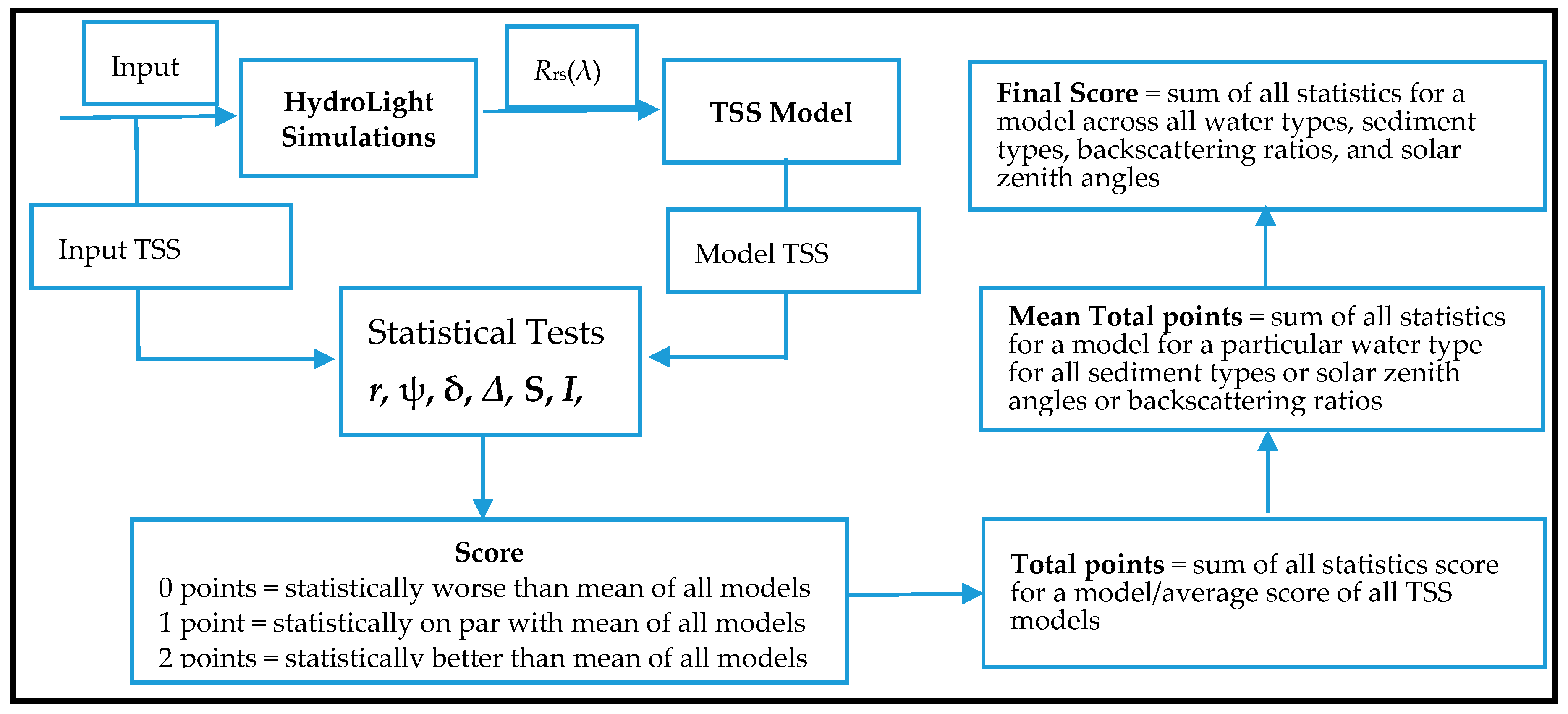
2.3. Statistical Tests and Scoring System

The statistical tests used to evaluate the performance of each TSS algorithm for different types of water described in Section 2.1.2 are based on the statistical tests used by Brewin et al. [44]. Further, to objectively rank the TSS algorithms we used the point scoring system of Brewin et al. [44]. The details of each statistical test and scoring system of each test adopted from [44] are described in the following sections. Further, to contain the effect of spurious TSS generated by some of the TSS models being applied outside their range, we only included TSS estimations that were between a lower bound available in each TSS model (zero for the TSS models which did not contain the lower bound) and an upper bound of twice the highest TSS concentration reportedly used to calibrate each TSS model.

2.3.1. Pearson Correlation Coefficient (r) Test

The point scoring system for the r test involves determining if the r-value for each TSS algorithm is statistically significant when compared with the mean r-value for all TSS algorithms. The statistical significance is determined through z-scores and the z-score is computed through Fisher’s r-to-z transformation using relationships between the r-values of two models and the total number of samples used to determine the r-values, described in [44] as:
z 1 = 0.5 log ( 1 + r 1 1 r 1 )
z 2 = 0.5 log ( 1 + r 2 1 r 2 )
z s c o r e = z 1 z 2 1 n 1 3 + 1 n 2 3
where r1 is the r-value of a specific TSS algorithm and r2 is the mean of all r-values from all the TSS algorithms. Similarly, n1 is the number of samples in a specific TSS algorithm and n2 is the mean number of samples from all TSS algorithms. In the event that the TSS model fails to produce a reasonable estimate of TSS within the accepted bounds of each TSS model when tested for a particular water type then in such cases the value of n1 can be different between two different water conditions, similarly, the value of n2 also changes as it is the average number of samples of all TSS models in that particular water type.
For algorithm comparison, a two-tailed test was performed using the z-score to determine the p-value. If the p-value was less than 0.05 then the r-values were considered as statistically significant and for each TSS algorithm that were statistically significant the following scores were assigned comparing the r-value and the mean r-value ( r ¯ ) of all TSS algorithms:
r test } 0 points i f r < r ¯ 1 point i f r = r ¯ 2 points i f r > r ¯

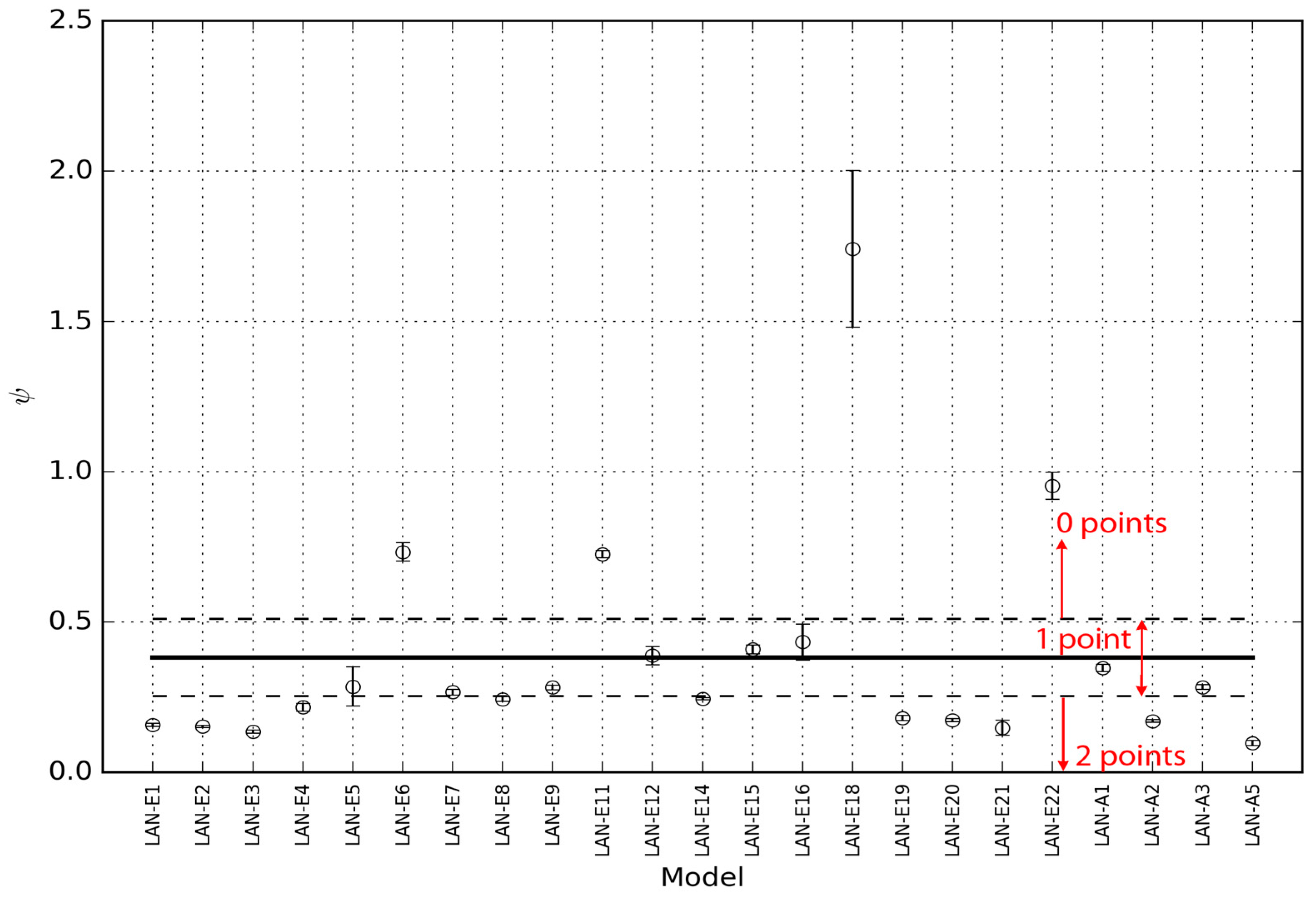
2.3.2. Root Mean Square Error (ψ) Test

The Root Mean Square Error (ψ) of a model estimate, yi, with respect to a true value, xi, can be computed using Equation (18):
ψ = 1 N i = 1 N ( y i x i ) 2
The 95% confidence intervals were also calculated for each TSS algorithm and the mean of all TSS algorithms. For each TSS algorithm, the following scoring points were assigned according to the conditions in Equation (19):
ψ t e s t   } 0   points   1   point   2   points   i f i f i f ψ ψ 95 % C I > ψ ¯ + ψ ¯ 95 % C I ψ ¯ ψ ¯ 95 % C I ψ ψ 95 % C I ψ ¯ + ψ ¯ 95 % C I   or ψ ¯ ψ ¯ 95 % C I ψ + ψ 95 % C I ψ ¯ + ψ ¯ 95 % C I ψ + ψ 95 % C I < ψ ¯ ψ ¯ 95 % C I
where ψ 95 % CI and ψ ¯ 95 % CI is the 95% confidence interval of ψ and mean—ψ ( ψ ¯ ) of all TSS algorithms respectively.
Figure 2 shows an example of scoring point classification for Landsat algorithms used in retrieving TSS concentration for the ψ—test.

2.3.3. The Bias (δ) Test

The bias (δ) of model estimate yi and true xi is calculated using Equation (20):
δ = 1 N i = 1 N ( y i x i )
For each TSS algorithm, following score points were awarded according to the conditions in Equation (21):
δ t e s t } 0   points 1   point   2   points   i f i f i f   δ 95 % CI > δ ¯ 95 % CI   AND   δ δ 95 % CI > 0 + δ 95 % CI   or   δ + δ 95 % CI > 0 δ 95 % CI δ 95 % CI < δ ¯ 95 % CI   or   0 δ ¯ 95 % CI δ + δ 95 % CI 0 + δ ¯ 95 % CI   or   0 δ ¯ 95 % CI δ δ 95 % CI 0 + δ ¯ 95 % CI δ 95 % CI < δ ¯ 95 % CI   AND   0 δ ¯ 95 % CI δ δ 95 % CI 0 + δ ¯ 95 % CI   or   0 δ ¯ 95 % CI δ + δ 95 % CI 0 + δ ¯ 95 % CI
where δ 95 % CI and δ ¯ 95 % CI is the 95% confidence interval of mean—δ ( δ ¯ ) of all TSS algorithms respectively. Further, to score one point only one conditions must be satisfied while to score two points both the conditions must be satisfied.

2.3.4. The Center-Pattern Root Mean Square Error (Δ) Test

The center-pattern Root Mean Square Error (Δ) is calculated using Equation (21):
Δ = 1 N i = 1 N { ( y i y ¯ ) ( x i x ¯ ) } 2
The 95% confidence intervals were also calculated for each TSS algorithm and the mean of all TSS algorithms. For each TSS algorithm, the following scores were assigned according to the conditions in Equation (23):
Δ t e s t } 0   points 1   point   2   points i f i f i f Δ Δ 95 % CI > Δ ¯ +   Δ ¯ 95 % CI Δ ¯   Δ ¯ 95 % CI Δ Δ 95 % CI Δ ¯ +   Δ ¯ 95 % CI   or   Δ ¯   Δ ¯ 95 % CI Δ + Δ 95 % CI Δ ¯ +   Δ ¯ 95 % CI Δ + Δ 95 % CI < Δ ¯ Δ ¯ 95 % CI
where Δ 95 % CI and Δ ¯ 95 % CI is the 95% confidence interval of Δ and mean—Δ ( Δ ¯ ) of all TSS algorithm respectively.

2.3.5. The Slope (S) and Intercept (I) of a Type-2 regression Test

The Slope (S) and Intercept (I) of a type-2 regression [64] were calculated using Equation (24):
Y = X × S + I
where Y is the TSS estimates derived from the TSS algorithms and X the true TSS. The following scores were assigned by comparing the S—value of each TSS algorithm and mean—S ( s ¯ ) value of all TSS algorithms.
S test } 0   points 1   point   2   points i f i f i f σ s > σ s ¯ AND S σ s > 1 + 2 σ s ¯ or S + σ s < 1 2 σ s ¯ σ s < σ s ¯ or 1 2 σ s ¯ S σ s 1 + 2 σ s ¯   or 1 2 σ s ¯ S + σ s 1 + 2 σ s ¯ σ s < σ s ¯ AND 1 2 σ s ¯ S σ s 1 + 2 σ s ¯   or   1 2 σ s ¯ S + σ s 1 + 2 σ s ¯
where σ s ¯ is the standard deviation of s ¯ from all TSS algorithms.
For the I parameter, for each TSS algorithm, the following scores were assigned according to the conditions in Equation (26).
I test } 0   points 1   point   2   points i f i f i f σ I > σ I ¯ AND I σ I > 0 + 2 σ I ¯ or I + σ I < 0 2 σ I ¯ σ I < σ I ¯ or 0 2 σ I ¯ I σ I 0 + 2 σ I ¯ or 0 2 σ I ¯ I + σ I 0 + 2 σ I ¯ σ I < σ I ¯ AND 0 2 σ I ¯ I σ I 0 + 2 σ I ¯ or 0 2 σ I ¯ I + σ I 0 + 2 σ I ¯
where σ I ¯ is the standard deviation of mean—I ( I ¯ ) from all TSS algorithms. Further, in the S and I—test in Equations (25) and (26), to score one point only one of the two conditions must be satisfied while to score two points both the conditions must be satisfied.

2.3.6. Percentage of Possible Retrievals (η)

The percentage of possible retrievals (η) was calculated using Equation (27):
η = N E N M × 100 %
where NE is the total number of TSS retrieved using each TSS algorithm from the total number of TSS concentrations (NM) considered in the study. For the point scoring system the following basis was followed:
η t e s t } 0   points 1   point   2   points i f i f i f η < η ¯ σ η ¯ η ¯ σ η ¯ η η ¯ + σ η ¯ η > η ¯ + σ η ¯
where η ¯ and σ η ¯ is the mean η-value and its standard deviation for all TSS algorithm in η-test.

2.3.7. Total Points

For objective comparison the performance of each TSS algorithm with respect to different water types, all points from each statistical test were added and normalized by the mean score of all TSS algorithms. Thus, a score of zero indicates that the TSS algorithm is performing lower than the mean of all TSS algorithms, a score of one indicates that the TSS algorithm is at par with the average of all TSS algorithms, and a score of 2 means the TSS algorithm is better than the mean of all TSS algorithms.
Further, to test the stability of the scoring systems used in this study, we used a bootstrap method [65], with 1000 runs and each time generating a new dataset by resampling via the replacement method for model generated TSS and HydroLight TSS. Each new dataset was tested using the statistical tests and scored using the scoring system described in Section 2.3. The results reported in the Section 3 are the mean values of the total points from the bootstrapping method with 2.5 and 97.5 percentiles reported as uncertainty estimates for 95% confidence limits.

2.3.8. Mean of Total Points
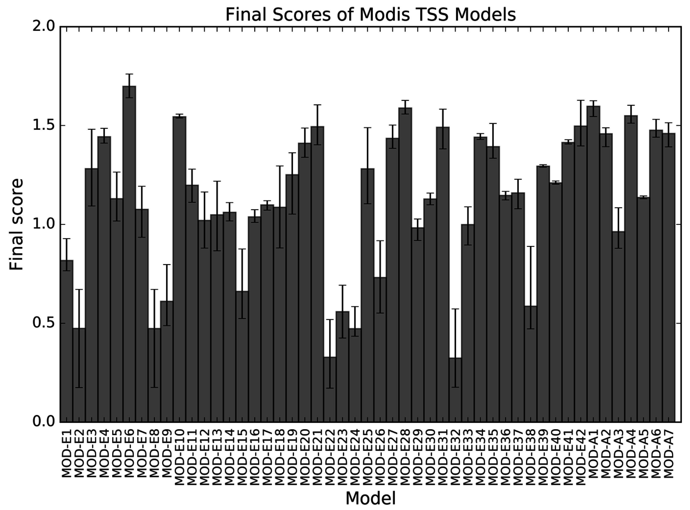
The mean of total points is achieved by averaging the score of each TSS model across different sediment types or solar zenith angles or backscattering ratios for the particular water classes described in Section 2.3.7. For example, in the case of different sediment types in CLASS-I water, the mean of total points in CLASS-I is an aggregate of total scores of each TSS model for different sediment types. For the case of different backscattering ratios and solar zenith angle, the mean of total points is an aggregate of each TSS model for different backscattering ratios and solar zenith angles, respectively, for a specific sediment type in a particular water class. The error bars in the mean of total points are the mean of uncertainty estimates of the total points obtained from the 95% confidence limit from the bootstrapping method.

2.3.9. Final Score

The final score is the aggregate of the mean of total points across all water classes for different sediment types, backscattering ratios and solar zenith angles. For example, the final score for MOD-E1 is derived as the mean from the aggregate score of MOD-E1 at five different sediment types, backscattering ratios, and solar zenith angles across all five different water classes. The error bars are the standard deviation of errors from the mean of total points across all five different water classes. Figure 3 shows an illustration of the point score system adapted from [44] and used in comparing TSS models in this study. The error bars in the Final score are the mean of uncertainty estimates from the mean of total points.

3. Results

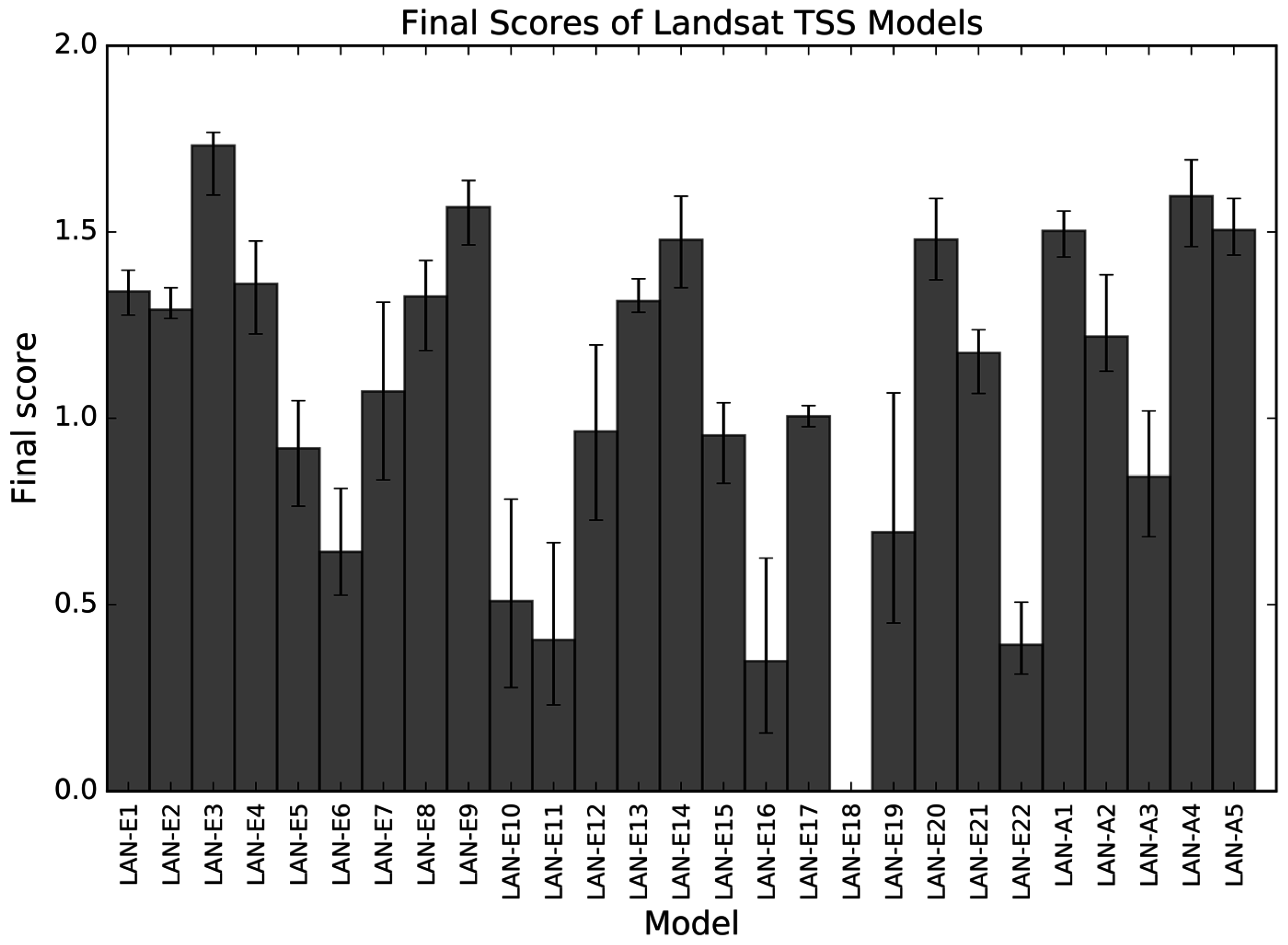
3.1. TSS Model Comparisons

Figure 4 and Figure 5 show the quantitative comparison between the models using the final scores which are aggregates of the total scores from different sediment types, backscattering ratios, and solar zenith angles across all five different water classes for MODIS and Landsat-based models respectively. The final results presented in Figure 4 and Figure 5 are indications of the overall performance of the TSS models when weighted across different water types, sediment types and backscattering ratios. The detailed results of individual model performance in respective sediment types, backscattering ratios, and water types are presented in Supplementary Material, S11. In addition, the Supplementary Materials S1–S10 also provide the detailed statistical test results for each TSS model.
From the final scores displayed in Figure 4 and Figure 5 we can visually observe that there are clearly high and low performing models. The high performing MODIS TSS models with final scores greater than 1.5, in the order of highest to lowest final score, are MOD-E6, MOD-A1, MOD-E28, MOD-A4, MOD-E10, and MOD-E42 and low performing MODIS TSS models with scores less than 0.5 are MOD-E8, MOD-E2, MOD-E24, MOD-E22 and MOD-E32. For the Landsat TSS models, LAN-E3, LAN-A4, LAN-E9, LAN-A5, and LAN-A1 have final scores greater than 1.5 while LAN-E11, LAN-E22, LAN-E16, and LAN-E18 have final scores less than 0.5. In the final scores of low performing TSS models, the LAN-E18 model has scores of zeros which shows that LAN-E18 failed to derive TSS within the acceptable TSS bounds of 0.4–5.8 mg/L. We suspect the published algorithm includes an error. The overall ranking of the TSS models using the final scores for each TSS model is also presented in Table B1 and Table B2 for MODIS and Landsat respectively. Further, Table B1 and Table B2 provides mean total scores for different sediment types, backscattering ratios, and solar zenith angles in all five water classes for respective TSS model.
With respect to the results displayed in Figure 4 and Figure 5, without the inclusion of error bars the distinction between the high performing TSS models is clear and we can easily compare the scores of each TSS model to obtain a ranking. For instance, in Figure 4 and Figure 5, the MOD-E6 and LAN-E3 are the highest scoring models with final scores of 1.70 and 1.73 respectively. However, on inclusion of the error bars, all high performing TSS models may be considered comparable and difficult to separate in terms of robustness, thus may all be ranked equally. Likewise, the case is similar for low performing TSS models where their error bars overlap. Further, we observe that two and three of the top five high scoring TSS models in MODIS and Landsat respectively are semi-analytic while none of the semi-analytic models were in the bottom five low scoring models.

3.2. Evaluation of Models

3.2.1. Model Evaluation Using HydroLight Data

The five high and low scoring models from MODIS and Landsat TSS models were selected to further evaluate their performance. From all available HydroLight data discussed in Section 2.1.2, the aforementioned high scoring TSS models were evaluated for their Relative Error (RE) between model-derived and HydroLight TSS. From the results presented in Table 3 we observe that there is high variability in the RE results amongst the respective MODIS and Landsat TSS models. The differences in the Smallest Relative Error (SRE) for high scoring TSS models were not as large as the differences within the MARE and Largest Relative Error (LRE). The MARE ranged from a low of 69.96% to a high of 481.82% while the SRE and LRE ranged from 15% to 63.14% and 139.35% to 1109.80% respectively. In the low scoring models, the high variability in the RE was observed with the MARE for low performing models ranging from 106.43% to 1832.79% while the SRE and LRE ranged from 39.90% to 213.54% and 118.16% to 6778.93% respectively. In both MODIS and Landsat high scoring models, the LRE results were for backscattering ratios of 0.001 and for Bukata type sediment. The SRE results were for backscattering ratios of 0.01 and calcareous sand sediment. Further, for the SRE in both the high and low performing TSS models, we observe that the high and low performing TSS models scored reasonably well in either one of the categories in sediment types, backscattering ratios, solar zenith angle and water classes. For instance, the low performing LAN-E22 scored higher than most of the high scoring TSS models in SRE results which indicated that LAN-E22 retrieves better in one of the water types.
The TSS derived using real satellite-data are bound by uncertainty related to observational, instrumental, measurement and data processing errors, the latter largely associated with the atmospheric correction procedure [66]. Thus, to assess the tolerance of high and low performing TSS models to the uncertainties in Rrs, which is the key input in derivation of the TSS concentration, we simulated the effect of Rrs uncertainty (󠄢ΔRrs) by varying the Rrs by ±10%, ±20% and ±50% of the HydroLight generated Rrs at each of the MODIS and Landsat bands. The Rrs ± ΔRrs was used in deriving TSS concentration and compared with HydroLight input TSS to calculate the Absolute Relative Error (ARE) of the TSS model. Table 3 reports the ARE and the MARE of HydroLight Data Validation as defined in Equation C2 in Appendix C. In general, we observe that with the increase in ΔRrs the ARE also increases and the errors are higher for +ΔRrs than −ΔRrs. The ARE for high scoring TSS models ranged from 33.14% to 1974.47% while for low scoring TSS models it ranged from 82.69% to 12747.84% which shows both high and low performing TSS models are not impervious to uncertainty in Rrs measurements. However, high scoring TSS models show better tolerance to ΔRrs than the low scoring TSS models. The details of the TSS models deviation in estimating TSS concentration from the error-free HydroLight data with ΔRrs are shown in Table 3.

3.3.2. Model Evaluation Using In situ Data

As part of a regional water monitoring program, in situ reflectance and TSS measurements were carried out for the waters off the coast of northern Western Australia to develop regional TSS models (see MOD-A1 and LAN-A1 in Appendix A) [67]. The details of the in situ measurements and regional TSS model developed using in situ data can be obtained from [67]. A set of high scoring models (MOD-E10, MOD-A4, LAN-E9, and LAN-A5) and low scoring models (MOD-E1, MOD-E38, LAN-E6, and LAN-A3) were selected to compare with MOD-A1 and LAN-A1 in the context of in situ data comparisons. These subsets of models were selected because the reflectance bands used by other high scoring models were beyond the available reflectance bands in the in situ data. Table 4 shows the Mean RE results obtained from each of the model evaluations against in situ data. Table 4 displays a high variability in the Mean RE for model comparisons for high scoring models with in situ data, from a low of 43.11% for LAN-E9 to a high of 102.59% for LAN-A5. When compared with the regional model’s MOD-A1 and LAN-A1 MARE results, we see that both the high scoring TSS models MOD-E10 and LAN-E9 and low scoring TSS models LAN-E6 and LAN-A3 were comparable. However, the results presented in Table 4 also show the extreme variability observed in the Mean RE for the low scoring models with a low of 35.62% and a high of 256%.

4. Discussion

4.1. Data and Methodological Limitation

The data used in this study to quantitatively compare TSS models have been generated using the widely used [68,69] in-water radiative transfer model HydroLight 4.2. The simulated data do not encompass all different water types in which each TSS model was developed to be used, however, it does provide us with a dataset that is independent of the data that has been used to parameterize the models to avoid biases in the results. To include all the models in comparisons, the simulated data were extrapolated to the NIR region of the spectrum using the methods discussed in Section 2.1.2. The extrapolation of reflectance data can introduce unrealistic values if the underlying assumptions of the spline extrapolation methodology does not hold true for the NIR regions. The extrapolation of the data is not ideal when used in modelling remote sensing products but the error for extrapolation had a MARE of 4.0% which was considered to be acceptable for this study. The ideal case for data for model comparisons would be to use a real global water data base, which is currently not available. The NOMAD dataset (http://seabass.gsfc.nasa.gov/) that is currently the most extensive dataset of in situ reflectance measurement and in-water variables did not contain the TSS measurements essential for this study.
The use of the objective methodology [44] of comparing models, used in this study to compare TSS models, can aid users in selection of TSS models that are best suited for waters of regional interest in the absence of means and a method to produce their own regionally tuned TSS algorithms. However, the objective methodology used here is not without limitations, as discussed by [44] with respect to using average performance to classify between high and low performing models. The very low performance of one particular model would affect the average of all other models to the extent that it becomes difficult to differentiate scores between models. For example, in Figure S11.1 for the score of MODIS TSS models in yellow clay, MOD-E1-2, E8-9, E15, E22-24, E32, and E38 all have low scores which increases the score of other TSS models making it difficult to differentiate among high scoring models. This problem is further exacerbated when the majority of TSS models score low which makes the few remaining high scoring models to appear similar in score, which is the case in Figure S11.22 for bb/b of 0.001.
The objective classification was conducted on a case by case basis for different water types, sediment types, solar zenith angles, and backscattering ratios. The overall low performance of models in the final scores in Figure 4 and Figure 5 does not necessarily mean that low performing TSS models scored less in all the categories used in deriving the final score. For example, in Figure 5, LAN-E22 scored a very low final score when compared to other TSS models, but when considering specific results as presented in Figures S11.16–S11.20, LAN-E22 received a score at least comparable with most of the best performing models in all water classes for the red clay sediment type. Likewise, similar cases can be ascertained for all the respective TSS model’s scores for specific water classes, sediment types, backscattering ratios and solar zenith angle (Results provided as Supplementary Material S11 for other overall low scoring TSS models in Figure 4 and Figure 5). An additional disadvantage of the objective methodology used here is that the final score does not necessarily show the performance of all models in different categories considered, it shows only the relative performance of models in comparison with the mean scores of TSS models. In Figure S11.1, we observe that almost all TSS models score relatively higher total points for brown earth and lower for Bukata sediment types when compared with other sediments.
To account for the methodological uncertainties from the range of univariate statistical tests described in Section 2.3, we used a bootstrapping method [44,65] which generates the confidence limit in the final score. The results from the 1000 bootstrap runs presented in all the score charts shows that the mean score of models did not vary significantly for each different run, the ranges of 95% confidence limits were smaller for most of the models. Further, to limit the effect of spurious TSS values derived by some of the models, especially models with exponential and power functions, we filtered out any derived TSS value below a minimum of 0.001 mg/L and greater than a twice the maximum TSS concentration of each TSS model. Filtering out the spurious results can artificially inflate the final scores because only values that are within the upper and lower bounds would be considered for statistical tests. However, the possible percentage retrieval test discussed in Section 2.3.6 negate such an effect because filtering out spurious results would result in lower possible percentage retrieval and lower score in the percentage retrieval test.

4.2. TSS Model Selection Guidelines

Even though there were clearly distinct higher and lower performing TSS models from the final score chart presented in Figure 4 and Figure 5, the performance of individual models varied widely when viewed against respective water types, sediment types, and backscattering ratios. The results presented in Figure 4 and Figure 5 can be of use to the end-users who are clearly interested in TSS models that are robust enough to be used in waters for which they have little or no information of their optical and physical properties to generate TSS products. Figure 4 and Figure 5 indicate that the MODIS TSS models MOD-E6, MOD-A1, MOD-E28, MOD-A4 and MOD-E10 and the Landsat TSS models LAN-E3, LAN-A4, LAN-E9, LAN-A5 and LAN-A1 are ranked the highest in terms of likely suitability for estimating TSS concentration of unknown water types. An example of the selection of high performing TSS models using a real water dataset was demonstrated in Section 3.3.2 and it can be seen that the results varied widely among the high scoring TSS models, with MOD-E10 and LAN-E9 producing results within a MARE of 46.20% and 43.11% and other higher scoring models producing results as high as 102.59%. Considering the retrieval error of TSS concentrations from MODIS algorithms are typically reported as in the range of ~18.0% to ~61% for many studies conducted in the last decade [35,37,38,46,47], we consider the regional TSS models MOD-A1 and LAN-A1, and the empirical models MOD-E10 and LAN-E9 as being the most appropriate for the waters in the north of Western Australia.
However, readers with prior information of water and sediment types can use information provided in S11, and Table B1 and Table B2 as a guideline in selecting the model that is best suited for that particular water type. The difference in Relative Error between the high and low scoring models validated using HydroLight data and the in situ data showed that there is a huge difference between the two. The best performing model from the high scoring models shows that TSS can be estimated with a Mean RE between 69.96% and 481.82% (for different water conditions), but the low scoring model’s results can vary dramatically within a Mean RE ranging from 106.43% to 1832.79%. The high Mean RE for low scoring models does not necessarily mean that the low scoring model performs low for all waters types. The low scoring TSS model’s performance in one category or more can be significantly better than other models, but overall on average the model performs poorly when compared with high scoring models across all water types. For example, the low scoring model LAN-E22 displays the Smallest RE of 19.41% which is certainly better than the Smallest RE of most of the high scoring model’s Smallest RE. Thus, with prior knowledge of water types and bio-geochemical properties of the region, we can select a TSS model from both high and low performing TSS models presented in Table B1 and Table B2 that have higher scores in the water that are similar to the region where TSS model would be applied.
The results also showed that semi-analytic models were generally higher in ranking when compared with empirical models. The reason for most semi-analytic models performing better than empirical models can be attributed to the fact that semi-analytic models, by design, were based on radiative transfer theory [38,70] and one or more parameters were calibrated using general in situ bio-optical properties representative of a wide range of global waters [7,38].

5. Conclusions

In summary, in this study we have applied an objective methodology to compare the TSS models and their suitability in use for retrieving TSS in the absence of a regionally tuned TSS model. From the study we have identified the MODIS TSS models MOD-E6, MOD-A1, MOD-E28, MOD-A4 and MOD-E10 and the Landsat TSS models LAN-E3, LAN-A4, LAN-E9, LAN-A5 and LAN-A1 as suitable for estimating TSS concentration in waters with no prior knowledge of bio-optical or bio-geochemical properties. The results from this study highlighted the impact of “local tuning” of algorithms, showing that some low scoring models performed better than the high scoring models in one or more specific sediment, backscattering, solar zenith and water types. The results from this study can be used to ascertain which TSS models perform well in particular water types, sediment types and backscattering ratios for use in aiding the selection of a TSS model suited for use in a particular water type. In addition, the results also show that the semi-analytic TSS models are generally better than empirical TSS models in deriving TSS estimation in unknown water types.

Supplementary Materials

The following supplementary materials are available online at www.mdpi.com/2072-4292/8/10/810/s1. Figure S1.1: Scatter plot of MODIS-TSS models in CLASS-I water for brown earth sediment with bb/b ratio of 0.018 and solar zenith angle of 30°, Figure S1.2: Scatter plot of MODIS-TSS models in CLASS-I water for bukata sediment with bb/b ratio of 0.018 and solar zenith angle of 30°, Figure S1.3: Scatter plot of MODIS-TSS models in CLASS-I water for calcareous sand sediment with bb/b ratio of 0.018 and solar zenith angle of 30°, Figure S1.4: Scatter plot of MODIS-TSS models in CLASS-I water for red clay sediment with bb/b ratio of 0.018 and solar zenith angle of 30°, Figure S1.5: Scatter plot of MODIS-TSS models in CLASS-I water for yellow clay sediment with bb/b ratio of 0.018 and solar zenith angle of 30°, Figure S1.6: Scatter plot of MODIS-TSS models in CLASS-I water for calcareous sand sediment with bb/b ratio of 0.001 and solar zenith angle of 30°, Figure S1.7: Scatter plot of MODIS-TSS models in CLASS-I water for calcareous sand sediment with bb/b ratio of 0.01 and solar zenith angle of 30°, Figure S1.8: Scatter plot of MODIS-TSS models in CLASS-I water for calcareous sand sediment with bb/b ratio of 0.05 and solar zenith angle of 30°, Figure S1.9: Scatter plot of MODIS-TSS models in CLASS-I water for calcareous sand sediment with bb/b ratio of 0.1 and solar zenith angle of 30°, Figure S1.10: Scatter plot of MODIS-TSS models in CLASS-I water for calcareous sand sediment with bb/b ratio of 0.081 and solar zenith angle of 15°, Figure S1.11: Scatter plot of MODIS-TSS models in CLASS-I water for calcareous sand sediment with bb/b ratio of 0.081 and solar zenith angle of 45°, Figure S1.12: Scatter plot of MODIS-TSS models in CLASS-I water for calcareous sand sediment with bb/b ratio of 0.081 and solar zenith angle of 60°; Figures in S2, S3, S4 and S5 all aforementioned Figures in S1 in CLASS-II, CLASS-III, CLASS-IV and CLASS V water type. In S6 and S10 are similar aforementioned Figures in S1–S5 but for Landsat TSS models; Figure S11.1–S11.5: Total scores for different sediment and the average score across all five sediments in CLASS-I, CLASS-II, CLASS III, CLASS IV and CLASS V water type respectively, Figures S11.6–S11.10: Total scores for different backscattering ratios and the average scores across all backscattering ratios in CLASS-I, CLASS-II, CLASS III, CLASS-IV and CLASS-V water type respectively, Figures S11.11–S11.15: Total scores for different solar zenith angles and the average scores across all solar zenith angles in CLASS-I, CLASS-II, CLASS-III, CLASS IV, and CLASS-V water type respectively, Figures S11.16–S11.30 are similar to Figures S11.1–S11.15 but for Landsat TSS models.

Acknowledgments

This study was funded by the Western Australian Marine Science Institute through Dredging Science Node Project 2/3. The authors wish to acknowledge Curtin University for providing a postgraduate research scholarship to Passang Dorji.

Author Contributions

The general conception of this study was designed by both the authors. Passang Dorji with guidance from Peter Fearns worked on HydroLight simulation, data processing and data analysis. The manuscript was written by Passang Dorji with critical feedback and revision from Peter Fearns.

Conflicts of Interest

The authors declare no conflict of interests.

Appendix A

Table A1. The summary of TSS algorithms mentioned in Section 2.2.
AlgorithmReferenceLocationTSS Range (mg/L)Bands/AlgorithmsRegression Coefficient (R2)ErrorN
MOD-E1Kumar, et al. (2016) [71]Chilika Lagoon, India 3.9–161.7 T S S = 13181 R r s ( B 1 ) 2 1408.6 R r s ( B 1 ) + 44.15 0.915RMSE = 2.64 mg/L54
MOD-E2Ayana, et al. (2015) [40]Gumera catchment, Lake Tana, Ethiopia ~5–255 T S S = 2371 ρ ( B 2 ) 62.8 0.95SE = 10.77 mg/L54
MOD-E3Chen, et al. (2015) [22]Estuary of Yangtze River and Xuwen Coral Reef, China5.8–577.2 l o g ( T S S ) = b + b 2 4 a ( c y ) 2 a } R r s ( B 1 ) < 0.025 log ( T S S ) = b + b 2 4 a ( c y ) 2 a } R rs ( B 1 ) > 0.025 a = 0.334 , b = 1.0046 , c = 0.8251 , ( b 2 4 a ( c y ) ) 0 y = log ( R r s ( B 2 ) ) / log ( R r s ( B 1 ) ) 0.752RMSE = 2.1 mg/L
RMSE = 38.6 mg/l
40
MOD-E4Zhang, et al. (2016) [72] and Shi, et al. (2015) [21]Lake Taihu, China 1.7–343.9 T S S = 9.65 exp ( 58.81 R r s ( B 1 ) ) 0.70RMSE = 14.0 mg/L150
MOD-E5Choi, et al. (2014) [34]Mokpo coastal area, Korea1.03–193.10 T S S = 1.545 exp ( 179.53 R r s ( B 1 ) ) 0.92-96
MOD-E6Feng, et al. (2014) [35]Yangtze estuary4.3–1762.1 T S S l o w = 2.49 exp ( 97.19 R r s ( B 1 ) ) } T S S < 10 ( m g / l ) T S S h i g h = 57.58 exp ( 3.48 ( R r s ( B 2 ) / R r s ( B 1 ) ) ) } T S S > 150 ( m g / l ) T S S m i d = α × T S S l o w + β × T S S h i g h } 50 < T S S < 150 ( m g / l ) α = ln ( T S S l o w / 50 ) ln ( 150 / 50 ) , β = ln ( 150 / T S S l o w ) ln ( 150 / 50 ) 0.88 (low)
0.93 (high)
RMSE = 27.7%78
MOD-E7Hudson, et al. (2014) [23]Fjord in Southwest Greenland1.2–716 T S S = 1.80 exp ( 19.11 ( R r s ( B 1 ) + R r s ( B 2 ) ) 0.84-143
MOD-E8Kaba, et al. (2014) [31]Lake Tana, Ethiopia ~5–255 T S S = 2371 × ρ ( B 2 ) 62.8 0.95RMSE = 16.5 mg/L54
MOD-E9Lu, et al. (2014) [73]Bohai Sea, China~<160 T S S = exp ( R r s ( B 1 ) 0.0123 0.0038 ) 0.75RE ≤ 20%627
MOD-E10Park and Latrubesse, (2014) [32]Amazon River system 30–150 T S S = 27.05 exp ( 7.83 ρ ( B 1 ) ) 0.88RMSE = 6.2 mg/L232
MOD-E11Sokoletsky, et al. (2014) [74]Yangtze river estuary0–2500 T S S = 1 0 ( 2 × [ R r s ( B 1 ) / R r s ( B 4 ) ] ) - 361
MOD-E12Chen, et al. (2014) [61]Bohai Sea4–106.4 T S S = 3 × 10 8 x 3 2 × 10 6 x 2 + 5453.3 x + 3.8825 x = ρ w ( B 15 ) 1.107 ρ w ( B 16 ) 0.954RMS = 30.12%48
MOD-E13Cui, et al. (2013) [75]Ponyang lake, China0–141.9 T S S = 1.063 exp ( 27.859 ρ ( B 1 ) ) 0.91SE = 11.20 mg/L54
MOD-E14Kazemzadeh, et al. (2013) [76]Bahmanshir River, Iran30–500 T S S = 22.92 ρ ( B 1 ) 0.82 0.63RMSE = 261.8423
MOD-E15Raag, et al. (2013) [17]Pakri Bay, Gulf of Finland0–10 T S S = 592.54 ρ ( B 1 ) ) + 1.1136 0.52 77
MOD-E16Qui (2013) [46]Yellow River Estuary, China1.9–1896.5 T S S = exp ( 1.1932 ( R r s ( B 12 ) R r s ( B 14 ) ) 0.875 ) 0.95MAE = 24.5 mg/L81
MOD-E17Villar, et al. (2013) [77]Maderia River25–622 T S S = 1020 ( R r s ( B 2 ) R r s ( B 1 ) ) 2.94 0.62-282
MOD-E18Min, et al. (2012) [78]Saemangeum coastal area, Korea0.1–55 T S S = 0.24 exp ( 188.3 R r s ( B 12 ) ) 0.90-88
MOD-E19Ondrusek, et al. (2012) [62]Chesapeake Bay4.5–14.92 T S S = 3.8813 ( n L w ( 645 ) ) 3 13.822 ( n L w ( 645 ) ) 2 + 19.61 ( n L w ( 645 ) ) 0.95MPD = 4.2%35
MOD-E20Son and Wang, (2012) [39]Chesapeake Bay1.0–20 T S S = 1.7 + 5.263 K d ( 490 ) 0.77STD = 0.4815,720
MOD-E21Wang, et al. (2012) [60]Hangzhou Bay, China133–1,950 T S S = 1.4599 ( R r s ( B 1 ) R r s ( B 2 ) ) 2.3874 0.82 35
MOD-E22Chen, et al. (2011) [24]Apalachicola Bay, USA1.29–208 log ( ρ ( B 2 ) / log ( ρ ( B 1 ) ) = 0.1325 log ( T S S ) 2 + 0.7429 log ( T S S ) + 0.6768 0.86RMSE = 4.76 mg/L32
MOD-E23Chen, et al. (2011) [36]Apalachicola Bay, USA1.29–208 log ( ρ ( B 2 ) / log ( ρ ( B 1 ) ) = 0.4339 log ( T S S ) + 0.8288 0.8RMSE = 4.7925
MOD-E24Jiang and Liu(2011) as cited in [22]Poyang Lake, China0–40 T S S = 1365.5 x 2 369.08 x + 27.216 x = R r s ( B 3 ) + R r s ( B 4 ) 0.81-27
MOD-E25Siswanto, et al. (2011) [79]Yellow and East China Sea0.04–340.07 T S S = 10 ( 0.649 + 25.623 ( R r s ( B 12 ) + R r s ( B 13 ) ) 0.646 ( R r s ( B 10 ) R r s ( B 12 ) ) ) 0.92RPD = 15.7%223
MOD-E26Zhao, et al. (2011) [80]Mobile Bay estuary, Alabama0–87.8 T S S = 2.12 exp ( 42.92 ρ ( B 1 ) ) 0.781RMSE = 5.4263
MOD-E27Petus, et al. (2010) [81] and Petus, et al. (2014) [37]Bay of Biscay, France0.3–145.6 T S S = 12450 R r s ( B 1 ) 2 + 666.1 R r s ( B 1 ) + 0.45 0.97RMSE = 61%74
MOD-E28Wang and Lu (2010) [25]Yangtze River, China45–909 T S S = 61.369 exp ( 0.2623 x ) x ( % ) = ρ ( B 2 ) ρ ( B 5 ) 0.78RRMSE = 36.5%35
MOD-E29Wang, et al. (2010) [82]Apalachicola Bay, USA1–64 log ( T S S ) = 1.5144 ( log ( ρ ( B 2 ) ) / log ( ρ ( B 1 ) ) ) 0.5755 0.72-16
MOD-E30Wang, et al. (2010) [47]Middle and Lower Yangtze River, China75–881 T S S = 60.24 x 23.03 x ( % ) = ρ ( B 2 ) ρ ( B 5 ) 0.73RMSE = 29.7%153
MOD-E31Zhang, et al. (2010) [83]Yellow and East China Sea0.68–27.2 log ( T S S ) = s 0 + s 1 ( R r s ( B 4 ) + R r s ( B 1 ) ) + s 2 ( R r s ( B 10 ) / R r s ( B 4 ) ) s 0 = 0.6311 , s 1 = 22.2158 , s 2 = 0.5239 0.87ARE = 26%81
MOD-E32Chen, et al. (2009) [63]Apalachicola Bay, USA1.29–208 log ( ρ ( B 2 ) / log ( ρ ( B 1 ) ) = 0.1356 log ( T S S ) 2 + 0.7402 log ( T S S ) + 0.6836 0.853RMSE = 5.5 mg/L25
MOD-E33Chu, et al. (2009) [84]Kangerlussuaq Fjord, Greenland~500 T S S = 10 ( R r s ( B 1 ) 1.6 7.5 ) ---
MOD-E34Doxaran, et al. (2009L) [85]Gironde Estuary, France77–2182 T S S = 12.996 exp ( R r s ( B 2 ) / ( 0.189 R r s ( B 1 ) ) ) 0.89RMSE: 18%–22%204
MOD-E35Jiang, et al. (2009) [86]Taihu Lake, China0–170 T S S = 10 ( 0.3568 ln ( R r s ( B 2 ) + 3.3431 ) 0.81ARE = 20.5%56
MOD-E36Liu and Rossiter (2008) as cited in [22]Poyang Lake, China15.6–518.8 T S S = 7167 ρ ( B 1 ) 42.0 0.91-25
MOD-E37Wang, et al. (2008) [87]Hangzhou Bay, China17–6949 T S S = exp ( 43.233 R r s ( B 2 ) + 1.396 ) 0.76RMSE = 424 mg/L25
MOD-E38Wu and Cui (2008) as cited in [22]Poyang Lake, China0-142 T S S = 86236.23 ( R r s ( B 1 ) ) 3 15858.70 ( R r s ( B 1 ) ) 2 + 1005.29 ( R r s ( B 1 ) ) 15.67 0.92-42
MOD-E39Kutser, et al. (2007) [26]Muuga and Sillmae Port, Estonia2–8 T S S = 349.83 ρ ( B 1 ) + 2.9663 0.86-11
MOD-E40Liu, et al. (2006) [58]Middle Yangtze River, China23.4–61.2 T S S = exp ( 2.495 x + 1.81 ) x = ρ ( B 1 ) ρ ( B 2 ) ρ ( B 1 ) + ρ ( B 2 ) 0.72RE = 34.7%41
MOD-E41Sipelgas, et al. (2006) [27]Parki Bay, Finland3–10 T S S = 110.3 ρ ( B 1 ) + 2.0 0.58-48
MOD-E42Miller and Mckee, (2004) [3]Northern Gulf of Maxico, USA1.0–55.0 T S S = 1140.25 × R r s ( B 1 ) 1.91 0.89RMSE = 4.74 mg/L52
MOD-A1Dorji, et al. (2016) [67]Onslow, Western Australia2.4–69.6 T S S = 23.47 ( x ( B 1 ) 1 x ( B 1 ) ) 1 0.69 ( x ( B 1 ) 1 x ( B 1 ) ) | x ( B 1 ) = g 1 + ( g 1 ) 2 + 4 g 2 r r s ( B 1 ) 2 g 2 g 1 = 0.084 , g 2 = 0.17 , a n d r r s ( B 1 ) = R r s ( B 1 ) / ( 0.52 + 1.7 R r s ( B 1 ) ) 0.85MARE = 33.33%48
MOD-A2Han, et al. (2016) [88]Europe, French Guiana, Vietnam, North Canada, and China0.154–2627 T S S = W L T S S L + W H T S S H W L + W H W L = { 1 , i f R r s ( B 1 ) 0.03 s r 1 0 , i f R r s ( B 1 ) 0.04 s r 1 log 10 ( 0.04 ) log 10 ( R r s ( B 1 ) ) , o t h e r w i s e | T S S L = 404.4 ρ w ( B 1 ) 1 ρ w ( B 1 ) / 0.5 W H = { 0 i f R r s ( B 1 ) 0.03 s r 1 1 , i f R r s ( B 1 ) 0.04 s r 1 log 10 ( R r s ( B 1 ) ) log 10 ( 0.03 ) , o t h e r w i s e | T S S H = 1214.669 ρ w ( B 1 ) 1 ρ w ( B 1 ) / 0.3394 -MRAD = 51.9-59%TSSL = 366
TSSH = 46
MOD-A3Shen, et al. (2014) [89]Yangtze estuary, China- R r s = α β × T S S 1 + β × T S S + 1 + 2 β × T S S R r s ( B 2 ) } α = 0.1038 , β = 1.8042 0.91RMSE = 0.0048 (sr−1)144
MOD-A4Vanhellemont and Ruddick (2014) [11]Southern North Sea, UK0.5–100 T S S = 258.85 ρ ( B 1 ) 1 ρ ( B 1 ) / 0.1641 ρ ( B 1 ) = 0.529 × π × r r s ( B 1 ) ---
MOD-A5Chen, et al. (2013) [56]Changjiang River Estuary, China70–710 T S S = 1.7492 ( R r s ( B 16 ) 1 R r s ( B 15 ) 1 ) 1 + 0.0912 0.89MRE = 28.99%20
MOD-A6Katlane, et al. (2013) [90]Gulf of Gabes0.7–30 T S S = 62.86 ( ρ ( B 1 ) ( 0.1736 ρ ( B 1 ) ) ) ρ ( B 1 ) = π R r s ( B 1 ) --56
MOD-A7Nechad, et al. (2010) [38]Southern North Sea1.24–110.27 T S S = 400.75 ρ ( B 1 ) 1 ρ ( B 1 ) / 0.1774 + 1.02 ρ ( B 1 ) = 0.539 × π r r s ( B 1 ) 0.80RMSE = 11.23 mg/L
MRE = 38.9%
72
LAN-E1Cai, et al. (2015) [91]Hangzho Bay, China203–481 ln ( T S S ) = 0.01113115 × L ( T M 4 ) + 4.794229 0.951-35
LAN-E2Cai, et al. (2015) [92]Hangzho, Bay179–389.58 T S S = 314.435 ρ ( T M 3 ) + 3805.982 ρ ( T M 4 ) + 28.54 0.976-27
LAN-E3Kong, et al. (2015) [7]Gulf of Bohai Sea2.1–208.7 T S S = 5.184 + 1349.63 R r s ( T M 4 ) + 614561.673 [ R r s ( T M 4 ) ] 2 0.844RMSE = 5.5970
LAN-E4Kong, et al. (2015) [93]Caofeidian, Bohai Sea4.3–104.1 T S S = 296.29 x 2 272.62 x + 70.939 x = R r s ( T M 3 ) / R r s ( T M 2 ) 0.977RMSE = 7.22 mg/L
MRE = 25.35
LAN-E5Lim and Choi (2015) [94]Nakdong River, South Korea~3–14 T S S = 11.80 50.608 ρ ( O L I 2 ) + 14.58 ρ ( O L I 5 ) 4.764 ρ ( O L I 5 ) / ρ ( O L I 3 ) 0.74RMSE = 1.4048
LAN-E6Wu, et al. (2015) [9]Dongting Lake, China0–63.2 T S S = 1.1034 × exp ( 23.61 × ρ ( O L I 4 ) ) 0.91RMSE = 4.41 mg/L52
LAN-E7Zheng, et al. (2015) [95]Dongting Lake, China4.0–101 T S S = 4616.4 × R r s ( T M 4 ) 4.362 0.82MAPE = 21.3%
RMSE = 7.01 mg/L
42
LAN-E8In-Young, et al. (2014) [96]Old Women Creek Estuary, Ohio, US1.0–278 T u r b = 14.44 × ρ ( % , E T M 4 ) + 7.61 T u r b = 1.03 T S S 3.54 0.65 11
LAN-E9Zhang, et al. (2014) [10]Yellow river estuary1.0–1500 log 10 ( T S S ) = 44.072 × R r s ( T M 3 + 0.1591 ) 0.9672MRE = 26.1%44
LAN-E10Hao, et al. (2013) [97] Yangtze Estuary, China~40.0–750 R ( B 4 ) = 0.0444 + 32.7736 × [ T S S / ( 51.6753 + T S S ) ] 32.7260 × [ T S S / ( 51.6753 + T S S ) ] × exp ( 0.0000012081 × T S S ) 0.8175ARE = 36.8317
LAN-E11Hicks, et al. (2013) [98]Waikato River, New Zealand 2.0–962 T S S = 52.817 + 1449.4 ρ ( E T M 4 ) 0.939RMSE = 21.335
LAN-E12Min, et al. (2013) [78]Saemangeum coastal area, Korea0.1–55 T S S = 0.24 exp ( 188.3 R r s ( T M 2 ) ) 0.90-88
LAN-E13Miller, et al. (2011) [99]Albemarle-Pamlico Estuarine System, North Carolina, USA~5.0–30 T S S = 1.7 + 684.76 ρ ( % , E T M 3 ) 0.87-599
LAN-E14Li, et al. (2010) [100]Changjiang Estuary~1.5–560 1 o g 10 ( T S S ) = 0.892 + 6.2244 x x = [ ρ ( E T M 2 ) + ρ ( E T M 3 ) ] [ ρ ( E T M 2 ) / ρ ( E T M 3 ) ] 0.915-21
LAN-E15Wang, et al. (2009) [12]Yangtze river, China22–2610 ln ( T S S ) = 3.18236 × ln ( % , ρ w ( E T M 4 ) ) 0.88MRE = 14.83%24
LAN-E16Onderka and Pekarova (2008) [101]Danube River, Slovakia19.5–57.5 T S S = 4.17 × L ( E T M 4 ) 43.22 0.93SE = 3.2 mg/L10
LAN-E17Teodoro, et al. (2008) [102]Douro River and Mira Lagoon, Portugal 14–449 T S S = 15.483 12.688 ρ ( T M 1 ) + 44.495 ρ ( T M 3 ) 0.995RMSE = 25.3 mg/L11
LAN-E18Aparslan, et al. (2007) [103]Omerli Dam, Turkey0.4–2.9 T S S = 42.2671 0.8694 ρ ( E T M 1 ) 0.3716 ρ ( E T M 2 ) + 1.05 ρ ( E T M 3 ) + 0.1247 ρ ( E T M 4 ) 0.99SE = 0.0085 mg/L6
LAN-E19Wang, et al. (2007) [104]Yangtze River, China0–900 T S S = 71.392 × ρ ( % , E T M 4 ) 272.48 0.92MAE = 68.9
RMSE = 83.2
14
LAN-E20Doxaran, et al. (2006) [105]Gironde Estuary, France10–2000 T S S = 29.022 × exp ( 0.0335 x ) x = R r s ( E T M 4 ) / R r s ( E T M 2 ) ( % ) 0.88SD = 21%132
LAN-E21Wang, et al. (2006) [33]Lake Reelfoot, USA11.5–33.5 T S S = 22.74 + 156.202 ρ ( T M 2 ) 147.62 ρ ( T M 3 ) 45.66 ρ ( T M 4 ) 0.52-18
LAN-E22Zhou, et al. (2006) [15]Lake Taihu, China48.32–120.80 T S S = 122.4 + 304.1 ( ρ ( T M 4 ) ρ ( T M 1 ) ) + 10.37 0.74MPE = 65.40%
LAN-A1Dorji, et al. (2016) [67]Onslow, Western Australia2.4–69.6 T S S = 25.34 ( x ( B 1 ) 1 x ( B 1 ) ) 1 0.69 ( x ( B 1 ) 1 x ( B 1 ) ) | x ( B 1 ) = g 1 + ( g 1 ) 2 + 4 g 2 r r s ( B 1 ) 2 g 2 g 1 = 0.084 , g 2 = 0.17 , a n d r r s ( B 1 ) = R r s ( B 1 ) / ( 0.52 + 1.7 R r s ( B 1 ) ) 0.85MARE = 33.36%48
LAN-A2Han, et al. (2016) [88]Europe, French Guiana, Vietnam, North Canada, and China0.154–2627 T S S = W L T S S L + W H T S S H W L + W H W L = { 1 , i f R r s ( B 1 ) 0.03 s r 1 0 , i f R r s ( B 1 ) 0.04 s r 1 log 10 ( 0.04 ) log 10 ( R r s ( B 1 ) ) , o t h e r w i s e | T S S L = 346.353 ρ w ( O L I 4 ) 1 ρ w ( O L I 4 ) / 0.5 W H = { 0 i f R r s ( B 1 ) 0.03 s r 1 1 , i f R r s ( B 1 ) 0.04 s r 1 log 10 ( R r s ( B 1 ) ) log 10 ( 0.03 ) , o t h e r w i s e | T S S H = 1221.390 ρ w ( O L I 4 ) 1 ρ w ( O L I 4 ) / 0.3329 -MRAD = 51.9%–59%TSSL = 366
TSSH = 38
LAN-A3Zhang, et al. (2016) [106]Xinánjiang Resevoir, China0.67–5.66 T S S = 38.08 × [ 0.42 × ( ( R r s ( O L I 2 ) + R r s ( O L I 3 ) ) 1 ( R r s ( O L I 3 ) + R r s ( O L I 4 ) ) 1 ) × ( R r s ( O L I 4 ) + 0.24 ] 3.39 >0.8MRE = 24.3%45
LAN-A4Kong, et al. (2015) [7]Gulf of Bohai Sea2.1–208.7 T S S = 8.602 + 1805.26 R r s ( T M 4 ) + 900713.14 R r s ( T M 4 ) 2 0.844RMSE = 4.5370
LAN-A5Vanhellemont and Ruddick (2014) [11]Southern North Sea, UK0.5–100 T S S = 289.29 ρ w ( O L I 4 ) 1 ρ w ( O L I 4 ) / 0.1686 ρ w ( O L I 4 ) = 0.529 × π × r r s ( O L I 4 ) ---
MRE = Mean Relative Error, MARE = Mean Absolute Relative Error, MAE = Mean Absolute Error, MPE = Mean Percentage Error, SD = Standard Deviation, MRAD = Mean Relative Absolute Difference, RMSE = Root Mean Square Error, SE = Standard Error, ARE = Absolute Relative Error, RPD = Relative Percentage Difference, APD = Absolute Percentage Difference, RRMSE = Relative Root Mean Square Error.

Appendix B

Table B1. Mean of Total Point and Final Scores of MODIS TSS models across different water classes as derived from different sediment types, backscattering ratios and Solar Zenith Angles. The top five and bottom five scores from each water types and the final scores are in bold (top) and bold italics (bottom).
MODELMean Total Score from SedimentMean Total Score from Backscattering Ratio (bb/b)Mean Total Score from Solar Zenith AnglesFinal ScoreError Final Score
IIIIIIIVVIIIIIIIVVIIIIIIIVV Lower BoundUpper Bound
MOD-E61.691.611.661.611.632.001.721.981.751.721.711.601.671.531.591.701.641.76
MOD-A11.461.531.501.561.461.541.711.571.821.671.541.671.551.731.651.601.551.63
MOD-E281.531.511.531.511.511.711.711.711.741.711.521.551.521.511.561.591.561.63
MOD-A41.471.551.481.421.431.571.711.571.591.511.611.621.601.541.571.551.511.60
MOD-E101.541.541.541.541.541.571.571.571.571.571.591.501.551.471.501.541.541.56
MOD-E421.481.491.461.421.471.571.161.571.761.571.611.171.601.511.621.501.401.63
MOD-E211.571.501.581.491.501.731.461.761.511.531.681.241.371.201.291.491.401.60
MOD-E311.451.461.431.421.421.551.601.521.461.461.551.511.511.481.551.491.381.58
MOD-A61.471.461.491.421.401.431.571.431.571.431.471.541.491.501.471.481.441.53
MOD-A71.501.471.541.471.441.441.531.571.551.431.531.311.591.281.251.461.391.51
MOD-E441.321.301.311.261.301.571.561.571.511.551.581.471.571.441.561.461.391.49
MOD-E271.381.421.371.411.411.461.571.471.571.541.491.331.491.271.351.441.381.50
MOD-E41.471.411.471.401.421.571.431.571.431.451.491.361.471.321.391.441.411.49
MOD-E341.431.431.431.431.431.431.431.431.451.431.491.431.501.441.431.441.431.46
MOD-E411.411.401.411.401.411.431.431.431.431.431.461.341.451.321.461.411.411.43
MOD-E201.361.401.331.461.461.331.471.301.571.521.371.301.331.431.531.411.341.49
MOD-E351.151.521.151.561.231.291.581.291.681.391.291.531.281.561.401.391.331.51
MOD-E391.311.311.311.311.311.281.291.291.291.291.311.261.301.251.311.291.291.30
MOD-E251.151.191.141.321.201.311.401.241.151.341.391.361.311.321.391.281.101.49
MOD-E30.991.210.831.251.101.391.751.091.671.531.291.331.031.231.531.281.091.48
MOD-E191.391.221.421.261.241.301.121.401.361.141.380.901.430.981.221.251.051.36
MOD-E401.141.201.141.231.201.141.291.141.291.291.161.251.151.291.241.211.201.22
MOD-E111.151.191.121.211.181.231.261.161.181.261.261.191.151.181.251.201.111.28
MOD-E371.131.091.131.091.101.241.221.251.271.231.141.111.141.111.141.161.081.23
MOD-E361.181.171.191.171.161.141.141.141.141.141.161.111.151.101.111.151.121.17
MOD-A51.141.121.141.121.131.141.141.141.141.141.141.141.131.141.141.141.131.14
MOD-E51.301.161.321.181.191.190.901.201.080.961.330.941.221.010.971.131.021.26
MOD-E301.121.091.121.081.091.141.141.141.141.141.161.141.161.131.141.131.101.16
MOD-E171.221.061.241.061.071.271.001.291.001.001.300.811.310.751.101.101.071.12
MOD-E181.231.121.081.051.111.321.161.120.840.921.471.011.280.710.881.090.881.30
MOD-E71.171.131.191.151.150.981.041.011.131.020.991.050.991.091.051.080.931.19
MOD-E141.181.031.211.031.031.161.001.221.001.001.200.801.240.751.071.061.021.11
MOD-E130.851.020.821.081.030.841.250.811.411.280.971.110.931.171.161.050.871.22
MOD-E161.111.041.061.161.121.001.001.001.141.051.040.801.050.851.151.041.011.07
MOD-E121.001.141.041.141.130.881.000.891.071.090.990.970.991.010.961.020.881.16
MOD-E330.941.030.911.071.030.901.100.821.141.120.931.020.881.031.071.000.901.09
MOD-E291.000.911.030.870.921.141.001.141.001.001.100.811.100.780.940.980.921.03
MOD-E450.941.090.941.090.930.871.130.871.220.930.820.980.800.980.860.960.881.08
MOD-E10.910.850.920.840.860.760.720.780.720.720.820.820.850.830.860.820.770.93
MOD-E260.850.790.860.830.780.620.500.640.720.550.800.650.820.800.760.730.550.92
MOD-E150.450.860.440.850.580.350.960.350.980.670.490.850.490.820.770.660.520.88
MOD-E90.600.710.590.750.730.480.490.470.580.560.680.570.680.670.600.610.490.80
MOD-E380.450.520.420.610.560.500.640.500.750.630.620.620.580.730.660.590.470.89
MOD-E230.750.440.790.440.440.750.300.800.530.300.800.270.860.340.570.560.430.69
MOD-E80.510.410.510.350.480.620.600.590.240.550.600.440.560.240.400.470.180.67
MOD-E20.510.420.510.340.480.630.590.600.230.540.610.450.560.240.400.470.170.67
MOD-E240.460.450.450.480.460.440.440.430.550.470.450.490.440.570.510.470.430.58
MOD-E220.440.230.540.320.240.310.110.420.370.160.460.090.580.250.400.330.170.52
MOD-E320.380.310.490.420.320.040.140.360.450.180.290.150.530.400.390.320.180.57
Table B2. Mean of Total Point and Final Scores of Landsat TSS models across different water classes as derived from different sediment types, backscattering ratios and Solar Zenith Angles. The top five and bottom five scores from each water types and the final scores are in bold (top) and bold italics (bottom).
MODELMean Total Score from SedimentMean Total Score from Backscattering Ratio (bb/b)Mean Total Score from Solar Zenith AnglesFinal ScoreError
Final Score
IIIIIIIVVIIIIIIIVVIIIIIIIVVLower BoundUpper Bound
LAN-E31.661.691.671.691.701.851.811.861.821.841.791.611.741.611.641.731.601.77
LAN-A41.541.631.541.631.641.621.691.641.711.671.591.501.561.481.501.601.461.69
LAN-E91.281.381.241.361.391.741.941.651.971.981.471.541.391.551.621.571.471.64
LAN-A51.381.511.391.521.431.521.601.531.591.491.521.541.521.521.521.511.441.59
LAN-A11.331.531.341.581.451.541.691.461.801.631.521.271.481.331.591.501.431.56
LAN-E141.471.321.461.331.451.761.371.781.421.561.751.091.741.121.561.481.351.60
LAN-E201.561.571.531.611.601.521.451.521.481.481.541.171.511.161.491.481.371.59
LAN-E41.531.421.421.331.581.411.541.460.911.451.511.211.460.681.501.361.231.48
LAN-E11.361.361.361.361.361.371.341.361.351.351.291.331.291.321.301.341.281.40
LAN-E81.311.351.321.351.351.351.361.361.411.361.291.261.271.281.281.331.181.42
LAN-E131.361.391.381.351.371.301.281.351.271.301.351.201.351.121.351.311.281.37
LAN-E21.331.331.321.341.331.341.301.331.321.301.161.261.211.261.231.291.271.35
LAN-A21.181.081.191.111.121.381.041.431.201.231.421.081.411.161.261.221.131.38
LAN-E211.161.111.201.101.111.281.131.431.011.081.251.161.401.051.151.171.071.24
LAN-E71.110.931.090.930.851.381.041.391.090.891.470.791.460.740.911.070.831.31
LAN-E171.091.041.101.081.091.000.991.011.021.000.890.970.890.970.941.010.981.03
LAN-E121.131.020.961.121.241.090.741.110.611.051.250.711.190.500.750.960.731.20
LAN-E150.980.910.970.990.971.040.921.020.970.991.060.711.090.690.990.950.831.04
LAN-E50.970.950.950.990.990.940.880.900.890.960.970.700.940.721.030.920.761.05
LAN-A30.930.930.900.930.890.920.850.880.660.610.920.910.900.720.690.840.681.02
LAN-E190.660.670.670.690.640.640.730.800.870.760.600.650.660.700.670.690.451.07
LAN-E60.590.680.570.730.660.610.610.560.760.630.680.580.620.690.650.640.530.81
LAN-E100.420.450.390.450.450.650.590.610.650.480.660.440.600.440.360.510.280.78
LAN-E110.400.460.400.480.410.450.370.460.520.380.420.300.400.360.270.410.230.67
LAN-E220.990.841.020.670.750.560.000.190.000.000.470.050.340.000.000.390.310.51
LAN-E160.290.200.300.300.310.430.300.430.420.450.360.270.410.320.440.350.160.62
LAN-E180.000.000.000.000.000.000.000.000.000.000.000.000.000.000.000.000.000.00

Appendix C

The statistical measures used in assessing the accuracy of the results between modeled and the true value are as follow:
MARE = i = 1 n | ( x i y i ) / y i | n × 100 %
where n is the total number of samples, xi is the predicted value and yi is the true value.
The Absolute Relative Error that was used to gauge the tolerance of each TSS model is defined as follows:
ARE = | x - y | x × 100 %
where x is the TSS MARE results from the HydroLight validation and y is the MARE result from the TSS distribution generated from the 1000 data points in the Gaussian distribution of errors for 10%, 20% and 50% Rrs uncertainty.

References

  1. Bukata, R.P. Applications of water quality products to environmental monitoring. In Satellite Monitoring of Inland and Coastal Water Quality; CRC Press: Boca Raton, FL, USA, 2005; pp. 27–29. [Google Scholar]
  2. Macdonald, R.K.; Ridd, P.V.; Whinney, J.C.; Larcombe, P.; Neil, D.T. Towards environmental management of water turbidity within open coastal waters of the great barrier reef. Mar. Pollut. Bull. 2013, 74, 82–94. [Google Scholar] [CrossRef] [PubMed]
  3. Miller, R.L.; McKee, B.A. Using MODIS Terra 250 m imagery to map concentrations of total suspended matter in coastal waters. Remote Sens. Environ. 2004, 93, 259–266. [Google Scholar] [CrossRef]
  4. Chen, X.; Lu, J.; Cui, T.; Jiang, W.; Tian, L.; Chen, L.; Zhao, W. Coupling remote sensing retrieval with numerical simulation for spm study—Taking bohai sea in China as a case. Int. J. Appl. Earth Obs. Geoinf. 2010, 12, S203–S211. [Google Scholar] [CrossRef]
  5. Havens, K.E.; Beaver, J.R.; Casamatta, D.A.; East, T.L.; James, R.T.; Mccormick, P.; Phlips, E.J.; Rodusky, A.J. Hurricane effects on the planktonic food web of a large subtropical lake. J. Plankton Res. 2011, 33, 1081–1094. [Google Scholar] [CrossRef]
  6. Shi, K.; Zhang, Y.; Liu, X.; Wang, M.; Qin, B. Remote sensing of diffuse attenuation coefficient of photosynthetically active radiation in lake taihu using MERIS data. Remote Sens. Environ. 2014, 140, 365–377. [Google Scholar] [CrossRef]
  7. Kong, J.-L.; Sun, X.-M.; Wong, D.; Chen, Y.; Yang, J.; Yan, Y.; Wang, L.-X. A semi-analytical model for remote sensing retrieval of suspended sediment concentration in the Gulf of Bohai, China. Remote Sens. 2015, 7, 5373–5397. [Google Scholar] [CrossRef] [Green Version]
  8. Chang, N.-B.; Imen, S.; Vannah, B. Remote sensing for monitoring surface water quality status and ecosystem state in relation to the nutrient cycle: A 40-year perspective. Crit. Rev. Environ. Sci. Technol. 2015, 45, 101–166. [Google Scholar] [CrossRef]
  9. Wu, G.; Cui, L.; Liu, L.; Chen, F.; Fei, T.; Liu, Y. Statistical model development and estimation of suspended particulate matter concentrations with Landsat 8 oli images of Dongting Lake, China. Int. J. Remote Sens. 2015, 36, 343–360. [Google Scholar] [CrossRef]
  10. Zhang, M.; Dong, Q.; Cui, T.; Xue, C.; Zhang, S. Suspended sediment monitoring and assessment for Yellow River estuary from Landsat TM and ETM + Imagery. Remote Sens. Environ. 2014, 146, 136–147. [Google Scholar] [CrossRef]
  11. Vanhellemont, Q.; Ruddick, K. Turbid wakes associated with offshore wind turbines observed with Landsat 8. Remote Sens. Environ. 2014, 145, 105–115. [Google Scholar] [CrossRef]
  12. Wang, J.-J.; Lu, X.X.; Liew, S.C.; Zhou, Y. Retrieval of suspended sediment concentrations in large turbid rivers using Landsat Etm+: An example from the Yangtze River, china. Earth Surf. Process. Landf. 2009, 34, 1082–1092. [Google Scholar] [CrossRef]
  13. Wu, G.; De Leeuw, J.; Skidmore, A.K.; Prins, H.H.T.; Liu, Y. Comparison of modis and Landsat TM5 images for mapping tempo–Spatial dynamics of secchi disk depths in Poyang Lake national Nature Reserve, China. Int. J. Remote Sens. 2008, 29, 2183–2198. [Google Scholar] [CrossRef]
  14. Olmanson, L.G.; Bauer, M.E.; Brezonik, P.L. A 20-year landsat water clarity census of Minnesota's 10,000 lakes. Remote Sens. Environ. 2008, 112, 4086–4097. [Google Scholar] [CrossRef]
  15. Zhou, W.; Wang, S.; Zhou, Y.; Troy, A. Mapping the concentrations of total suspended matter in Lake Taihu, China, using Landsat-5 TM data. Int. J. Remote Sens. 2006, 27, 1177–1191. [Google Scholar] [CrossRef]
  16. Chen, X.; Han, X.; Feng, L. Towards a practical remote-sensing model of suspended sediment concentrations in turbid waters using meris measurements. Int. J. Remote Sens. 2015, 36, 3875–3889. [Google Scholar] [CrossRef]
  17. Raag, L.; Uiboupin, R.; Sipelgas, L. Analysis of historical meris and modis data to evaluate the impact of dredging to monthly mean surface tsm concentration. Proc. SPIE 2013. [Google Scholar] [CrossRef]
  18. Yang, W.; Matsushita, B.; Chen, J.; Fukushima, T. Estimating constituent concentrations in case II waters from meris satellite data by semi-analytical model optimizing and look-up tables. Remote Sens. Environ. 2011, 115, 1247–1259. [Google Scholar] [CrossRef] [Green Version]
  19. Shen, F.; Verhoef, W.; Zhou, Y.; Salama, M.S.; Liu, X. Satellite estimates of wide-range suspended sediment concentrations in Changjiang (Yangtze) estuary using MERIS data. Estuar. Coast. 2010, 33, 1420–1429. [Google Scholar] [CrossRef]
  20. Alikas, K.; Reinart, A. Validation of the meris products on large european lakes: Peipsi, Vänern and Vättern. Hydrobiologia 2008, 599, 161–168. [Google Scholar] [CrossRef]
  21. Shi, K.; Zhang, Y.; Zhu, G.; Liu, X.; Zhou, Y.; Xu, H.; Qin, B.; Liu, G.; Li, Y. Long-term remote monitoring of total suspended matter concentration in Lake Taihu using 250 m Modis-Aqua data. Remote Sens. Environ. 2015, 164, 43–56. [Google Scholar] [CrossRef]
  22. Chen, S.; Han, L.; Chen, X.; Li, D.; Sun, L.; Li, Y. Estimating wide range total suspended solids concentrations from Modis 250-m imageries: An improved method. ISPRS J. Photogramm. Remote Sens. 2015, 99, 58–69. [Google Scholar] [CrossRef]
  23. Hudson, B.; Overeem, I.; McGrath, D.; Syvitski, J.P.M.; Mikkelsen, A.; Hasholt, B. Modis observed increase in duration and spatial extent of sediment plumes in greenland fjords. The Cryosphere 2014, 8, 1161–1176. [Google Scholar] [CrossRef] [Green Version]
  24. Chen, S.; Huang, W.; Chen, W.; Chen, X. An enhanced modis remote sensing model for detecting rainfall effects on sediment plume in the coastal waters of apalachicola bay. Mar. Environ. Res. 2011, 72, 265–272. [Google Scholar] [CrossRef] [PubMed]
  25. Wang, J.J.; Lu, X.X. Estimation of suspended sediment concentrations using Terra MODIS: An example from the lower Yangtze River, China. Sci. Total Environ. 2010, 408, 1131–1138. [Google Scholar] [CrossRef] [PubMed]
  26. Kutser, T.; Metsamaa, L.; Vahtmae, E.; Aps, R. Operative monitoring of the extent of dredging plumes in coastal ecosystems using MODIS satellite imagery. J. Coast. Res 2007, 50, 180–184. [Google Scholar]
  27. Sipelgas, L.; Raudsepp, U.; Kõuts, T. Operational monitoring of suspended matter distribution using MODIS images and numerical modelling. Adv. Space Res. 2006, 38, 2182–2188. [Google Scholar] [CrossRef]
  28. Doxaran, D.; Froidefond, J.M.; Lavender, S.; Castaing, P. Spectral signature of highly turbid waters: Application with spot data to quantify suspended particulate matter concentrations. Remote Sens. Environ. 2002, 81, 149–161. [Google Scholar] [CrossRef]
  29. Ekercin, S. Water quality retrievals from high resolution ikonos multispectral imagery: A case study in Istanbul, Turkey. Water Air Soil Pollut. 2007, 183, 239–251. [Google Scholar] [CrossRef]
  30. Lim, H.S.; MatJafri, M.Z.; Abdullah, K.; Asadpour, R. A two-band algorithm for total suspended solid concentration mapping using theos data. J. Coast. Res. 2013, 29, 624–630. [Google Scholar] [CrossRef]
  31. Kaba, E.; Philpot, W.; Steenhuis, T. Evaluating suitability of MODIS-Terra images for reproducing historic sediment concentrations in water bodies: Lake tana, ethiopia. Int. J. Appl. Earth Obs. Geoinf. 2014, 26, 286–297. [Google Scholar] [CrossRef]
  32. Park, E.; Latrubesse, E.M. Modeling suspended sediment distribution patterns of the Amazon River using MODIS data. Remote Sens. Environ. 2014, 147, 232–242. [Google Scholar] [CrossRef]
  33. Wang, F.; Han, L.; Kung, H.T.; Van Arsdale, R.B. Applications of Landsat-5 TM imagery in assessing and mapping water quality in Reelfoot lake, Tennessee. Int. J. Remote Sens. 2006, 27, 5269–5283. [Google Scholar] [CrossRef]
  34. Choi, J.-K.; Park, Y.J.; Lee, B.R.; Eom, J.; Moon, J.-E.; Ryu, J.-H. Application of the geostationary ocean color imager (GOCI) to mapping the temporal dynamics of coastal water turbidity. Remote Sens. Environ. 2014, 146, 24–35. [Google Scholar] [CrossRef]
  35. Feng, L.; Hu, C.; Chen, X.; Song, Q. Influence of the three gorges dam on total suspended matters in the Yangtze estuary and its adjacent coastal waters: Observations from MODIS. Remote Sens. Environ. 2014, 140, 779–788. [Google Scholar] [CrossRef]
  36. Chen, S.; Huang, W.; Chen, W.; Wang, H. Remote sensing analysis of rainstorm effects on sediment concentrations in apalachicola bay, USA. Ecol. Inform. 2011, 6, 147–155. [Google Scholar] [CrossRef]
  37. Petus, C.; Marieu, V.; Novoa, S.; Chust, G.; Bruneau, N.; Froidefond, J.-M. Monitoring spatio-temporal variability of the adour river turbid plume (Bay of Biscay, France) with MODIS 250-m imagery. Cont. Shelf Res. 2014, 74, 35–49. [Google Scholar] [CrossRef] [Green Version]
  38. Nechad, B.; Ruddick, K.G.; Park, Y. Calibration and validation of a generic multisensor algorithm for mapping of total suspended matter in turbid waters. Remote Sens. Environ. 2010, 114, 854–866. [Google Scholar] [CrossRef]
  39. Son, S.; Wang, M. Water properties in Chesapeake Bay from MODIS-Aqua measurements. Remote Sens. Environ. 2012, 123, 163–174. [Google Scholar] [CrossRef]
  40. Ayana, E.K.; Worqlul, A.W.; Steenhuis, T.S. Evaluation of stream water quality data generated from MODIS images in modeling total suspended solid emission to a freshwater lake. Sci. Total Environ. 2015, 523, 170–177. [Google Scholar] [CrossRef] [PubMed]
  41. Islam, M.R.; Yamaguchi, Y.; Ogawa, K. Suspended sediment in the Ganges and Brahmaputra rivers in bangladesh: Observation from TM and AVHRR data. Hydrol. Process. 2001, 15, 493–509. [Google Scholar] [CrossRef]
  42. Evans, R.; Murray, K.L.; Field, S.; Moore, J.A.Y.; Shedrawi, G.; Huntley, B.G.; Fearns, P.; Broomhall, M.; Mckinna, L.I.W.; Marrable, D. Digitise this! A quick and easy remote sensing method to monitor the daily extent of dredge plumes. PLoS ONE 2012, 7, 1–10. [Google Scholar] [CrossRef] [PubMed]
  43. Islam, M.A.; Lan-Wei, W.; Smith, C.J.; Reddy, S.; Lewis, A.; Smith, A. Evaluation of satellite remote sensing for operational monitoring of sediment plumes produced by dredging at hay point, Queensland, Australia. J. Appl. Remote Sens. 2007, 1, 011506–011515. [Google Scholar] [CrossRef]
  44. Brewin, R.J.W.; Sathyendranath, S.; Müller, D.; Brockmann, C.; Deschamps, P.-Y.; Devred, E.; Doerffer, R.; Fomferra, N.; Franz, B.; Grant, M.; et al. The ocean colour climate change initiative: III. A round-robin comparison on in-water bio-optical algorithms. Remote Sens. Environ. 2015, 162, 271–294. [Google Scholar] [CrossRef]
  45. Curran, P.J.; Novo, E.M.M. The relationship between suspended sediment concentration and remotely sensed spectral radiance: A review. J. Coast. Res. 1988, 4, 351–368. [Google Scholar]
  46. Qiu, Z. A simple optical model to estimate suspended particulate matter in Yellow River Estuary. Opt. Expr. 2013, 21, 27891–27904. [Google Scholar] [CrossRef] [PubMed]
  47. Wang, J.-J.; Lu, X.X.; Liew, S.C.; Zhou, Y. Remote sensing of suspended sediment concentrations of large rivers using multi-temporal modis images: An example in the middle and lower Yangtze River, China. Int. J. Remote Sens. 2010, 31, 1103–1111. [Google Scholar] [CrossRef]
  48. Mobley, C.D. Light and Water: Radiative Transfer in Natural Waters; Academic San Diego: San Diego, CA, USA, 1994. [Google Scholar]
  49. Mobley, C.D.; Sundman, L.K. Hydrolight 4.2 Technical Documentation; Sequoia Scientific, Inc.: Redmond, WA, USA, 2001. [Google Scholar]
  50. Pope, R.M.; Fry, E.S. Absorption spectrum (380–700 nm) of pure water. II. Integrating cavity measurements. Appl. Opt. 1997, 36, 8710–8723. [Google Scholar] [CrossRef] [PubMed]
  51. Smith, R.C.; Baker, K.S. Optical properties of the clearest natural waters (200–800 nm). Appl. Opt. 1981, 20, 177–184. [Google Scholar] [CrossRef] [PubMed]
  52. Prieur, L.; Sathyendranath, S. An optical classification of coastal and oceanic waters based on the specific spectral absorption curves of phytoplankton pigments, dissolved organic matter, and other particulate materials1. Limnol. Oceanogr. 1981, 26, 671–689. [Google Scholar] [CrossRef]
  53. Lee, Z.; Carder, K.L.; Arnone, R.A. Deriving inherent optical properties from water color: A multiband quasi-analytical algorithm for optically deep waters. Appl. Opt. 2002, 41, 5755–5772. [Google Scholar] [CrossRef] [PubMed]
  54. Gordon, H.R.; Brown, O.B.; Evans, R.H.; Brown, J.W.; Smith, R.C.; Baker, K.S.; Clark, D.K. A semianalytic radiance model of ocean color. J. Geophys. Res. 1988, 93, 10909–10924. [Google Scholar] [CrossRef]
  55. Arst, H. Optical Properties and Remote Sensing of Multicomponental Water Bodies; Praxis Publishing Ltd: Chichester, UK, 2003. [Google Scholar]
  56. Chen, J.; Cui, T.W.; Qiu, Z.F.; Lin, C.S. A semi-analytical total suspended sediment retrieval model in turbid coastal waters: A case study in Changjiang River Estuary. Opt. Expr. 2013, 21, 13018–13031. [Google Scholar] [CrossRef] [PubMed]
  57. Constantin, S.; Doxaran, D.; Constantinescu, Ș. Estimation of water turbidity and analysis of its spatio-temporal variability in the Danube River Plume (Black Sea) using MODIS satellite data. Cont. Shelf Res. 2016, 112, 14–30. [Google Scholar] [CrossRef]
  58. Liu, C.D.; He, B.Y.; Li, M.-t.; Ren, X.-y. Quantitative modeling of suspended sediment in middle Changjiang River from MODIS. Chin. Geogr. Sci. 2006, 16, 79–82. [Google Scholar] [CrossRef]
  59. Hu, C.; Chen, Z.; Clayton, T.D.; Swarzenski, P.; Brock, J.C.; Muller–Karger, F.E. Assessment of estuarine water-quality indicators using MODIS medium-resolution bands: Initial results from Tampa Bay, FL. Remote Sens. Environ. 2004, 93, 423–441. [Google Scholar] [CrossRef]
  60. Wang, F.; Zhou, B.; Liu, X.; Zhou, G.; Zhao, K. Remote-sensing inversion model of surface water suspended sediment concentration based on in situ measured spectrum in Hangzhou Bay, China. Environ. Earth Sci. 2012, 67, 1669–1677. [Google Scholar] [CrossRef]
  61. Chen, J.; Tingwei, C.; Zhongfeng, Q.; Changsong, L. A split-window model for deriving total suspended sediment matter from MODIS data in the Bohai Sea. IEEE J. Sel. Top. Appl. Earth Obs. Remote Sens. 2014, 7, 2611–2618. [Google Scholar] [CrossRef]
  62. Ondrusek, M.; Stengel, E.; Kinkade, C.S.; Vogel, R.L.; Keegstra, P.; Hunter, C.; Kim, C. The development of a new optical total suspended matter algorithm for the Chesapeake Bay. Remote Sens. Environ. 2012, 119, 243–254. [Google Scholar] [CrossRef]
  63. Chen, S.; Huang, W.; Wang, H.; Li, D. Remote sensing assessment of sediment re-suspension during hurricane frances in Apalachicola Bay, USA. Remote Sens. Environ. 2009, 113, 2670–2681. [Google Scholar] [CrossRef]
  64. Glover, D.M.; Jenkins, W.J.; Doney, S.C. Modeling Methods for Marine Science; Cambridge University Press: Cambridge, UK, 2011. [Google Scholar]
  65. Efron, B. Bootstrap methods: Another look at the jackknife. Ann. Stat. 1979, 7, 1–26. [Google Scholar] [CrossRef]
  66. Chen, J.; Lee, Z.; Hu, C.; Wei, J. Improving satellite data products for open oceans with a scheme to correct the residual errors in remote sensing reflectance. J. Geophys. Res. 2016. [Google Scholar] [CrossRef]
  67. Dorji, P.; Fearns, P.; Broomhall, M. A semi-analytic model for estimating total suspended sediment concentration in turbid coastal waters of northern Western Australia using MODIS-Aqua 250 m data. Remote Sens. 2016, 8, 556. [Google Scholar] [CrossRef]
  68. Albert, A.; Mobley, C.D. An analytical model for subsurface irradiance and remote sensing reflectance in deep and shallow case-2 waters. Opt. Expr. 2003, 11, 2873–2890. [Google Scholar] [CrossRef]
  69. Du, K.; Lee, Z.; Carder, K.L. Closure between Remote Sens. reflectance and inherent optical properties. Proc. SPIE 2006. [Google Scholar] [CrossRef]
  70. Passang, D.; Peter, F.; Mark, B. A semi-analytic model for estimating total suspended sediment concentration in turbid coastal waters of Northern Western Australia using MODIS-Aqua 250 m data. Curtin University of Technology: Perth, Australia, 2016. [Google Scholar]
  71. Kumar, A.; Equeenuddin, S.M.; Mishra, D.R.; Acharya, B.C. Remote monitoring of sediment dynamics in a coastal lagoon: Long-term spatio-temporal variability of suspended sediment in Chilika. Estuar. Coast. Shelf Sci. 2016, 170, 155–172. [Google Scholar] [CrossRef]
  72. Zhang, Y.; Shi, K.; Zhou, Y.; Liu, X.; Qin, B. Monitoring the river plume induced by heavy rainfall events in large, shallow, Lake Taihu using MODIS 250 m imagery. Remote Sens. Environ. 2016, 173, 109–121. [Google Scholar] [CrossRef]
  73. Lu, J.; Chen, X.; Tian, L.; Zhang, W. Numerical simulation-aided MODIS capture of sediment transport for the Bohai sea in China. Int. J. Remote Sens. 2014, 35, 4225–4238. [Google Scholar] [CrossRef]
  74. Sokoletsky, L.; Yang, X.; Shen, F. MODIS-based retrieval of suspended sediment concentration and diffuse attenuation coefficient in chinese estuarine and coastal waters. Proc. SPIE 2014. [Google Scholar] [CrossRef]
  75. Cui, L.; Qiu, Y.; Fei, T.; Liu, Y.; Wu, G. Using remotely sensed suspended sediment concentration variation to improve management of Poyang Lake, China. Lake Reser Manag. 2013, 29, 47–60. [Google Scholar] [CrossRef]
  76. Kazemzadeh, M.B.; Ayyoubzadeh, S.A.; Moridnezhad, A. Remote sensing of temporal and spatial variations of suspended sediment concentration in Bahmanshir Estuary, Iran. Indian J. Sci. Technol. 2013, 6, 5036–5045. [Google Scholar]
  77. Espinoza Villar, R.; Martinez, J.-M.; Le Texier, M.; Guyot, J.-L.; Fraizy, P.; Meneses, P.R.; Oliveira, E.d. A study of sediment transport in the madeira river, brazil, using modis remote-sensing images. J. South Am. Earth Sci. 2013, 44, 45–54. [Google Scholar] [CrossRef]
  78. Min, J.-E.; Ryu, J.-H.; Lee, S.; Son, S. Monitoring of suspended sediment variation using Landsat and MODIS in the Saemangeum Coastal Area of Korea. Mar. Pollut. Bull. 2012, 64, 382–390. [Google Scholar] [CrossRef] [PubMed]
  79. Siswanto, E.; Tang, J.; Yamaguchi, H.; Ahn, Y.-H.; Ishizaka, J.; Yoo, S.; Kim, S.W.; Kiyomoto, Y.; Yamada, K.; Chiang, C.; et al. Empirical ocean-color algorithms to retrieve chlorophyll-A, total suspended matter, and colored dissolved organic matter absorption coefficient in the Yellow and East China Seas. J. Oceanogr. 2011, 67, 627–650. [Google Scholar] [CrossRef]
  80. Zhao, H.; Chen, Q.; Walker, N.D.; Zheng, Q.; MacIntyre, H.L. A study of sediment transport in a shallow estuary using MODIS imagery and particle tracking simulation. Int. J. Remote Sens. 2011, 32, 6653–6671. [Google Scholar] [CrossRef]
  81. Petus, C.; Chust, G.; Gohin, F.; Doxaran, D.; Froidefond, J.M.; Sagarminaga, Y. Estimating turbidity and total suspended matter in the adour river plume (South Bay of Biscay) using MODIS 250-m imagery. Cont. Shelf Res. 2010, 30, 379–392. [Google Scholar] [CrossRef]
  82. Wang, H.; Hladik, C.M.; Huang, W.; Milla, K.; Edmiston, L.; Harwell, M.A.; Schalles, J.F. Detecting the spatial and temporal variability of chlorophyll—A concentration and total suspended solids in Apalachicola bay, Florida using MODIS imagery. Int. J. Remote Sens. 2010, 31, 439–453. [Google Scholar] [CrossRef]
  83. Zhang, M.; Tang, J.; Dong, Q.; Song, Q.; Ding, J. Retrieval of total suspended matter concentration in the Yellow and East China Seas from MODIS imagery. Remote Sens. Environ. 2010, 114, 392–403. [Google Scholar] [CrossRef]
  84. Chu, V.W.; Smith, L.C.; Rennermalm, A.K.; Forster, R.R.; Box, J.E.; Reeh, N. Sediment plume response to surface melting and supraglacial lake drainages on the greenland ice sheet. J. Glaciol. 2009, 55, 1072–1082. [Google Scholar] [CrossRef]
  85. Doxaran, D.; Froidefond, J.-M.; Castaing, P.; Babin, M. Dynamics of the turbidity maximum zone in a macrotidal estuary (the Gironde, France): Observations from field and MODIS satellite data. Estuar. Coast. Shelf Sci. 2009, 81, 321–332. [Google Scholar] [CrossRef]
  86. Jiang, X.; Tang, J.; Zhang, M.; Ma, R.; Ding, J. Application of MODIS data in monitoring suspended sediment of Taihu Lake, China. Chin. J. Oceanol. Limnol. 2009, 27, 614–620. [Google Scholar] [CrossRef]
  87. Wang, F.; Zhou, B.; Xu, J.; Song, L.; Wang, X. Application of neural netword and MODIS 250m imagery for estimating suspended sediments concentration in Hangzhou Bay, China. Environ. Geol. 2008, 56, 1093–1101. [Google Scholar] [CrossRef]
  88. Han, B.; Loisel, H.; Vantrepotte, V.; Mériaux, X.; Bryère, P.; Ouillon, S.; Dessailly, D.; Xing, Q.; Zhu, J. Development of a semi-analytical algorithm for the retrieval of suspended particulate matter from remote sensing over clear to very turbid waters. Remote Sens. 2016, 8, 211. [Google Scholar] [CrossRef]
  89. Shen, F.; Zhou, Y.; Peng, X.; Chen, Y. Satellite multi-sensor mapping of suspended particulate matter in turbid estuarine and coastal ocean, China. Int. J. Remote Sens. 2014, 35, 4173–4192. [Google Scholar] [CrossRef]
  90. Katlane, R.; Nechad, B.; Ruddick, K.; Zargouni, F. Optical remote sensing of turbidity and total suspended matter in the gulf of gabes. Arab. J. Geosci. 2013, 6, 1527–1535. [Google Scholar] [CrossRef]
  91. Cai, L.; Tang, D.; Li, C. An investigation of spatial variation of suspended sediment concentration induced by a bay bridge based on Landsat Tm and OLI data. Adv. Space Res. 2015, 56, 293–303. [Google Scholar] [CrossRef]
  92. Cai, L.; Tang, D.; Levy, G.; Liu, D. Remote sensing of the impacts of construction in coastal waters on suspended particulate matter concentration—The case of the Yangtze River Delta, China. Int. J. Remote Sens. 2015, 1–16. [Google Scholar] [CrossRef]
  93. Kong, J.; Sun, X.; Wang, W.; Du, D.; Chen, Y.; Yang, J. An optimal model for estimating suspended sediment concentration from Landsat Tm images in the Caofeidian Coastal waters. Int. J. Remote Sens. 2015, 36, 5257–5272. [Google Scholar] [CrossRef]
  94. Lim, J.; Choi, M. Assessment of water quality based on Landsat 8 operational land imager associated with human activities in Korea. Environ. Monit. Asses. 2015, 187, 1–17. [Google Scholar] [CrossRef] [PubMed]
  95. Zheng, Z.; Li, Y.; Guo, Y.; Xu, Y.; Liu, G.; Du, C. Landsat-based long-term monitoring of total suspended matter concentration pattern change in the wet season for Dongting Lake, China. Remote Sens. 2015, 7, 13975–13999. [Google Scholar] [CrossRef]
  96. In-Young, Y.; Lang, M.; Vermote, E. Improved understanding of suspended sediment transport process using multi-temporal Landsat data: A case study from the Old Woman Creek Estuary (Ohio). IEEE J. Sel. Top. Appl. Earth Obs. Remote Sens. 2014, 7, 636–647. [Google Scholar]
  97. Hao, J.L.; Cao, T.; Zhang, Z.J.; Yin, L.P. Retrieval and analysis on the sediment concentration of the south branch of the Yangtze Estuary based on TM. Appl. Mech. Mater. 2013, 353–356, 2763–2768. [Google Scholar] [CrossRef]
  98. Hicks, B.J.; Stichbury, G.A.; Brabyn, L.K.; Allan, M.G.; Ashraf, S. Hindcasting water clarity from Landsat satellite images of unmonitored shallow lakes in the Waikato Region, New Zealand. Environ. Monit. Assess. 2013, 185, 7245–7261. [Google Scholar] [CrossRef] [PubMed]
  99. Miller, R.L.; Liu, C.-C.; Buonassissi, C.J.; Wu, A.-M. A multi-sensor approach to examining the distribution of total suspended matter (TSM) in the albemarle-pamlico estuarine system, NC, USA. Remote Sens. 2011, 3, 962–974. [Google Scholar] [CrossRef]
  100. Li, J.; Gao, S.; Wang, Y. Delineating suspended sediment concentration patterns in surface waters of the changjiang estuary by remote sensing analysis. Acta Oceanol. Sin. 2010, 29, 38–47. [Google Scholar] [CrossRef]
  101. Onderka, M.; Pekárová, P. Retrieval of suspended particulate matter concentrations in the Danube River from Landsat ETM data. Sci. Total Environ. 2008, 397, 238–243. [Google Scholar] [CrossRef] [PubMed]
  102. Teodoro, A.C.; Veloso-Gomes, F.; Gonçalves, H. Statistical techniques for correlating total suspended matter concentration with seawater reflectance using multispectral satellite data. J. Coast. Res. 2008, 24, 40–49. [Google Scholar] [CrossRef]
  103. Alparslan, E.; Aydöner, C.; Tufekci, V.; Tüfekci, H. Water quality assessment at ömerli dam using remote sensing techniques. Environ. Monit. Assess. 2007, 135, 391–398. [Google Scholar] [CrossRef] [PubMed]
  104. Wang, J.; Lu, X.; Zhou, Y. Retrieval of suspended sediment concentrations in the turbid water of the upper Yangtze River using Landsat ETM+. Chin. Sci. Bull. 2007, 52, 273–280. [Google Scholar] [CrossRef]
  105. Doxaran, D.; Castaing, P.; Lavender, S.J. Monitoring the maximum turbidity zone and detecting fine-scale turbidity features in the gironde estuary using high spatial resolution satellite sensor (Spot HRV, Landsat ETM+) data. Int. J. Remote Sens. 2006, 27, 2303–2321. [Google Scholar] [CrossRef]
  106. Zhang, Y.; Zhang, Y.; Shi, K.; Zha, Y.; Zhou, Y.; Liu, M. A Landsat 8 oli-based, semianalytical model for estimating the total suspended matter concentration in the slightly turbid Xinanjiang Reservoir (China). IEEE J. Sel. Top. Appl. Earth Obs. Remote Sens. 2016, 9, 398–413. [Google Scholar] [CrossRef]
Figure 1. Mineral mass-specific absorption (a) and scattering coefficients (b).
Remotesensing 08 00810 g001
Figure 2. Point classification for Landsat algorithms using the Root Mean Square Error Test. The upper and lower dashed lines indicate the mean ± 95% confidence limits and the solid horizontal line is the mean RMSE of all the TSS algorithms. Unfilled circles are RMSE of each TSS algorithm with respective ± 95% confidence limits shown by error bars.
Remotesensing 08 00810 g002
Figure 3. Flow diagram showing the methodology of the point scoring system described in Section 2.3.
Remotesensing 08 00810 g003
Figure 4. Final scores of Moderate Resolution Imaging Spectroradiometer (MODIS) TSS models.
Remotesensing 08 00810 g004
Figure 5. Final scores of Landsat TSS models.
Remotesensing 08 00810 g005
Table 1. Concentration of colored dissolved organic matter (CDOM), chlorophyll (CHL), and total suspended solids (TSS) used in HydroLight modelling. The pure water component in all the HydroLight runs remains unchanged.
CHL (mg/m3)CDOM (m−1)TSS (mg/L)
0.01, 3.0, 20.00.001, 1.0, 10.00.01–1.00 at 0.01 interval
1.00–10.00 at 0.1 interval
10.00–50.00 at 1.0 interval
50.00–100.00 at 2.0 interval
100.00–250.00 at 5.0 interval
250.00–500.00 at 10.0 interval
500.00–2000.00 at 50.0 interval
2000.00–7000.00 at 250.0 interval
Table 2. Five different water classes.
CLASSCDOM (m−1)CHL (mg/m3)
I0.0120.0
II10.00.1
III10.020.0
IV0.010.1
V1.05.0
Table 3. Relative Error and ΔRrs Uncertainty Tolerance results for the highest and lowest scoring models’ evaluation using HydroLight Data. The highest scoring models are in bold text and the lowest scoring models are in regular italic text. The results provided in parenthesis represent the +ΔRrs and ‘-’ indicates the model failed to provide TSS estimation within acceptable bounds. SRE: Smallest Relative Error. LRE: Largest Relative Error. MARE: Mean Absolute Relative Error. ARE: Absolute Relative Error.
ModelRelative Errors from HydroLight Data ValidationARE from RRS Uncertainty (%)
SRE (%)MARE (%)LRE (%)−(+) 10% Δ Rrs−(+) 20% Δ Rrs−(+) 50% Δ Rrs
MOD-E659.3594.30139.3570.46 (113.02)44.59 (129.11)91.94 (170.65)
MOD-A115.0075.56151.1439.24 (126.59)38.89 (182.84)97.92 (294.93)
MOD-E2851.61148.62191.9797.96 (211.76)49. 89 (271.68)53.30 (497.21)
MOD-A463.14257.59386.87157.51 (346.27)68.10 (410.35)96.13 (530.23)
MOD-E1032.1792.42171.4753.64 (149.97)33.54 (242.01)49.85 (396.29)
MOD-E8189.55220.69344.16244.77 (197.29)268.89 (180.18)341.16 (164.68)
MOD-E2189.55220.69344.16244.77(197.29)268.89 180.18()341.16 (164.68)
MOD-E2477.87141.49218.8010824.61 (9960.40)11278.06 (9549.92)12747.84 (8416.88)
MOD-E2242.311832.795403.472461.87(1149.55)1369.44 (1306.50)187.31 (1206.94)
MOD-E3239.901717.856778.932575.05(1067.58)1381.65 (1385.73)184.20 (288.28)
LAN-E359.31120.37166.6869.03 (170.14)33.14 (220.15)76.58 (387.62)
LAN-A457.05197.26266.40134.36 (262.03)72.73 (331.63)74.29 (541.89)
LAN-E923.52481.821109.80171.42 (857.00)51.00 (1167.00)92.43 (1974.47)
LAN-A562.86244.28362.44149. 20 (341.63)66. 53 (414.85)95.90 (543.85)
LAN-A116.0769.96141.5338.02 (115.85)39.00 (169.17)97. 78 (286.31)
LAN-E1076.17106.43118.1688.74 (126.91)82.69 (161.62)−(357.92)
LAN-E11213.54241.28337.58260.07 (22.48)278.86 (203.89)335.21 (177.52)
LAN-E2219.41110.69164.56110. 70 (110.688)110. 64 (110.72)196.66 (110.60)
LAN-E1677.55135.45222.93150.00 (109.18)151.20 (103.59)223.24 (85.67)
LAN-E18------
Table 4. The MARE for high and low scoring models for in situ data. The high scoring models are in bold text and the low scoring models are in italics.
Error/ModelMOD-E10MOD-A1 *MOD-A4MOD-E1MOD-E38LAN-E9LAN-A1 *LAN-A5LAN-E6LAN-A3
Mare (%)46.2033.33100.85341.04256.0043.1133.36102.5955.2335.62
* MARE was obtained using the leave-one-out cross validation method discussed in [67].

