
Changes in Mountain Glaciers, Lake Levels, and Snow Coverage in the Tianshan Monitored by GRACE, ICESat, Altimetry, and MODIS


Abstract
:1. Introduction
2. Data and Methods
2.1. GRACE Data and Processing
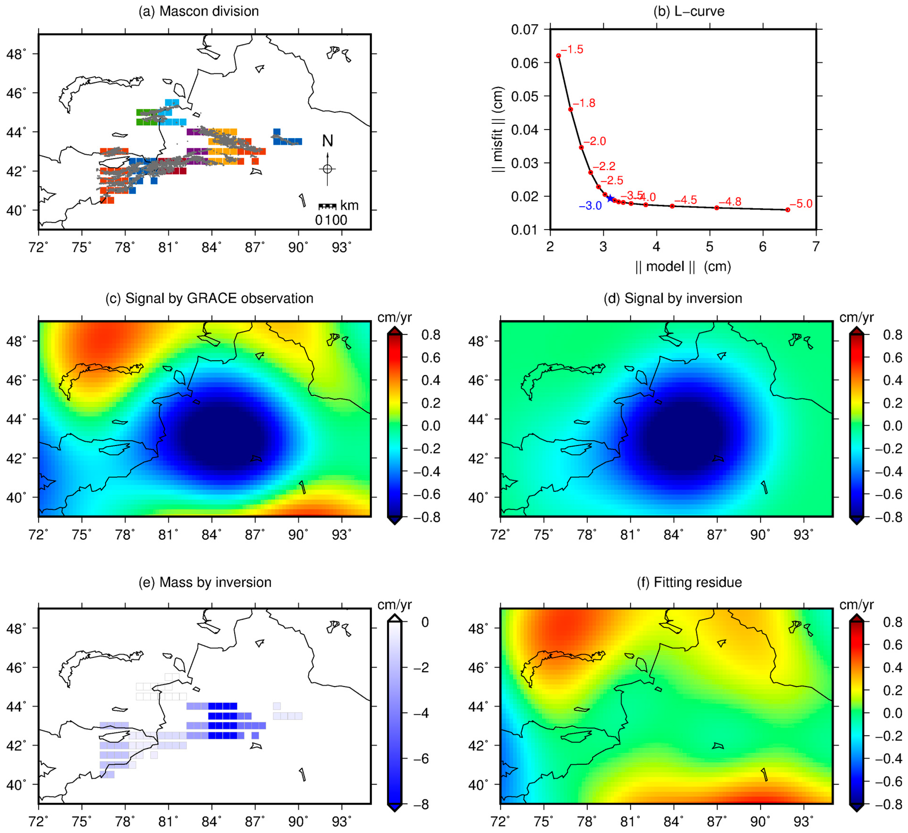
Description and Demonstration of the Inversion Method
2.2. ICESat
2.3. Lake Level Change
2.4. MODIS
2.5. Land Water Model
2.6. Precipitation
2.7. Arctic Oscillation Index (AOI)
3. Results
3.1. The Total Mass
3.2. Glaciers
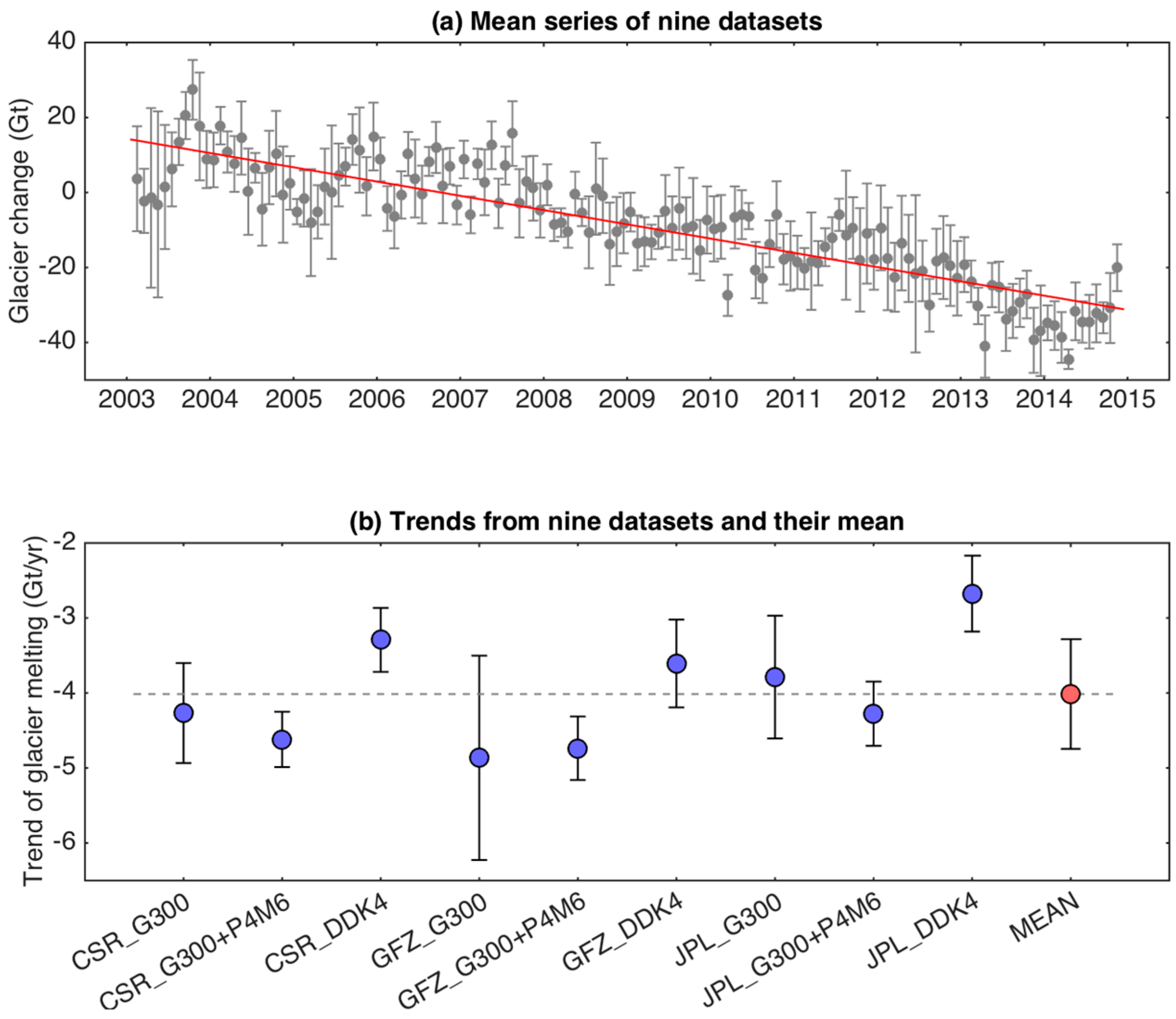
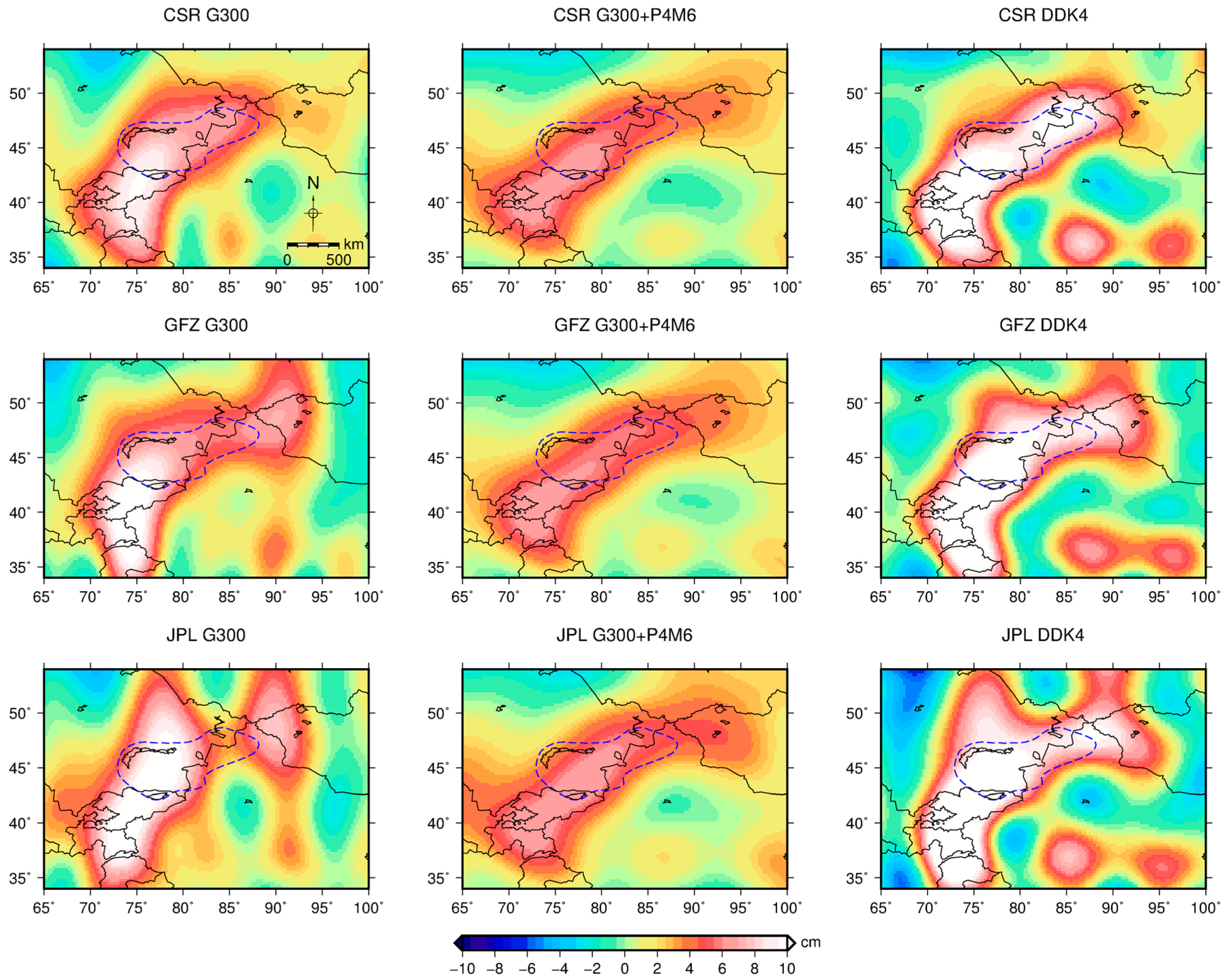
3.2.1. GRACE
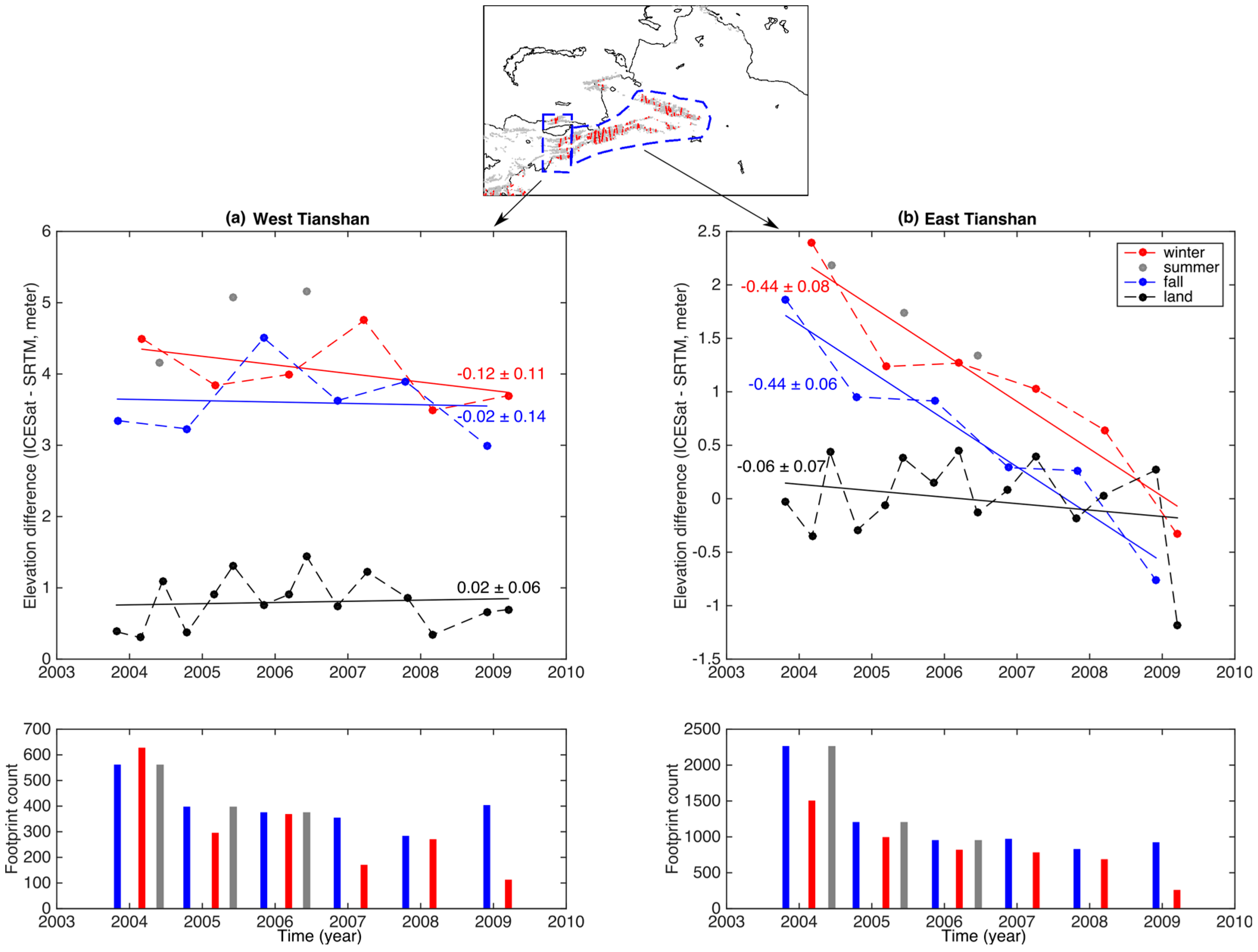
3.2.2. ICESat
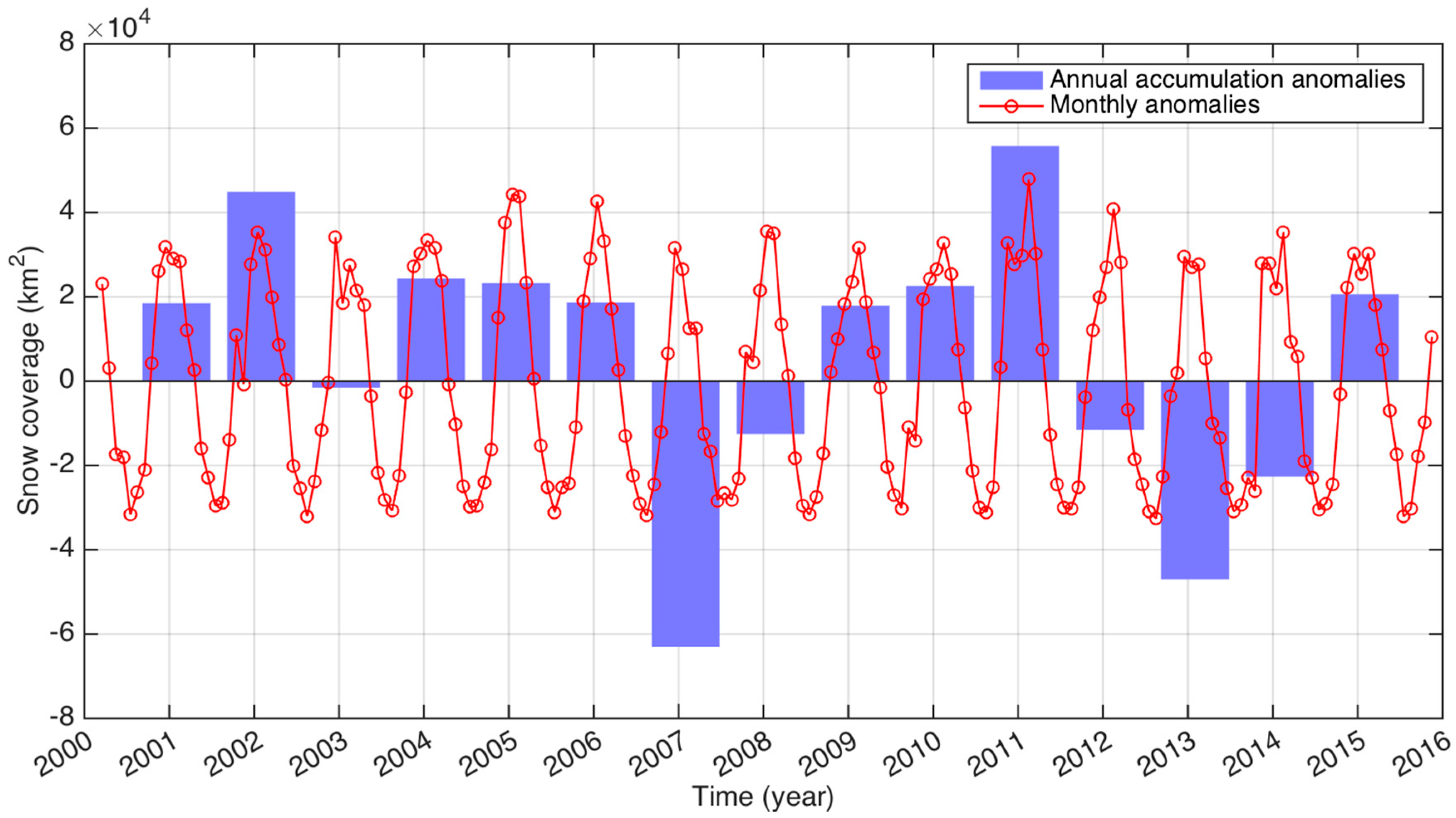
3.3. Snow Coverage
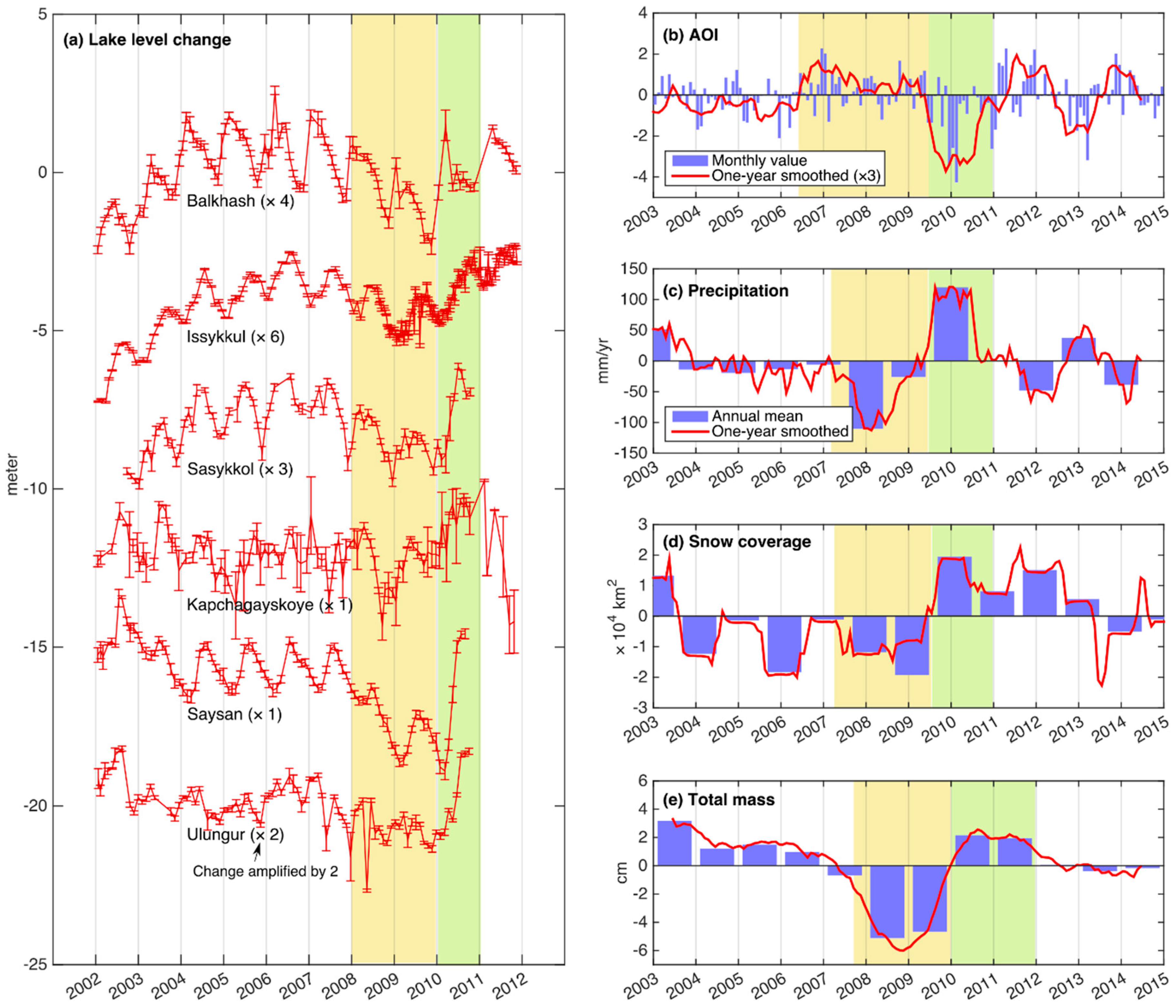
3.4. Time Series of All Factors in the Lake Area
3.5. Water Level Change in Bosten Lake over 60 Years
4. Discussion
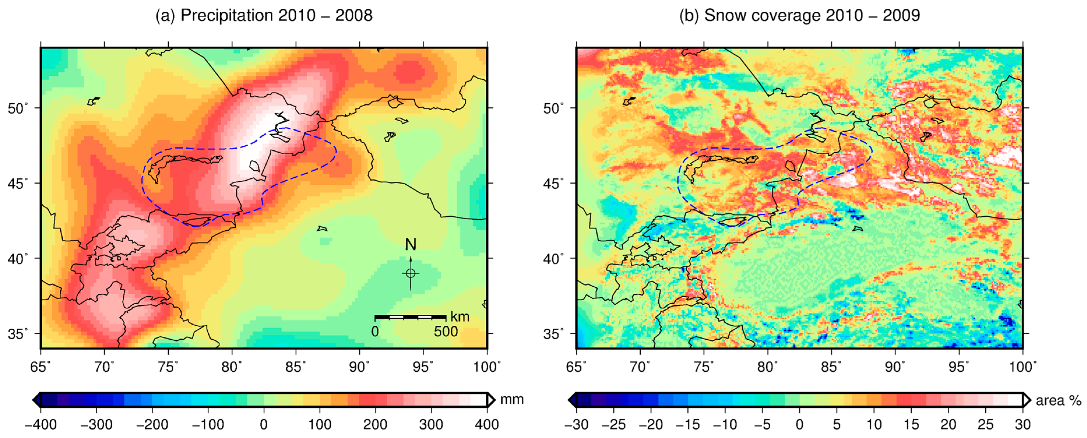
4.1. A Rapid Transition from a Dry Year (2009) to a Wet Year (2010)
4.1.1. Anomaly in the Total Mass
4.1.2. Anomalies in Precipitation and Snowfall
4.2. Water Level Change in the Bosten Lake and the Glacier Change
5. Conclusions
Acknowledgments
Author Contributions
Conflicts of Interest
Abbreviations
| GRACE | Gravity Recovery and Climate Experiment |
| MODIS | moderate-resolution imaging spectroradiometer |
| AOI | Arctic oscillation index |
| SRTM | Shuttle Radar Topography Mission |
| GLIMS | Global Land Ice Measurements from Space |
| GPCP | Global Precipitation Climatology Project |
| CSR | Center for Space Research |
| GFZ | GeoForschungsZentrum |
| JPL | Jet Propulsion Laboratory |
References
- Stocker, T.F.; Qin, D.; Plattner, G.K.; Tignor, M.; Allen, S.K.; Boschung, J.; Nauels, A.; Xia, Y.; Bex, V.; Midgley, P.M. Climate Change 2013: The Physical Science Basis; Cambridge University Press: Cambridge, UK; New York, NY, USA, 2014. [Google Scholar]
- Jacob, T.; Wahr, J.; Pfeffer, W.T.; Swenson, S. Recent contributions of glaciers and ice caps to sea level rise. Nature 2012, 482, 514–518. [Google Scholar] [CrossRef] [PubMed]
- Chen, J.L.; Wilson, C.R.; Blankenship, D.; Tapley, B.D. Accelerated antarctic ice loss from satellite gravity measurements. Nat. Geosci. 2009, 2, 859–862. [Google Scholar] [CrossRef]
- Velicogna, I.; Wahr, J. Acceleration of Greenland ice mass loss in spring 2004. Nature 2006, 443, 329–331. [Google Scholar] [CrossRef] [PubMed]
- Bolch, T.; Kulkarni, A.; Kaab, A.; Huggel, C.; Paul, F.; Cogley, J.G.; Frey, H.; Kargel, J.S.; Fujita, K.; Scheel, M.; et al. The state and fate of Himalayan glaciers. Science 2012, 336, 310–314. [Google Scholar] [CrossRef] [PubMed] [Green Version]
- Farinotti, D.; Longuevergne, L.; Moholdt, G.; Duethmann, D.; Mölg, T.; Bolch, T.; Vorogushyn, S.; Güntner, A. Substantial glacier mass loss in the tien shan over the past 50 years. Nat. Geosci. 2015. [Google Scholar] [CrossRef]
- Gardner, A.S.; Moholdt, G.; Cogley, J.G.; Wouters, B.; Arendt, A.A.; Wahr, J.; Berthier, E.; Hock, R.; Pfeffer, W.T.; Kaser, G.; et al. A reconciled estimate of glacier contributions to sea level rise: 2003 to 2009. Science 2013, 340, 852–857. [Google Scholar] [CrossRef] [PubMed] [Green Version]
- Matsuo, K.; Heki, K. Time-variable ice loss in Asian high mountains from satellite gravimetry. Earth Planet. Sci. Lett. 2010, 290, 30–36. [Google Scholar] [CrossRef]
- Yao, T.; Thompson, L.; Yang, W.; Yu, W.; Gao, Y.; Guo, X.; Yang, X.; Duan, K.; Zhao, H.; Xu, B.; et al. Different glacier status with atmospheric circulations in Tibetan Plateau and surroundings. Nat. Clim. Chang. 2012, 2, 663–667. [Google Scholar] [CrossRef]
- Immerzeel, W.W.; van Beek, L.P.; Bierkens, M.F. Climate change will affect the Asian water towers. Science 2010, 328, 1382–1385. [Google Scholar] [CrossRef] [PubMed]
- Shi, Y.; Shen, Y.; Kang, E.; Li, D.; Ding, Y.; Zhang, G.; Hu, R. Recent and future climate change in northwest China. Clim. Chang. 2006, 80, 379–393. [Google Scholar] [CrossRef]
- Bolch, T.; Buchroithner, M.; Pieczonka, T.; Kunert, A. Planimetric and volumetric glacier changes in the Khumbu Himal, Nepal, since 1962 using Corona, Landsat TM and ASTER data. J. Glaciol. 2008, 54, 592–600. [Google Scholar] [CrossRef]
- Andreassen, L.M.; Paul, F.; Kääb, A.; Hausberg, J.E. Landsat-derived glacier inventory for Jotunheimen, Norway, and deduced glacier changes since the 1930s. Cryosphere 2008, 2, 131–145. [Google Scholar] [CrossRef] [Green Version]
- Gardelle, J.; Berthier, E.; Arnaud, Y. Slight mass gain of Karakoram glaciers in the early twenty-first century. Nat. Geosci. 2012, 5, 322–325. [Google Scholar] [CrossRef]
- Gardelle, J.; Berthier, E.; Arnaud, Y.; Kääb, A. Region-wide glacier mass balances over the Pamir-Karakoram-Himalaya during 1999–2011. Cryosphere 2013, 7, 1263–1286. [Google Scholar] [CrossRef] [Green Version]
- Kääb, A.; Berthier, E.; Nuth, C.; Gardelle, J.; Arnaud, Y. Contrasting patterns of early twenty-first-century glacier mass change in the Himalayas. Nature 2012, 488, 495–498. [Google Scholar] [CrossRef] [PubMed]
- Bolch, T.; Sørensen, L.S.; Simonssen, S.B.; Mölg, N.; Machguth, H.; Rastner, P.; Paul, F. Mass loss of Greenland’s glaciers and ice caps 2003–2008 revealed from ICESat laser altimetry data. Geophys. Res. Lett. 2013, 40, 875–881. [Google Scholar] [CrossRef] [Green Version]
- Neckel, N.; Kropáček, J.; Bolch, T.; Hochschild, V. Glacier mass changes on the Tibetan Plateau 2003–2009 derived from ICESat laser altimetry measurements. Environ. Res. Lett. 2014, 9, 014009. [Google Scholar] [CrossRef]
- Yi, S.; Sun, W. Evaluation of glacier changes in high-mountain Asia based on 10 year grace rl05 models. J. Geophys. Res. Solid Earth 2014, 119, 2504–2517. [Google Scholar] [CrossRef]
- Tapley, B.D.; Bettadpur, S.; Ries, J.C.; Thompson, P.F.; Watkins, M.M. Grace measurements of mass variability in the earth system. Science 2004, 305, 503–505. [Google Scholar] [CrossRef] [PubMed]
- Yi, S.; Wang, Q.; Sun, W. Basin mass dynamic changes in China from GRACE based on a multibasin inversion method. J. Geophys. Res. Solid Earth 2016, 121. [Google Scholar] [CrossRef]
- Yi, S.; Sun, W. Characteristics of gravity signal and loading effect in China. Geod. Geodyn. 2015, 6, 280–285. [Google Scholar] [CrossRef]
- Zhao, Q.; Wu, W.; Wu, Y. Variations in China’s terrestrial water storage over the past decade using grace data. Geod. Geodyn. 2015, 6, 187–193. [Google Scholar] [CrossRef]
- Yi, S.; Sun, W.; Heki, K.; Qian, A. An increase in the rate of global mean sea level rise since 2010. Geophys. Res. Lett. 2015, 42, 3998–4006. [Google Scholar] [CrossRef]
- Chen, J.; Wilson, C.; Tapley, B. Contribution of ice sheet and mountain glacier melt to recent sea level rise. Nat. Geosci. 2013, 6, 549–552. [Google Scholar] [CrossRef]
- Barthelmes, F.; Köhler, W. International Centre for Global Earth Models (ICGEM). J. Geod. 2012, 86, 932–934. [Google Scholar]
- Swenson, S.; Chambers, D.; Wahr, J. Estimating geocenter variations from a combination of grace and ocean model output. J. Geophys. Res. Solid Earth (1978–2012) 2008, 113. [Google Scholar] [CrossRef]
- Cheng, M.; Ries, J.C.; Tapley, B.D. Variations of the Earth’s figure axis from satellite laser ranging and GRACE. J. Geophys. Res. Solid Earth (1978–2012) 2011, 116. [Google Scholar] [CrossRef]
- Wahr, J.; Molenaar, M.; Bryan, F. Time variability of the Earth’s gravity field: Hydrological and oceanic effects and their possible detection using GRACE. J. Geophys. Res. Solid Earth 1998, 103, 30205–30229. [Google Scholar] [CrossRef]
- Swenson, S.; Wahr, J. Post-processing removal of correlated errors in GRACE data. Geophys. Res. Lett. 2006, 33. [Google Scholar] [CrossRef]
- Kusche, J.; Schmidt, R.; Petrovic, S.; Rietbroek, R. Decorrelated GRACE time-variable gravity solutions by GFZ, and their validation using a hydrological model. J. Geod. 2009, 83, 903–913. [Google Scholar] [CrossRef]
- Hansen, P.C.; O’Leary, D.P. The use of the L-curve in the regularization of discrete ill-posed problems. SIAM J. Sci. Comput. 1993, 14, 1487–1503. [Google Scholar] [CrossRef]
- GLIMS: Global Land Ice Measurements from Space. Available online: http://www.glims.org/glimsblurb.html (accessed on 21 September 2016).
- Farr, T.G.; Rosen, P.A.; Caro, E.; Crippen, R.; Duren, R.; Hensley, S.; Kobrick, M.; Paller, M.; Rodriguez, E.; Roth, L.; et al. The shuttle radar topography mission. Rev. Geophys. 2007, 45. [Google Scholar] [CrossRef]
- Huss, M. Density assumptions for converting geodetic glacier volume change to mass change. Cryosphere 2013, 7, 877–887. [Google Scholar] [CrossRef]
- Global Reservoirs/Lakes (G-REALM). Available online: http://www.pecad.fas.usda.gov/cropexplorer/global_reservoir/ (accessed on 21 September 2016).
- Crétaux, J.-F.; Jelinski, W.; Calmant, S.; Kouraev, A.; Vuglinski, V.; Bergé-Nguyen, M.; Gennero, M.-C.; Nino, F.; Rio, R.A.D.; Cazenave, A.; et al. SOLS: A lake database to monitor in the Near Real Time water level and storage variations from remote sensing data. Adv. Space Res. 2011, 47, 1497–1507. [Google Scholar] [CrossRef]
- Hall, D.; Salomonson, V.; Riggs, G. Modis/Terra Snow Cover Daily l3 Global 500 m Grid, 5th ed.; National Snow and Ice Data Center: Boulder, CO, USA, 2006. [Google Scholar]
- MODIS/Terra Snow Cover Monthly L3 Global 0.05Deg CMG, Version 6. Available online: http://nsidc.org/data/MOD10CM (accessed on 21 September 2016).
- Rodell, M.; Houser, P.R.; Jambor, U.; Gottschalck, J.; Mitchell, K.; Meng, C.J.; Arsenault, K.; Cosgrove, B.; Radakovich, J.; Bosilovich, M.; et al. The global land data assimilation system. Bull. Am. Meteorol. Soc. 2004, 85. [Google Scholar] [CrossRef]
- Adler, R.F.; Huffman, G.J.; Chang, A.; Ferraro, R.; Xie, P.P.; Janowiak, J.; Rudolf, B.; Schneider, U.; Curtis, S.; Bolvin, D.; et al. The version-2 global precipitation climatology project (GPCP) monthly precipitation analysis (1979-present). J. Hydrometeorol. 2003, 4, 1147–1167. [Google Scholar] [CrossRef]
- PSD Gridded Climate Datasets: Precipitation. Available online: http://www.esrl.noaa.gov/psd/data/gridded/tables/precipitation.html (accessed on 21 September 2016).
- Thompson, D.W.; Wallace, J.M. The arctic oscillation signature in the wintertime geopotential height and temperature fields. Geophys. Res. Lett. 1998, 25, 1297–1300. [Google Scholar] [CrossRef]
- Daily Arctic Oscillation Index. Available online: http://www.cpc.ncep.noaa.gov/products/precip/CWlink/daily_ao_index/ao_index.html (accessed on 21 September 2016).
- Li, Y.-A.; Tan, Y.; Jiang, F. Study on Hydrological Features of the Kaidu River and the Bosten Lake in the Second Half of 20th Century. J. Glaciol. Geocryol. 2003, 25, 215–218. [Google Scholar]
- Sun, Z.; Wang, R.; Huang, Q. Comparison of water level changes during the past 20 years between Daihai and Bositen Lakes. J. Arid Land Resour. Environ. 2006, 20, 56–60. [Google Scholar]
- Qiu, H.; Zhao, Q.; Zhu, W.; Tao, R.; Qian, H. Analysis of the Bosten lake’s level and its possible mechanism. J. Meteorol. Sci. 2013, 33, 289–295. [Google Scholar]
- Wang, X.; Gong, P.; Zhao, Y.; Xu, Y.; Cheng, X.; Niu, Z.; Luo, Z.; Huang, H.; Sun, F.; Li, X. Water-level changes in China’s large lakes determined from ICESat/GLAS data. Remote Sens. Environ. 2013, 132, 131–144. [Google Scholar] [CrossRef]
- Saving Bosten Lake. Available online: http://news.ts.cn/content/2014-04/14/content_9549017_all.htm (accessed on 21 September 2016). (In Chinese)
- Wang, J.; Chen, Y.-N.; Chen, Z.-S. Quantitative assessment of climate change and human activities impact the inflowing runoff of Bosten Lake. Xinjiang Agric. Sci. 2012, 49, 581–587. [Google Scholar]


| Region | Number of Glaciers | Area (km2) | Mean Elevation (m) |
|---|---|---|---|
| 1 | 360 | 150.82 | 3750 |
| 2 | 1000 | 304.03 | 4015 |
| 3 | 2426 | 1568.11 | 4015 |
| 4 | 1045 | 584.23 | 3829 |
| 5 | 73 | 34.54 | 3671 |
| 6 | 271 | 111.17 | 3754 |
| 7 | 1809 | 3475.32 | 4109 |
| 8 | 1350 | 3146.3 | 4402 |
| 9 | 2033 | 1608.6 | 4310 |
| Data | Time Period | Spatial Resolution | Target | Annotation |
|---|---|---|---|---|
| GRACE | 2003–2014 | ~300 km | Total mass and glaciers | Inversion method is adopted to estimate the total mass change in the central Tianshan. |
| ICESat | 2003–2009 | 70 m | Glaciers | Mean elevation is obtained to estimate the total mass change in the central Tianshan. |
| Altimetry | 2002–2010/2011 | Several kilometers | Lake level | Lake level record of the Bosten Lake is extended by site observations. |
| MODIS | 2000–2015 | 0.05° | Snow coverage | Only fraction of coverage is available. |
| GLDAS | 2003–2014 | 1° | Soil moisture and snow volume | There are four models. |
| GPCP | 2003–2014 | 2.5° | Precipitation | The dataset is interpolated to a finer resolution of 1° × 1°. |
| AOI | 1950–2014 | N/A | Westerlies | AOI is an indicator of the westerlies. |
© 2016 by the authors; licensee MDPI, Basel, Switzerland. This article is an open access article distributed under the terms and conditions of the Creative Commons Attribution (CC-BY) license (http://creativecommons.org/licenses/by/4.0/).
Share and Cite
Yi, S.; Wang, Q.; Chang, L.; Sun, W. Changes in Mountain Glaciers, Lake Levels, and Snow Coverage in the Tianshan Monitored by GRACE, ICESat, Altimetry, and MODIS. Remote Sens. 2016, 8, 798. https://doi.org/10.3390/rs8100798
Yi S, Wang Q, Chang L, Sun W. Changes in Mountain Glaciers, Lake Levels, and Snow Coverage in the Tianshan Monitored by GRACE, ICESat, Altimetry, and MODIS. Remote Sensing. 2016; 8(10):798. https://doi.org/10.3390/rs8100798
Chicago/Turabian StyleYi, Shuang, Qiuyu Wang, Le Chang, and Wenke Sun. 2016. "Changes in Mountain Glaciers, Lake Levels, and Snow Coverage in the Tianshan Monitored by GRACE, ICESat, Altimetry, and MODIS" Remote Sensing 8, no. 10: 798. https://doi.org/10.3390/rs8100798