Testing a Modified PCA-Based Sharpening Approach for Image Fusion

Abstract

Image data sharpening is a challenging field of remote sensing science, which has become more relevant as high spatial-resolution satellites and superspectral sensors have emerged. Although the spectral property is crucial for mineral mapping, spatial resolution is also important as it allows targeted minerals/rocks to be identified/interpreted in a spatial context. Therefore, improving the spatial context, while keeping the spectral property provided by the superspectral sensor, would bring great benefits for geological/mineralogical mapping especially in arid environments. In this paper, a new concept was tested using superspectral data (ASTER) and high spatial-resolution panchromatic data (WorldView-2) for image fusion. A modified Principal Component Analysis (PCA)-based sharpening method, which implements a histogram matching workflow that takes into account the real distribution of values, was employed to test whether the substitution of Principal Components (PC1–PC4) can bring a fused image which is spectrally more accurate. The new approach was compared to those most widely used—PCA sharpening and Gram–Schmidt sharpening (GS), both available in ENVI software (Version 5.2 and lower) as well as to the standard approach—sharpening Landsat 8 multispectral bands (MUL) using its own panchromatic (PAN) band. The visual assessment and the spectral quality indicators proved that the spectral performance of the proposed sharpening approach employing PC1 and PC2 improve the performance of the PCA algorithm, moreover, comparable or better results are achieved compared to the GS method. It was shown that, when using the PC1, the visible-near infrared (VNIR) part of the spectrum was preserved better, however, if the PC2 was used, the short-wave infrared (SWIR) part was preserved better. Furthermore, this approach improved the output spectral quality when fusing image data from different sensors (e.g., ASTER and WorldView-2) while keeping the proper albedo scaling when substituting the second PC.

1. Introduction

Image data sharpening is a challenging field of remote sensing science, which became more popular after the recent emergence of high spatial resolution satellite image sensors. These satellites usually provide one broad panchromatic (PAN) band with a high spatial resolution and multispectral (MUL) images at a coarser spatial resolution. The general approach is to use the PAN band to enhance the spatial resolution of the multispectral images using sharpening methods, which use different algorithms to inject the spatial detail of the PAN image to the higher spectral resolution image data. An ideal sharpening algorithm should improve both spatial and spectral information in the fused image. To simultaneously keep both spatial and spectral performance at a good level is still rather challenging, thus research leading to the development of pansharpening algorithms is still topical. The main problems observed are deviations in the spatial accuracy and in the spectral values of the sharpened image [1]. These are still the key issues that need to be solved prior to employing classifications to the sharpened image.

Generally, sharpening algorithms can be divided by several means (e.g., [2,3,4,5,6,7]). The first group can be described as component substitution algorithms (CS). The most prominent algorithms of this group are Principal component analysis (PCA), Intensity–hue–saturation (IHS), Gram–Schmidt transform (GS), Ehlers fusion (EF) or Brovey transform (BT). These algorithms have the advantage of low computing time, easy implementation and great visual interpretive quality, although the spectral accuracy may be not sufficient enough [8], thus being an issue for most remote sensing applications based on spectral signatures [9]. Improvement of the spectral accuracy in the sharpened images was gained by algorithms based on decimated wavelet transform (DWT) or Laplacian pyramid transform (LP). These algorithms form the second group of sharpening methods, usually called the multi-resolution analysis (MRA) approach [10]. The general principle behind MRA algorithms is usage of multiresolution decomposition, which extracts details from PAN band. Spatial information is then injected into resampled MS bands [11]. As described in [3], multi-resolution analysis approaches are good in preserving spectral information but, on the other hand, they are not able to preserve object contours and general spatial smoothness. Therefore, several improvements in the wavelet transform, which can reduce the artifacts caused by the DWT, have been introduced, such as Undecimated DWT or Non-subsampled contourlet transform (NSCT) [7,12]. Moreover, besides the MRA techniques, new approaches such as compressed sensing approaches have been successfully employed, allowing the preservation of spectral and spatial information [13,14].

In both groups of algorithms several constraints have been reported, which limit the selection of a sharpening algorithm when sharpening superspectral satellite data with a relatively coarse spatial resolution (15–30 m) using a very high-spatial resolution panchromatic band from a different sensor (e.g., WorldView-2 or -3, pixel size: 0.5 m). Most of the multi-resolution algorithms are appropriate for cases where the resolution ratio between the MUL and PAN bands is a power of two [2] and usually up to 1:6 [11]. In addition some of the CS algorithms, such as IHS in its original form, can work with just three spectral bands [15,16]. This issue is becoming extremely relevant when the new-generation superspectral satellite—Sentinel 2—was launched in June 2015, and, moreover, when the new hyperspectral satellites will be operating in orbit in the near future (e.g., EnMAP from 2018).

Although spectral property is crucial for mineral mapping, spatial resolution is also important as it allows targeted minerals/rocks to be identified/interpreted in a spatial context. Therefore, improving the spatial context, while keeping the spectral property provided by the superspectral sensor, would bring great benefits for geological/mineralogical mapping especially in arid environments.

In this paper, a new concept using superspectral data (ASTER image data providing the nine optical bands within the visible, near and shortwave infrared spectral regions) and high spatial-resolution panchromatic data (PAN band, WolrdView-2) for image fusion was tested. An area covering 27 km² and located in western Mongolia, characterized by an arid environment, was selected for the test site. High differences in the spatial resolution between these two types of satellite data (PAN band: 0.5-m vs. 15- and 30-m, respectively) as well as in the spectral property (PAN broad band covering 0.45–0.80 μm vs. nine ASTER optical bands covering 0.52–2.43 μm) are still the main constraints. There are still a limited number of studies using this type of data for image fusion [17].

As has already been mentioned, CS algorithms are popular mainly because of their easy implementation, their availability in most popular software and their low computational time. Algorithms of the CS group, such as the PCA-based approach, are among the most-widely used, they are also designed to produce very good visual results characterized by sharp edges and well preserved spatial features. To improve the performance of the CS algorithms, PCA and MRA approaches have been combined together and new methods have been employed, such as Adaptive PCA (APCA) [18], PCA with a multiresolution wavelet decomposition (MWD) [7,19], a hybrid method that combines PCA and contourlet transform methods [18,20] and non-linear variants of PCA, such as the Kernel PCA (KPCA) [21].

To keep the spectral information on geological properties provided by ASTER while improving the spatial content, the PCA-based sharpening approach was adopted and further modified and a new histogram matching concept was implemented. For a comparison, the same processing was also employed to the Landsat 8 dataset. In this case, the LANDSAT 8 panchromatic (PAN) band is used to sharpen the multispectral optical bands, thus this approach represents simpler, and to some extent a more standard, sharpening example. The results of image fusion were validated using visual inspection as well as diverse quantitative metrics (consistency and synthesis assessment). Furthermore, the spectral quality between the original pixel reflectance spectra and the corresponding spectra was assessed using four different surface targets.

2. Satellite Data Used for Sharpening/Fusion

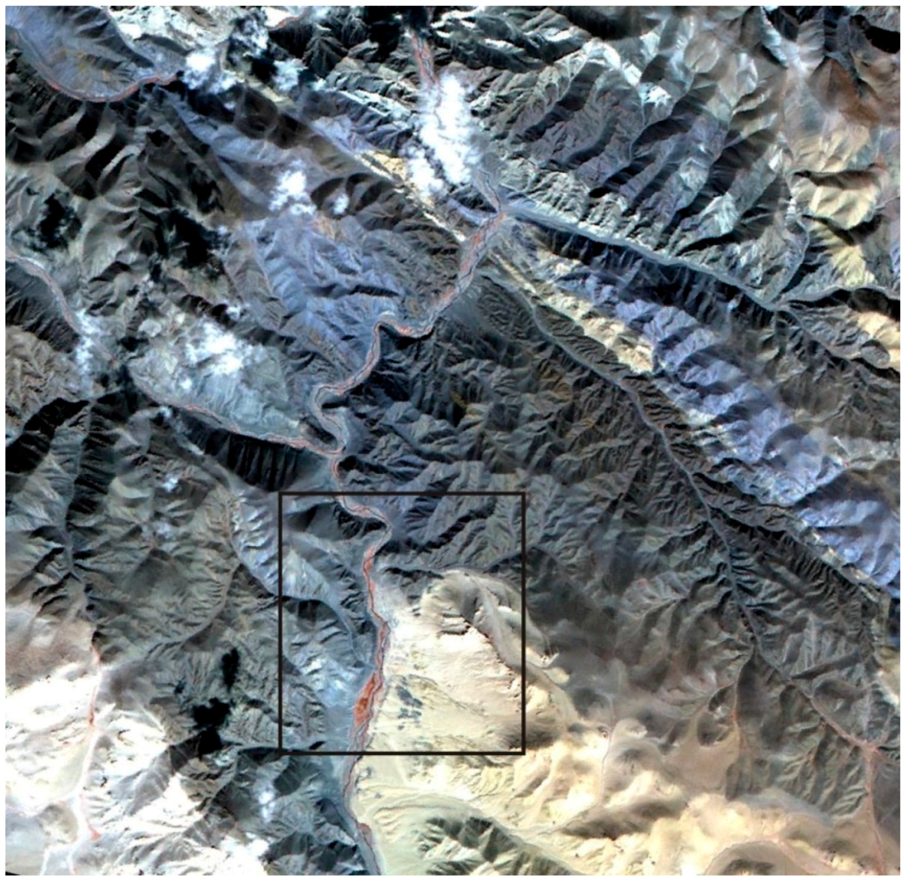
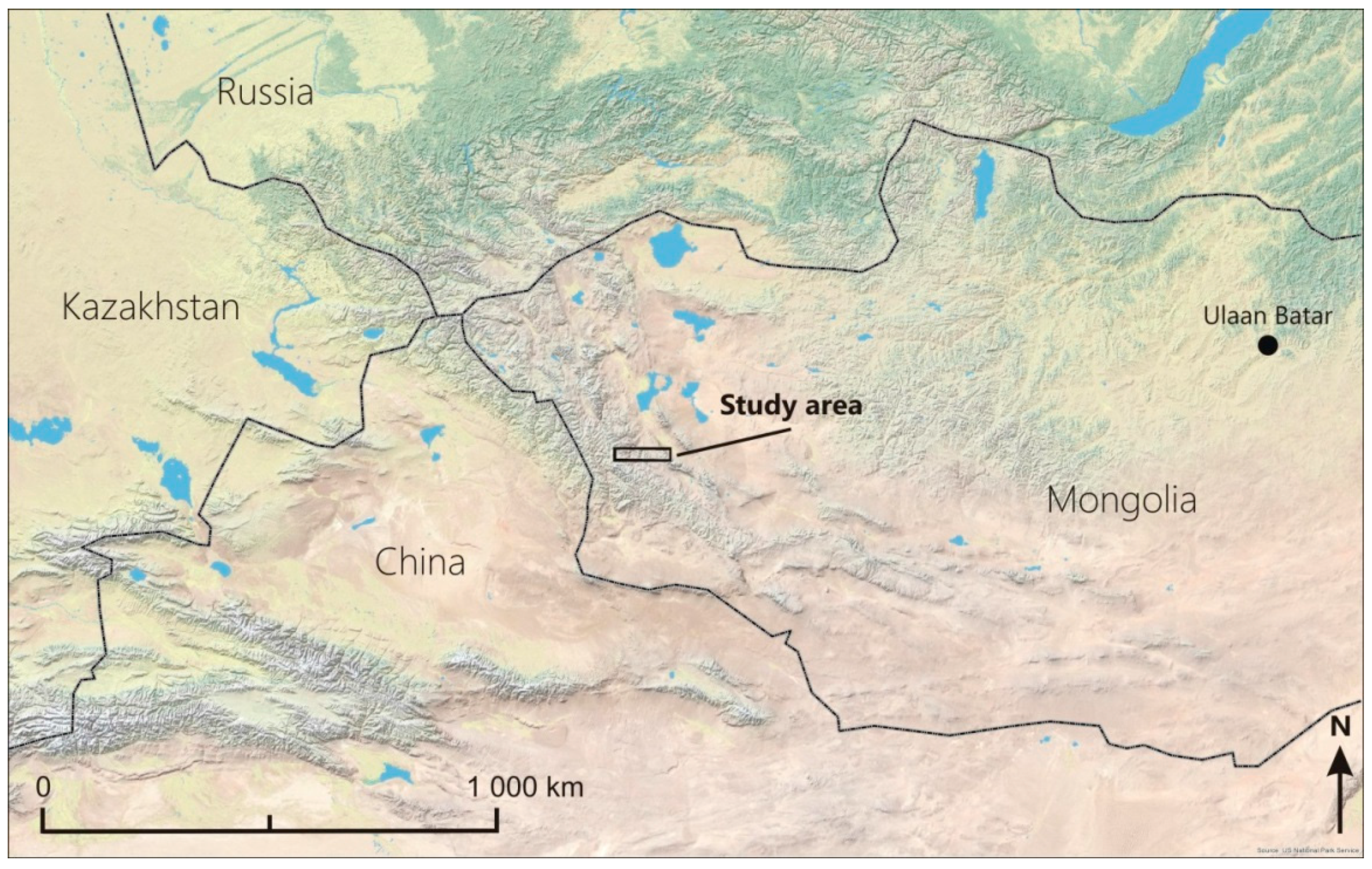
The primary remote sensing objective was to produce mineral maps for the areas of interest. To support geological mapping in the Khovd Province, western Mongolia (Figure 1), data from two different platforms/instruments, ASTER (Terra satellite) and WorldView-2, were utilized. The ASTER data provides several bands in the short wave infrared (SWIR) spectral region and therefore has a great potential for geological and mineral mapping. However, the spatial resolution is rather coarse for geological mapping at a 1:25,000 scale. The WorldView-2 data are provided at one of the highest spatial resolutions available nowadays. The spatial and spectral fusion of both datasets potentially brings significant benefits to the remote sensing applications in geology, because it would allow combining ASTER’s strong spectral and WorldView’s strong spatial aspects.

The specifications of the satellite datasets used in the presented study are summarized in

Table 1. Technical specifications of image datasets used in the study.

Sensor Name	Band Name	Spectral Range (μm)	Resolution (m)	Date/Hour of Acquisition
Landsat 8	B1	0.43–0.45	30	30 August 2013, 04:44:49
	B2	0.45–0.51	30	30 August 2013, 04:44:49
	B3	0.53–0.59	30	30 August 2013, 04:44:49
	B4	0.64–0.67	30	30 August 2013, 04:44:49
	B5	0.85–0.88	30	30 August 2013, 04:44:49
	B6	1.57–1.65	30	30 August 2013, 04:44:49
	B7	2.11–2.29	30	30 August 2013, 04:44:49
	PAN	0.50–0.68	15	30 August 2013, 04:44:49
ASTER	B1	0.52–0.6	15	3 October 2005, 04:59:17
	B2	0.63–0.69	15	3 October 2005, 04:59:17
	B3	0.76–0.86	15	3 October 2005, 04:59:17
	B5	1.6–1.7	30	3 October 2005, 04:59:17
	B6	2.145–2.185	30	3 October 2005, 04:59:17
	B7	2.185–2.225	30	3 October 2005, 04:59:17
	B8	2.235–2.285	30	3 October 2005, 04:59:17
	B9	2.295–2.365	30	3 October 2005, 04:59:17
	B10	2.36–2.43	30	3 October 2005, 04:59:17
WorldView-2	PAN	0.45–0.8	0.5	22 March 2012, 05:04:16

. The ASTER (Figure 2) dataset consists of 9 optical bands with a spatial resolution from 15 (VNIR) to 30 m (SWIR). The data were acquired on 3 March 2005 and were provided by Japan Space Systems. The ASTER data were orthorectified and converted to reflectance values using ENVI and ATCOR 2 software. The orthorectified WV2 data were acquired on 22 March 2012 and were provided by Digital Globe, Inc. (Westminster, CO, USA).

To compare the results of the image fusion (ASTER MUL and WV2 PAN), the Landsat 8 MUL data (Table 1) acquired on 30 August 2013 were sharpened using its own PAN band, as this approach represents a standard image sharpening example. Considering the Landsat 8 multispectral bands, the surface reflectance product provided by NASA [22] was further used in this study. Cirrus and TIR bands were excluded from the Landsat 8 dataset prior to any sharpening analysis.

3. Methods

3.1. Regular PCA Sharpening Method

One of the most used methods of pansharpening is Principal component analysis (PCA). The method was originally introduced as a general statistical method for linear decorrelation of the input dataset [23]. Data entering the algorithm are decomposed into the new coordinate system described by eigenvectors, using the orthogonal affine transform, where the first axis is in the direction of the highest variance of the original dataset [24]. Subsequent axes are in the direction of the second, third, etc. largest variation of the original dataset. All axes are perpendicular to each other in the new coordinate system. Each principal component (PC) has assigned a score and a transformation weight. There can be as many PCs as there are multispectral bands in the image data set; however, the first PCs (usually first three PCs), account for the greatest variability in the data [25].

In the pansharpening perspective, PCA is performed to compress the spectral information of the MS data into a couple of principle component bands (PCs). During the transformation the spatial content of the original data is projected into the 1st PC, while most of the spectral information from all the bands is transformed into other PCs besides the first one [7]. This is why the 1st PC is usually chosen as the target for PAN substitution and the 1st PC is then resampled to a high spatial resolution of the PAN band. Before injecting the high spatial-resolution PAN band, it is necessary to match the histograms of the injected PAN band and the 1st PC that is to be substituted. The inverse PCA is performed in the last step of the sharpening process, resulting in the sharpened image. PCA, as a very simple non-parametric technique, has numerous disadvantages, such as weak spectral output. On the other hand, its strength lies in the spatial domain [7].

3.2. Proposed Modifications for Image Fusion

In this study, the PCA method was adopted mainly because of its broad availability throughout the remote sensing software (SW). By default, software (SW), such as ENVI or Erdas Imagine, uses only the 1st PC in the sharpening process. Users cannot manually edit parameters of the sharpening algorithm, such as selection of the principal component to be substituted or the histogram matching techniques. This makes the sharpening process inflexible for a wide variety of applications and input data and may not be optimal if mineral spectral mapping is demanded, as the 1st PC contains not only the spatial information, but also an albedo component which is connected to the spectral information in other PCs. Therefore, in the standard PCA sharpening process, when the 1st PC is substituted, most of the albedo information is lost and the missing albedo information may cause spectral shifts and biases in the resulting sharpened image when the inverse PCA is employed.

Therefore, the intention was to test if the PC of a higher order (e.g., PC2) will lead to better preservation of the spectral information via the sharpening process. The first four principal components (PC1–PC4) were used to compress the spectral information and were consequently spatially sharpened using the PAN band. It was expected that the first two PCs have the potential to give good results when employing the PCA sharpening process, however PC3 and PC4 were used to compare the result and explain it in a wider context.

Another crucial step of the PCA sharpening method is histogram matching. Histogram matching between the injected PAN band and the substituting PC directly affects the results of the consequent PCA inversion transformation. Coefficients of the covariance matrix, which are crucial for the inverse PCA, would cause an incorrect transformation to the image values if the distribution of the values in the high spatial resolution image is different from those of the desired principal component (PC). As already mentioned, in the available software, the PCA algorithms are mostly “black boxes” and users are not able to find out how the histogram matching proceeds, neither is it possible to get information about possible additional histogram stretching, which may be applied to the resulting images.

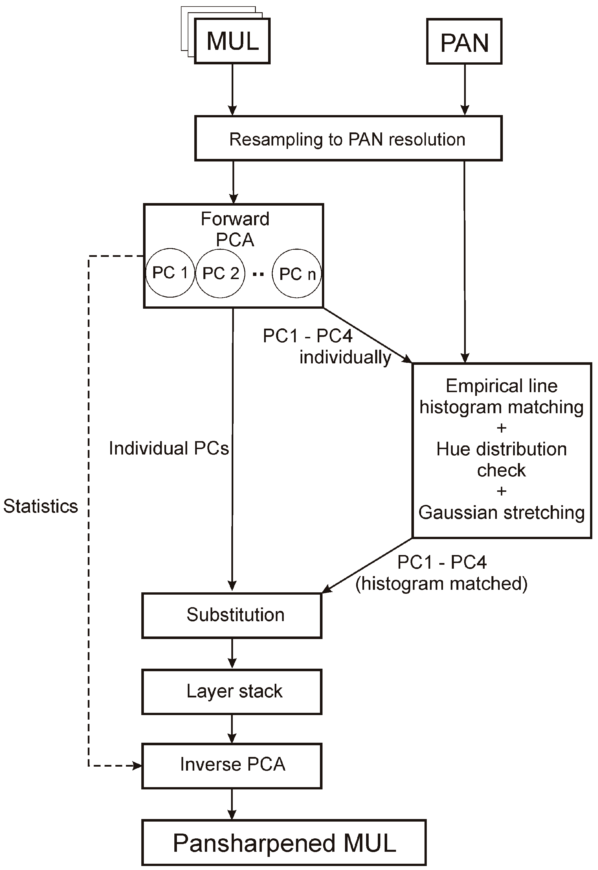
In this study, a new histogram matching workflow, which takes into account the real distribution of values in the images, was developed. The range of values was measured using the Empirical line method (Equation (1)), which allows automatic identification of the brightest and darkest points within an image, in this case the PCs used for the substitution. The Empirical line method is usually used for radiometric corrections of image data, where it calculates the empirical relation between radiance and reflectance and is defined by the equation [26]:

L = gain × DN + offset,

(1)

where L is relative reflectance and DN is a digital number.

The method represents the general approach for histogram recalculations from the input range to the new range. For the purposes of this study, Equation (2) for the Empirical line method is described as:

NewPANvalue = gain × PANvalue + offset,

(2)

where gain and offset are variables which are calculated from the darkest and brightest pixel-pairs values in both PAN and each PC bands. The resulting range is applied to the matched image, a high spatial resolution panchromatic band, and all the image values are then recalculated using a linear line constructed between the brightest and darkest points.

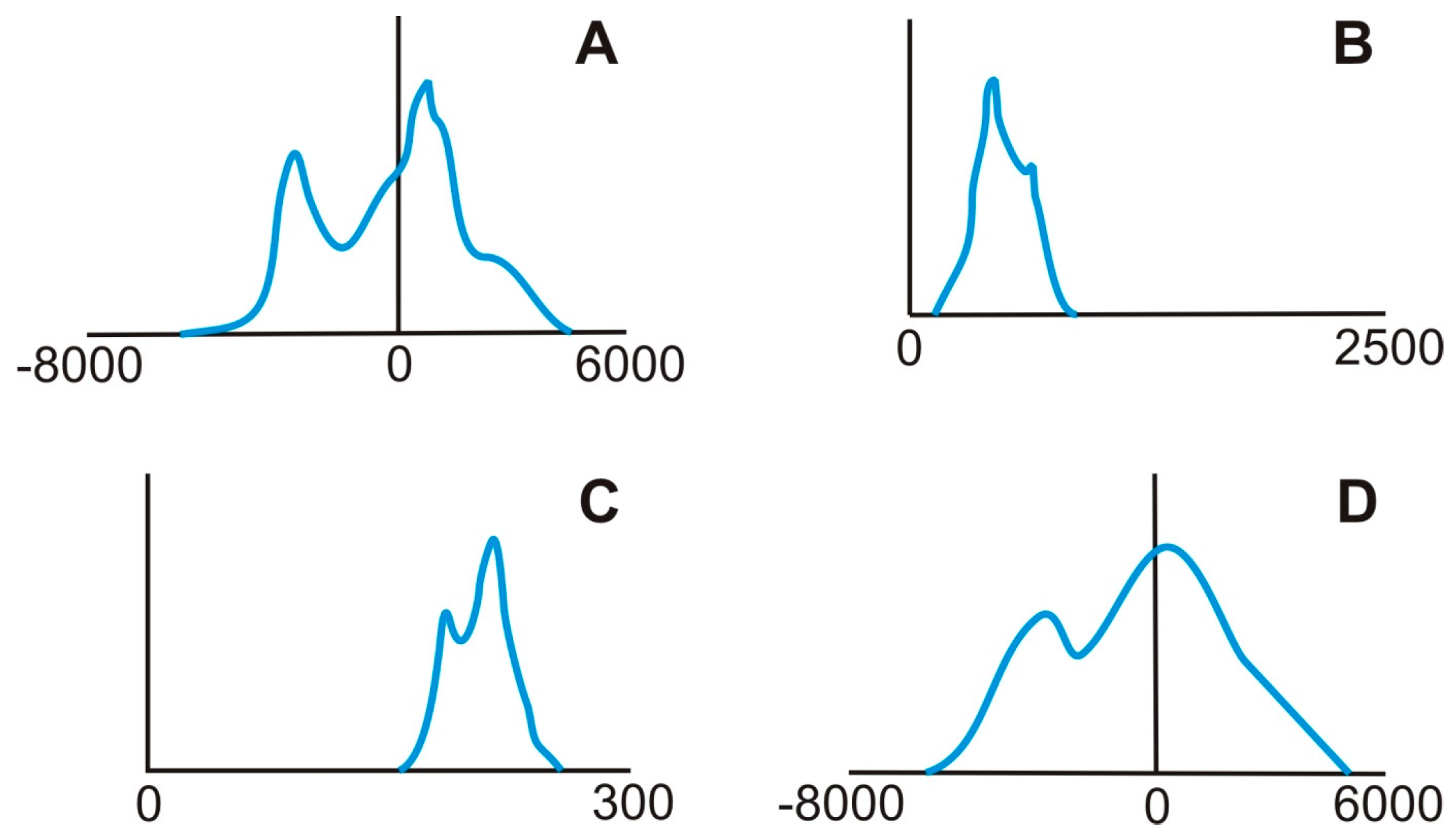
The relative distances of all the pixel values from the line are maintained and are used as a mean for the recalculation. The best result can be achieved via an inversion when the histogram matched image has the most similar range of values with the original PC. After employing histogram matching using the Empirical line, the histogram usually has the same distribution, but does not have the same range of values. In order to solve this problem, Gaussian histogram stretching was applied after histogram matching (Figure 3).

3.3. Data Processing

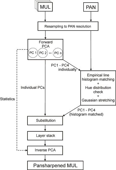
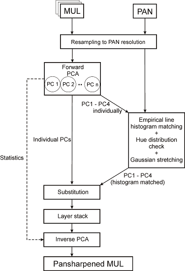
The modified PCA sharpening method (Figure 4) described above was employed to the ASTER dataset while the WorldView-2 PAN band was used to sharpen the ASTER MUL bands. The spatial resolution of the WorldView-2 PAN band is 0.5 m, while the spatial resolution of the ASTER image is 15-m (VNIR) and 30-m (SWIR), respectively. The difference in the spatial resolutions of the two image data sets is much higher than recommended in the literature [2]. In order to test the effect of different ratios between the spatial resolutions of the two fused image data sets, the original ASTER data were sharpened not only to a 0.5-m resolution (the original spatial resolution of the WV2 PAN band), but also to a 3.0-m spatial resolution. For both scenarios, four sharpened images were computed, when the first four PCs were substituted by the histogram-matched PAN band (resampled to either 0.5-m or 3.0-m using the nearest neighbor method (NN)).

In order to test the modified PCA approach on a standard dataset, the same workflow employed on the ASTER dataset was employed on the Landsat 8 dataset. Landsat 8 has a ratio between PAN and MUL of 1:2, which is more suitable for the sharpening process. Both PAN (15-m spatial resolution) and MUL (30-m spatial resolution) are acquired at the same time from the same platform which minimizes spatial distortions caused by spatial miss-registration during the sharpening process. For a comparison, the sharpening was also employed using the built-in PCA algorithm (ENVI PCA sharpening method) as well as the Gram–Schmidt sharpening (ENVI GS sharpening method) method, both built-in tools available in the ENVI software.

3.4. Validation

All sharpening algorithms introduce some degree of spatial and spectral distortion into the sharpened image. Therefore, it is necessary to test the proposed adjustments to the PCA sharpening method using objective metrics for spectral/spatial quality. A visual comparison is often used as the first spatial quality metrics. Several image global quality features, like artifacts, linear features, edges, textures, colors, blurring or blooming can be observed and assessed using visual inspection [7]. Therefore, the results of PC1–PC4 substitution and the new histogram matching scheme were visually assessed at first.

Spectral consistency, unlike spatial consistency, cannot be measured by visual comparison. Plenty of studies have dealt with a quality assessment of fusion algorithms [1,3,7,16,19,27,28,29,30,31,32,33,34,35]. The crucial point of sharpened algorithm validation assessment is the existence of reference image. An ideal reference image would be an MUL image at an equal spatial resolution of the sharpened image, although there is usually no such image available [28]. A validation approach that has become a standard and is used across the pansharpening studies is Wald’s protocol, which defines the general requirements (called properties) for a fused image [36,37].

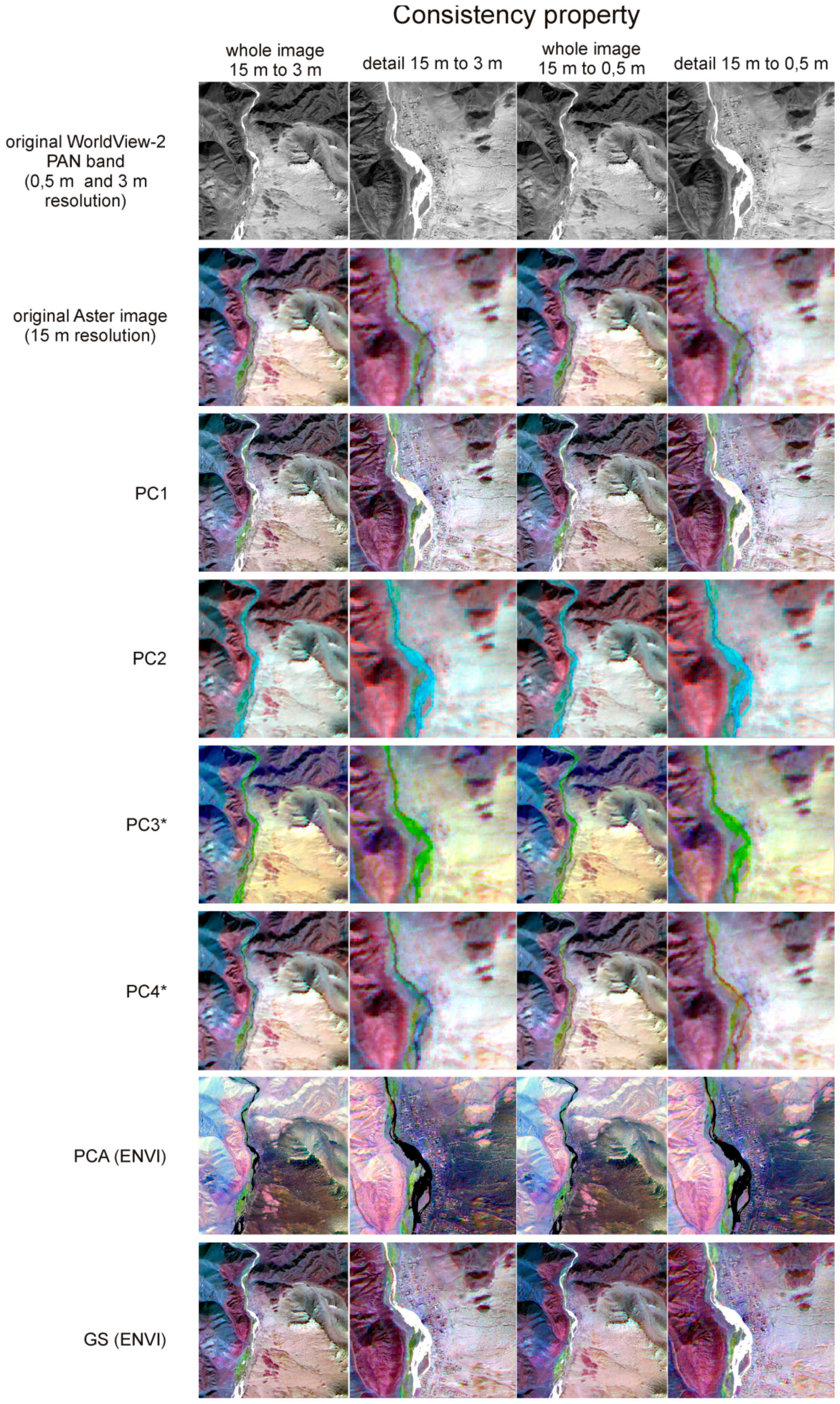
Consistency property: the sharpened image, once spatially degraded to the resolution of the original MUL image, should be as identical as possible to the original MUL image.

Synthesis property: combines the second and third property from Wald’s protocol, the first states that each band from the fused image should be as identical as possible to the respective band of the image that would be acquired by the sensor of same spatial resolution as the PAN image. The third property applies a similar requirement as the second property, but on a set of multispectral bands.

Validation for this study consisted of the following approaches: (i) visual inspection; (ii) consistency and synthesis property assessment; and (iii) spectral property assessment.

3.4.1. Consistency Property

The consistency property can be performed easily by degrading the fused image on to a spatial resolution of the original MUL image so the original MUL image can be used as the reference image in the validation process. The relative global dimensionless synthesis error (ERGAS) [34] is among the most popular validation metrics, however other widely used metrics are [10,11,30]: the spectral angle mapper (SAM), spectral information divergence (SID), root mean square error (RMSE), the band-to-band correlation coefficient (CC) or the universal image quality index (UIQI). The quantitative metrics requiring a reference image that were used in this study are summarized in

Table 2. The quality assessment metrics used in the study that require a reference image. (ERGAS: relative global dimensionless synthesis error; SAM: spectral angle mapper; UIQI: universal image quality index).

	Name	Formula	References
1	ERGAS	$ERGAS=100\frac{h}{l}\sqrt{\frac{1}{N}{\displaystyle {\displaystyle \sum }_{N=1}^N}{\left(\frac{RMSE\left(n\right)}{\mu \left(n\right)}\right)}^2}$	[34]
2	UIQI	$Q_j=\frac{{\sigma }_{xy}}{{\sigma }_x{\sigma }_y}\frac{2\widehat{x}\widehat{y}}{{\left(\widehat{x}\right)}^2+{\left(\widehat{y}\right)}^2}\frac{2{\sigma }_x{\sigma }_y}{{\sigma }_x^2+{\sigma }_y^2}$ $Q=\frac{1}{M}{\displaystyle {\displaystyle \sum }_{j=1}^M}{Q}_j$	[38]

.

3.4.2. Synthesis Property

The synthesis property is, in most cases, very difficult to validate [30]. As stated in [11], the general approach to deal with the synthesis property is to degrade the PAN band to the resolution of the original MUL image and to degrade the original MUL image in a way to keep the ratio of spatial resolutions. By doing this, the PAN sensor of the MUL resolution is simulated, so the synthesis property can be validated. The resulting fused image then has the same spatial resolution as the original MUL image and this image can then be used as a reference image in the validation process. As was stated in [30], fulfillment of the synthesis property is much harder than the consistency property, because the spatial degradation causes a loss of information from both MUL and PAN. In this study, the synthesis property was tested by creating synthetic images from the original ASTER/WorldView-2/Landsat 8 MUL and PAN images (

Table 3. Overview of input datasets for testing the synthesis property. Synthetic images were created in order to test the synthesis property of the fused image. Synthetic images were created to preserve the ratio between the original MUL and PAN images, when the PAN was synthetically degraded to the original resolution of the original MUL.

Sharpening Case	Input Datasest	Original	Synthetic	Sharpened Result
1	Landsat 8 MUL	30 m	60 m	30 m
	Landsat 8 PAN	15 m	30 m
2	ASTER	15 m	450 m	15 m
	WorldView-2	0.5 m	15 m
3	ASTER	15 m	75 m	15 m
	WorldView-2	3 m	15 m

).

The second broadly accepted approach to deal with the lack of reference image, which is crucial especially in the case of the synthesis property requirement, is to use one of the quality indexes which do not require a reference image [10,11,30]. The most used index for this purpose is the quality index without reference (QNR), introduced in [19]. The advantage of the QNR is that it works at the level of a PAN image and thus there is no need to degrade the fused image. The index combines spectral and spatial distortion indexes by calculating the Universal Image Quality Index [38] at the inter-band level. Values of QNR are between 0 and 1; however a value equal to 1 is only achieved if the two compared images are identical. The formula (

Table 4. Definition of the quality without reference index (QNR). Parameters p, q, α, and β were set to 1, as is recommended in [19].

	Name	Formula	References
1	QNR	$QNR={\left(1-D_{\lambda }\right)}^{\alpha }{\left(1-D_S\right)}^{\beta }$	[27]
	Spectral distortion	$D_{\lambda }=\sqrt[p]{\frac{1}{N\left(N-1\right)}{\displaystyle {\displaystyle \sum }_{i=1}^N{\displaystyle \sum }_{j=1,j\ne i}^N}{|Q\left(M{S}_i,M{S}_j\right)-Q\left({\widehat{\widehat{M}S}}_i,{\widehat{\widehat{M}S}}_j\right)|}^p}$
	Spatial distortion	$D_S=\sqrt[q]{\frac{1}{N}{\displaystyle {\displaystyle \sum }_{i=1}^N}{|Q\left({\widehat{\widehat{M}S}}_i,P\right)-Q\left(M{S}_i,P_{LP}\right)|}^q}$

) uses the multiplicative parameters p, q, α, and β, which are used for emphasizing either spectral (p and α) or spatial distortion (q and β), and are in default set to 1 [27].

3.4.3. Spectral Property Assessment

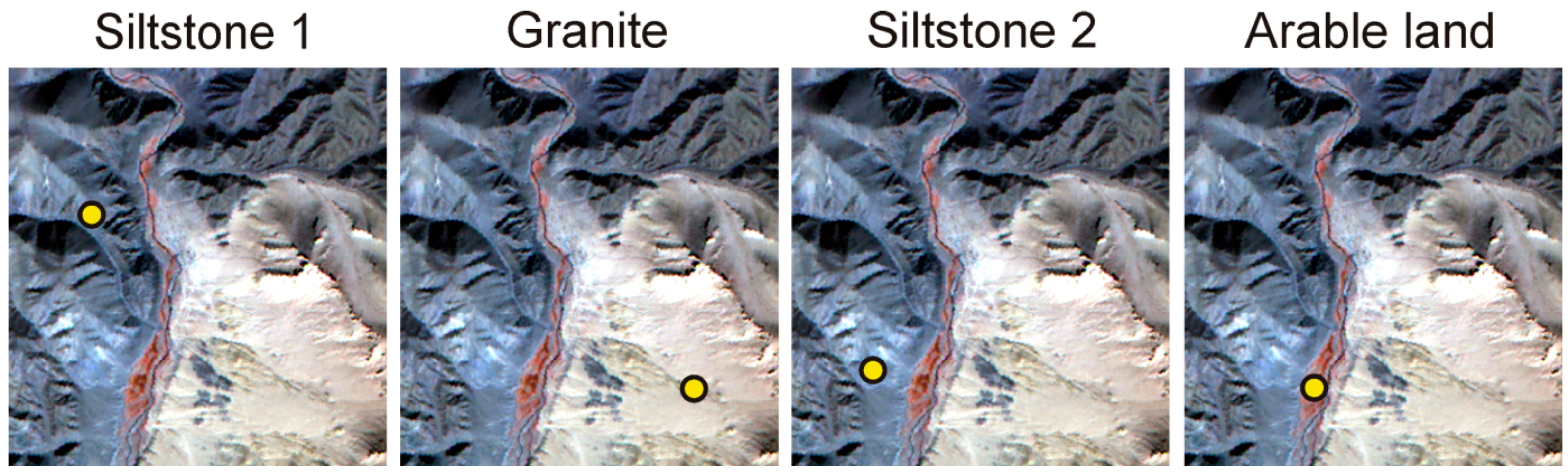
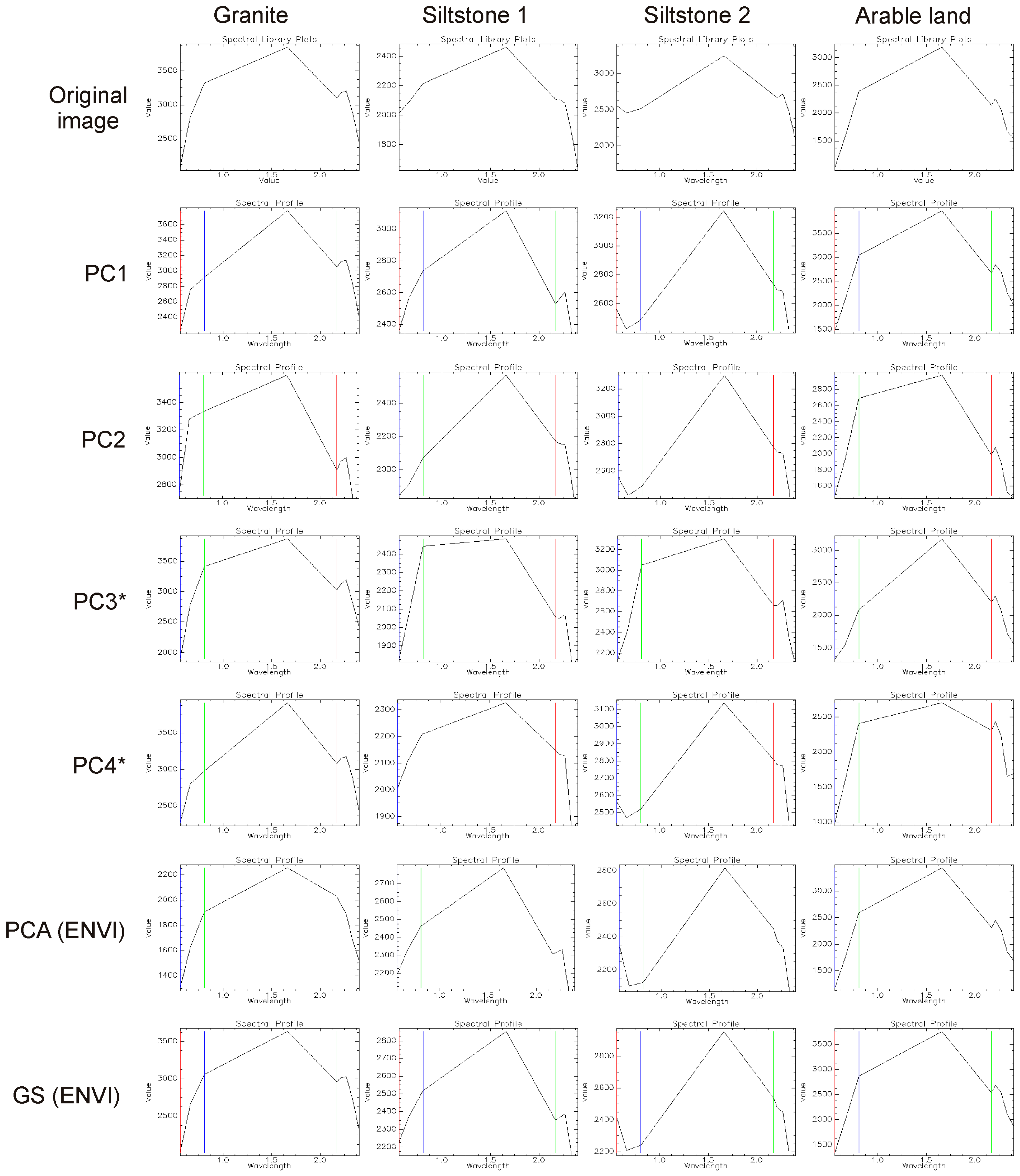
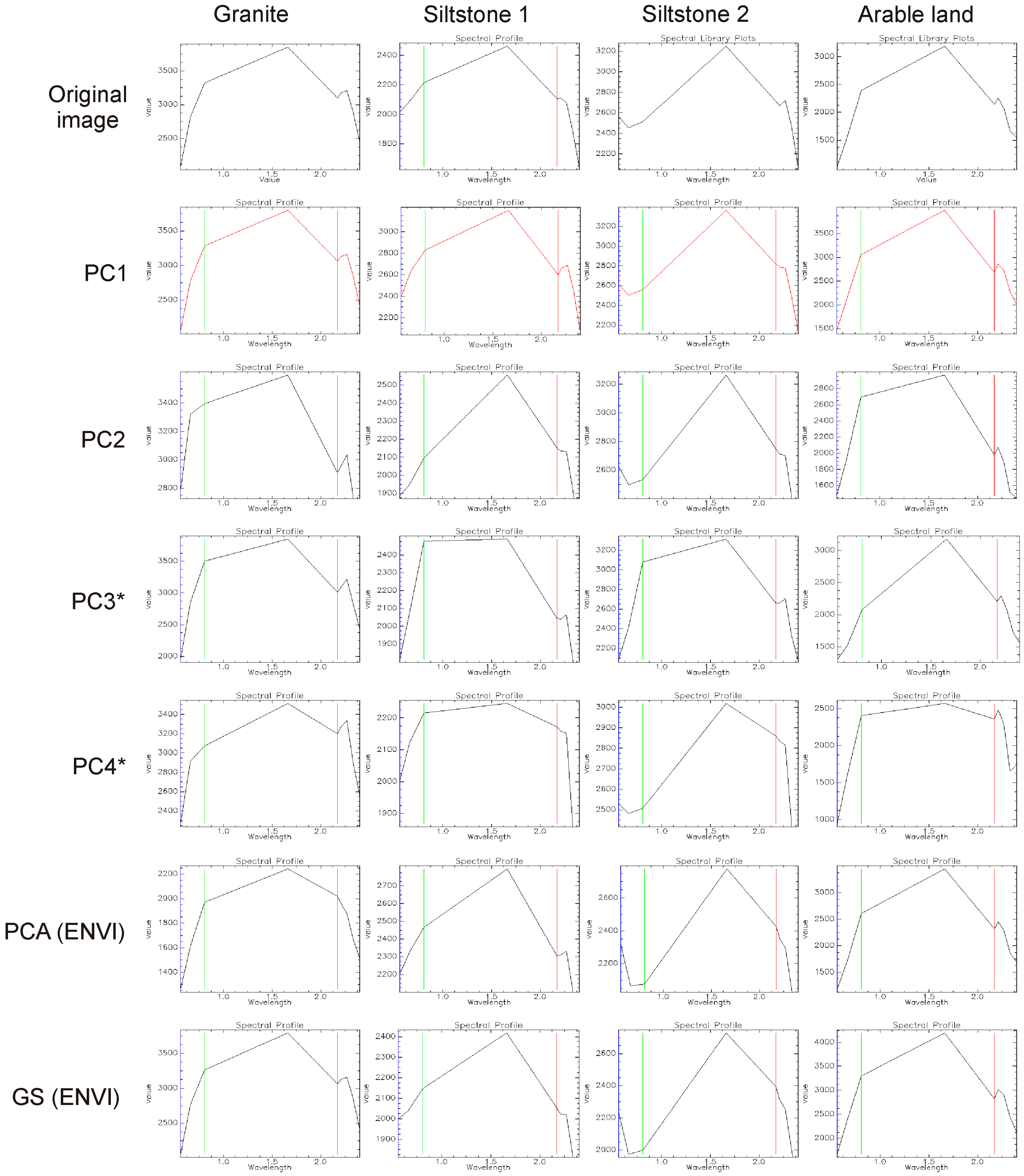
Four different surface types (Figure 5) that were found to be stable for those datasets with different date of acquisitions (ASTER and WV2 data acquisitions) were selected to assess the spectral quality. These surfaces showed differences in albedo within the ASTER and Landsat 8 scenes (granite, arable land, siltstone 1, siltstone 2: listed from the brightest to the darkest surfaces) as well as different absorption features (siltstone 2 shows well-pronounced absorption in the VNIR while weathered granite shows absorption in the SWIR due to the presence of clay minerals).

The original pixel reflectance spectra (ASTER, Landsat 8) and the corresponding spectra of the fused images were compared using the spectral angle (SAM, [39]) and the spectral feature fitting (SFF, [40]) metrics. To ensure that the reflectance of both reference Landsat 8 (30-m pixel)/ASTER (15-m pixel) and the fused products (15-m pixel /0.5- and 3-m pixels, respectively) represents comparable surfaces in terms of spatial extents, the SAM and SFF (both available in ENVI/Spectral analyst) were calculated between the reference image’s pixels and the corresponding spatial matrices of the pixels of all the fused products (2 × 2 pixels in the case of Landsat-8 fused images and 30 × 30 and 5 × 5 pixels in the case of ASTER fused products).

4. Results and Discussion

All of the derived sharpened products (4 sharpened images using PC1–PC4 for a substitution, ENVI GS and ENVI PCA sharpened images) computed for the Landsat 8 datasets and ASTER (0.5- and 3-m resolution) were validated for both the consistency and synthesis property using the ERGAS, UIQI and QNR indexes. Moreover, the spectra of the four different surfaces were evaluated using a visual inspection as well as two quantitative spectral metrics—SAM and SFF. The final observations are then formulated based on a complex assessment—visual, statistical and spectral.

4.1. Visual Inspection

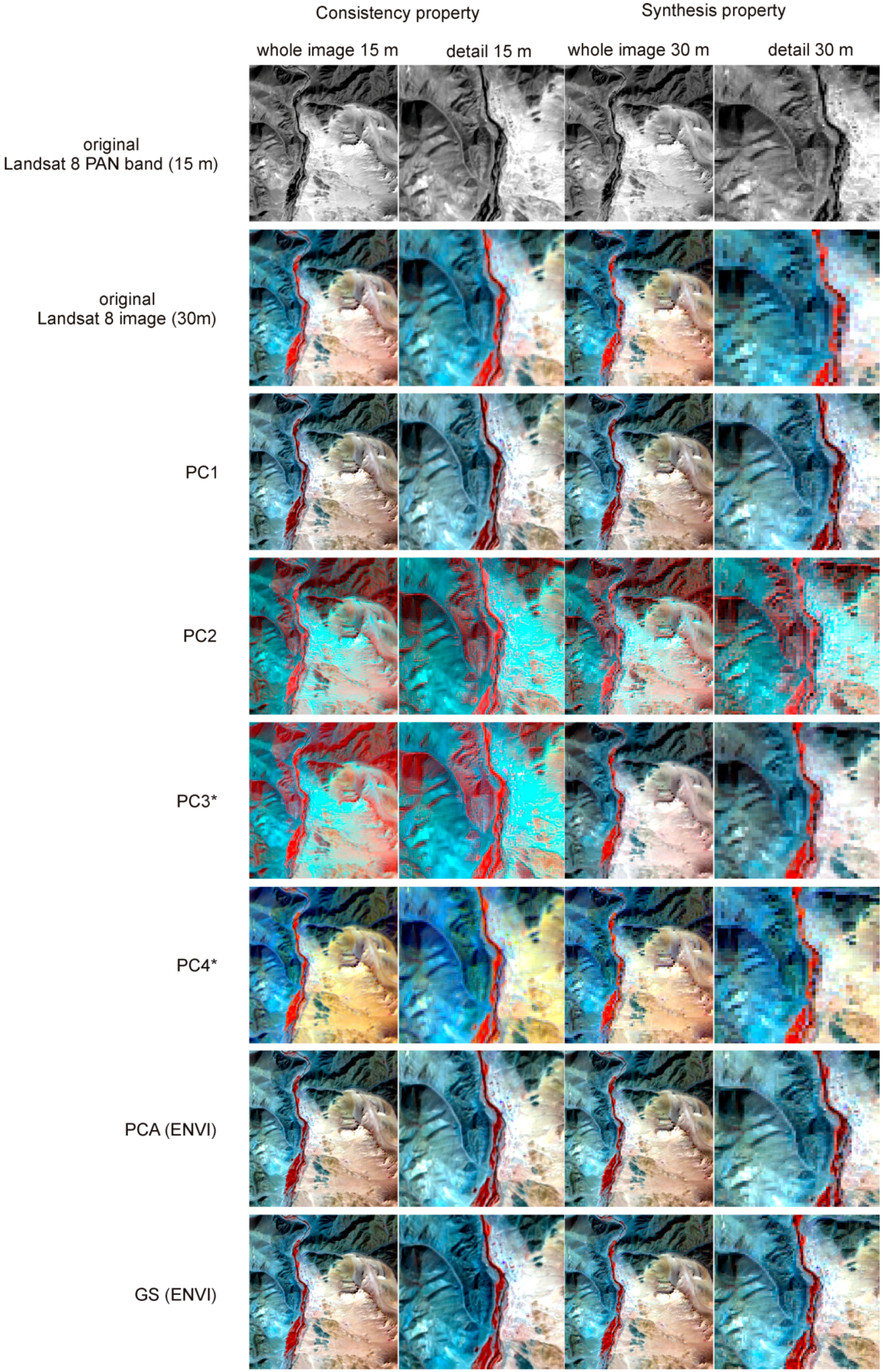
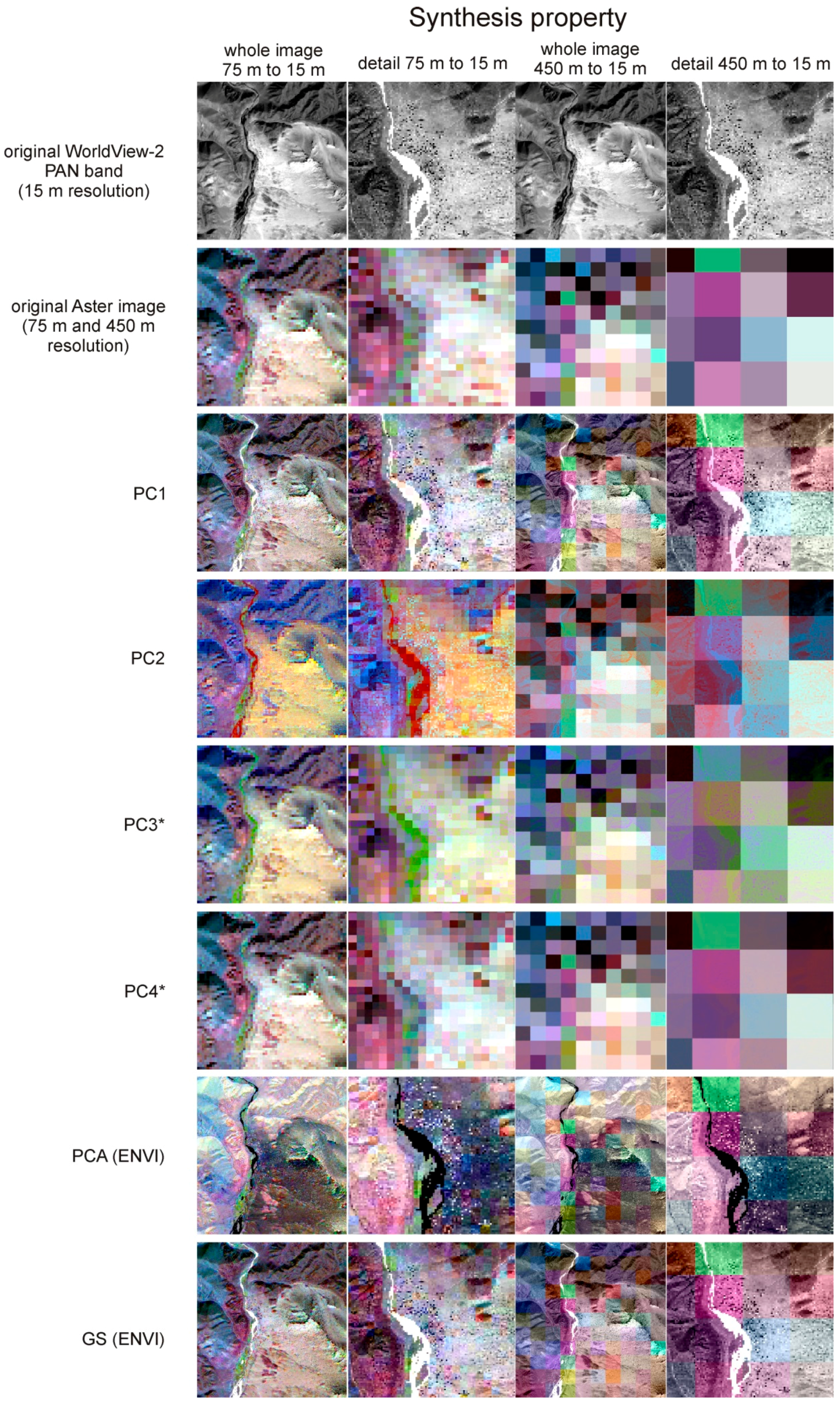
The visual analysis allows assessment of general image quality. For Landsat 8 (Figure 6), the visually comparable results were achieved using the newly proposed PCA approach using the PC1 in a substitution and both ENVI built-in methods (ENVI GS and ENVI PCA). However, when sharpening the datasets acquired by two different sensors and at different dates (ASTER MUL and WV2 PAN), the ENVI built-in PCA method resulted in a product exhibiting an inverse albedo (e.g., bright surfaces are dark and vice versa, Figure 7 and Figure 8). However, this problem did not occur, when either the PC1 or PC2 were used for substitutions when using the newly developed processing chain. These results are visually comparable to the ENVI GS sharpening method.

As expected, when using PC3 and PC4—the PCs that do not contain high enough data variability—the effect of spatial enhancement was lost in the fused product. The results obtained demonstrate that only PC1 and PC2 are relevant for preserving high spatial content.

4.2. Statistical Assessment

A quantitative quality assessment was performed on two levels as is implied from Wald’s protocol, which includes testing the consistency and synthesis property of the fused image. As was stated above, the consistency property of the fused image means, if generalized, that the resulting image is resampled back to the spatial resolution of the original image and compared with the original MUL image which serves as the reference image in this case. The synthesis property of the fused image means, if generalized, that the fusion is carried out on two spatially degraded images, where the original PAN band is spatially resampled to the resolution of the original MUL image and the original MUL image is then spatially degraded to retain the same ratio between the spatial resolutions of the original MUL and PAN.

The consistency property involved one Landsat 8 result (15-m spatial resolution) resampled back to the 30-m resolution and two ASTER results (0.5- and 3-m spatial resolution), resampled back to the resolution of 15-m. The synthesis property involved one Landsat 8 result at the 30-m resolution and two ASTER fusion results, both at the 15-m resolution (Table 3). ERGAS [34] and UIQI [38] are the quality indexes used in this study. In addition, QNR [27], as the commonly used index that does not need any reference image, was used as the alternative to the synthesis property validation. For ERGAS, the best possible result is zero, which in fact indicates two identical images. Common values presented in the literature for sharpening algorithms vary between 1 and 3 [28,33,41]. Values of the UIQI range from +1 to −1, while 1 is considered to be the best value. Values of the QNR vary between 0 and 1, the closer to 1 the result is, the more similar to the original image the fused image is.

Table 5. ERGAS values for the Landsat 8 dataset. * Sharpened images for the synthesis property were created from synthetic images where PAN was degraded to the resolution of the original MUL (30-m) and the MUL was thereafter degraded to 60-m in order to keep the same spatial resolution ratio. For ERGAS, the best possible result is zero, which indicates two identical images. It was expected that the first two PCs have the potential to give good results when employing the PCA sharpening process, however PC3* and PC4* were used to compare the result and explain it in a wider context.

ERGAS	Consistency	Synthesis
Spatial resolution	15-m	30-m (60-m)
PC1	4.06198	3.07587
PC2	5.17874	6.0137
PC3*	3.31786	2.91212
PC4*	2.98782	2.66469
ENVI GS	2.07082	2.24123
ENVI PCA	2.59029	2.68534

and

Table 6. ERGAS values for ASTER dataset.* Sharpened images for synthesis property were created from synthetic images where the PAN was degraded to the resolution of the original MUL (15-m) and the MUL was thereafter degraded to 450-m and 75-m respectively in order to keep the same spatial resolution ratio. For ERGAS, the best possible result is zero, which indicates two identical images. It was expected that the first two PCs have the potential to give good results when employing the PCA sharpening process, however PC3* and PC4* were used to compare the result and explain it in a wider context.

ERGAS	Consistency		Synthesis
Spatial resolution	0.5-m	3-m	15-m (450-m)	15-m (75-m)
PC1	0.584261	3.50611	0.634291	3.63702
PC2	0.652684	3.91483	0.814518	3.95748
PC3*	0.319882	1.9179	0.807194	3.17371
PC4*	0.193797	1.12199	0.787063	2.61341
ENVI GS	0.67202	4.22943	0.775266	4.32383
ENVI PCA	1.68028	10.1658	1.78183	10.2482

present ERGAS values obtained for Landsat 8 and ASTER results respectively. ERGAS measures the global error, which is mostly driven by the spectral deviation between two compared images. Comparing 0.5- and 3-m spatial resolution ASTER products, lower ERGAS values, and thus better results, are achieved for the 0.5-m spatial resolution (for both consistency and synthesis). For both ASTER products (0.5- and 3-m spatial resolution), the modified PCA approach brought significantly better results than ENVI PCA (Table 6). The new approach using PC1 and PC2 methods exhibit better ERGAS values in both the consistency and synthesis properties than the ENVI PCA method (PC1: ERGAS 0.58: (0.5-m) and 3.5 (3.5-m) in comparison with ERGAS: 1.68 (0.5-m) and 10.17 (3.0-m), respectively, for ENVI PCA). The newly proposed method was able to get similar or even better ERGAS values (ERGAS: 0.58 (0.5-m resolution) and 3.51 (3.0-m resolution) than for the ENVI GS (ERGAS: 0.67 (0.5 m resolution) and 4.23 (3.0-m resolution)) in the consistency property and 0.63/3.64 versus 0.78/4.32 in the synthesis property. The best ERGAS values (ERGAS: 0.32 and ERGAS: 0.20 respectively) are recorded when using PC3 and PC4 in the sharpening process. The resulting sharpened images in both cases have a high degree of suppression of the spatial content from the WV2 PAN band and, as mentioned before, these are not useful sharpening products (Table 6).

In the case of the Landsat 8 dataset, the proposed modified PCA approach was not able to surpass the ERGAS values of ENVI PCA and GS. The synthesis property (Table 5) gave a comparable ERGAS result to the ENVI methods (PC1: 3.08 versus ENVI GS: 2.24 and ENVI PCA: 2.69), on the other hand, evaluating the consistency property (Table 5) the results were significantly better while using the ENVI method.

Comparing the results with the published literature, values are within the range that can be considered as acceptable/good results. For WV2 datasets (using in-house PAN band) [6,10,11,30], values range from 1.7 using GS [30] to 5.91 using a modified PCA [10]. For Landsat-7 datasets (using in-house PAN band), values range from 7.27 to 8.75 [10].

Table 7. Interband UIQI for Landsat 8 dataset. Values of the UIQI range from +1 to −1, while 1 is considered as the best value. PC3* and PC4* were used to compare the result and explain it in a wider context.

Consistency 30-m
	PC1	PC2	PC3*	PC4*	PCA ENVI	GS ENVI
b1	0.884885	0.807992	0.772405	0.660137	0.952822	0.957801
b2	0.873974	0.82019	0.791765	0.758381	0.947333	0.953344
b3	0.823249	0.905313	0.861151	1	0.920236	0.932006
b4	0.765444	0.939935	0.93497	0.912478	0.887502	0.906047
b5	0.687548	0.151905	0.987592	0.986964	0.832086	0.866993
b6	0.692889	0.999814	0.967739	0.988492	0.836537	0.868202
b7	0.735425	0.872152	0.958945	0.967745	0.868963	0.894791
mean	0.780487	0.785328	0.896367	0.896314	0.892213	0.911312
Synthesis 30-m
	PC1	PC2	PC3*	PC4*	PCA ENVI	GS ENVI
b1	0.888327	0.808471	0.806283	0.472138	0.895438	0.907212
b2	0.89221	0.815688	0.816434	0.527942	0.902146	0.914358
b3	0.890696	0.836943	0.835211	0.74691	0.912847	0.926828
b4	0.856817	0.829604	0.826913	0.806897	0.889912	0.905602
b5	0.763934	−0.0088408	0.788224	0.722062	0.805121	0.825498
b6	0.781406	0.754746	0.663179	0.767714	0.821331	0.839523
b7	0.817045	0.810545	0.663683	0.705063	0.854096	0.870666
mean	0.841492	0.692452	0.771417	0.678389	0.8687	0.884243

and

Table 8. Interband UIQI for Aster dataset. Values of the UIQI range from +1 to −1, while 1 is considered as the best value. PC3* and PC4* were used to compare the result and explain it in a wider context.

Consistency (0.5-m)
	PC1	PC2	PC3*	PC4*	PCA ENVI	GS ENVI
b1	0.61	0.41	0.53	0.99	0.23	0.53
b2	0.51	0.48	1	0.99	−0.01	0.4
b3	0.45	0.62	0.65	1	−0.07	0.4
b4	0.29	0.6	1	0.53	−0.16	0.32
b5	0.29	0.57	0.91	0.87	−0.16	0.32
b6	0.29	0.6	0.97	0.88	−0.13	0.33
b7	0.27	0.62	1	0.9	−0.19	0.29
b8	0.28	0.65	0.93	1	−0.17	0.31
b9	0.3	0.76	0.99	0.87	−0.18	0.32
mean	0.37	0.59	0.89	0.89	−0.09	0.36
Consistency (3-m)
	PC1	PC2	PC3*	PC4*	PCA ENVI	GS ENVI
b1	0.42	0.33	0.3	0.61	0.18	0.64
b2	0.39	0.4	0.67	0.67	−0.04	0.55
b3	0.36	0.51	0.54	0.7	−0.08	0.5
b4	0.25	0.48	0.79	0.55	−0.16	0.32
b5	0.25	0.44	0.7	0.65	−0.16	0.33
b6	0.25	0.46	0.75	0.67	−0.13	0.33
b7	0.23	0.47	0.76	0.67	−0.19	0.3
b8	0.25	0.51	0.72	0.78	−0.17	0.31
b9	0.26	0.58	0.76	0.64	−0.18	0.34
mean	0.3	0.46	0.67	0.66	−0.1	0.4
Synthesis (15-m from 75-m)
	PC1	PC2	PC3*	PC4*	PCA ENVI	GS ENVI
b1	0.336513	−0.20047	−0.00759	0.25486	−0.18246	0.343825
b2	0.339347	−0.16378	0.213038	0.200989	−0.24714	0.358754
b3	0.320084	−0.05674	0.326748	0.228391	−0.2447	0.347763
b4	0.223907	0.360738	0.361293	0.393881	−0.21657	0.240373
b5	0.230236	0.333263	0.275764	0.222328	−0.19912	0.263554
b6	0.219133	0.330798	0.305667	0.239916	−0.18132	0.244568
b7	0.22319	0.344311	0.324502	0.219498	−0.21534	0.250268
b8	0.219179	0.37002	0.299869	0.349303	−0.22336	0.231999
b9	0.239196	0.349138	0.30034	0.18724	−0.22421	0.268403
mean	0.261199	0.185253	0.266626	0.255157	−0.21491	0.283278
Synthesis (15-m from 450-m)
	PC1	PC2	PC3*	PC4*	PCA ENVI	GS ENVI
b1	0.333633	0.267856	−0.18723	−0.04755	−0.29579	0.324758
b2	0.35204	0.265348	−0.03899	0.005559	−0.31167	0.351947
b3	0.331123	0.234576	0.188579	0.010597	−0.29739	0.335863
b4	0.23871	−0.16392	0.040891	−0.11551	−0.22313	0.246873
b5	0.236414	−0.15282	−0.03703	0.064194	−0.22467	0.247466
b6	0.22244	−0.11537	−0.02501	0.110881	−0.20705	0.231169
b7	0.241983	−0.13272	−0.00578	0.075803	−0.22408	0.253628
b8	0.23906	−0.16402	−0.03532	−0.02236	−0.22178	0.248802
b9	0.254419	−0.09992	−0.0448	0.076378	−0.24088	0.265469
mean	0.272201	−0.00678	−0.01608	0.017554	−0.2496	0.278442

present UIQI values for the Landsat 8 and ASTER datasets, respectively. Although usually used in a modification for multiband data, using UIQI for a single band to band comparison, the overall global accuracy at the band level is examined. This can show which band is well preserved and which is rather altered during the sharpening process.

The Landsat 8 dataset (Table 7) proved overall stability in high UIQI values throughout the bands and showed that this method although with lower values than ENVI methods, brings satisfactory results that are comparable with the results in [10], where the best value achieved was 0.9145 for the consistency property of Landsat-7 [10]. In the case of the ASTER dataset (Table 8), the overall scores of the UIQI proved that the proposed modified PCA approach has comparable results with the ENVI GS method when fusing ASTER and WV2 data. The results also show that using PC2 in substitution helps to preserve SWIR bands better than if the first PC is used.

Table 9. QNR for the Landsat 8 dataset. Values of the QNR vary between 0 and 1, the closer to 1 the result is, the more similar to the original image the fused image is. It was expected that the first two PCs have the potential to give good results when employing the PCA sharpening process, however PC3* and PC4* were used to compare the result and explain it in a wider context.

	Consistency	Synthesis
Spatial resolution	15-m	30-m (15-m)
PC1	0.872869	0.927271
PC2	0.533903	0.626443
PC3*	0.778605	0.792354
PC4*	0.613371	0.647593
GS ENVI	0.851012	0.954483
PCA ENVI	0.849988	0.957101

and

Table 10. QNR for the ASTER dataset. Values of the QNR vary between 0 and 1, the closer to 1 the result is, the more similar to the original image the fused image is. It was expected that the first two PCs have the potential to give good results when employing the PCA sharpening process, however PC3* and PC4* were used to compare the result and explain it in a wider context.

	Consistency		Synthesis
Spatial resolution	0.5-m	3-m	450-m (0.5-m)	75-m (3-m)
PC1	0.604003	0.689741	0.942421	0.899283
PC2	0.285938	0.407835	0.243406	0.486668
PC3*	0.411496	0.536061	0.331261	0.647254
PC4*	0.366688	0.525274	0.268338	0.648041
GS ENVI	0.566472	0.700017	0.936051	0.89261
PCA ENVI	0.462558	0.5766	0.62859	0.645949

present results of the QNR index for the Landsat 8 and ASTER datasets respectively. QNR is an index based on the UIQI, which serves as one of the most accepted indexes with no reference image needed [11]. The results for the Landsat 8 dataset are summed in Table 9 and for the ASTER dataset in Table 10. In general, the best values are achieved for the Landsat dataset, which is given by the fact that this dataset is more inherent. The poorer results obtained for the ASTER-WV2 sharpening scenario when compared to Landsat 8 sharpening scenario can be explained by the fact that images of different origin (sensor and data acquisition) were fused together, which is usually a more difficult task than sharpening data of the same origin, like Landsat-8. In all cases, with the exception of Landsat synthesis, the modified PCA approach using PC1 in the substitution achieved better values than the ENVI PCA (0.5 m ASTER—QNR: 0.6 and Landsat 8 datasets—QNR: 0.87). Furthermore, in most cases the PC1 substitute performed comparably or even better than the ENVI GS. In comparison with reference literature, where the values for WV2 ranged from 0.82 using PCA [30] to 0.97 [10] and for Landsat 7 being around 0.95 [10,37], these results show lower values, but are still within the acceptable range.

4.3. Spectral Property Assessment

The spectral performance of the sharpening algorithm is a crucial part of any sharpening method. To validate spectral quality, four types of surfaces showing differences in albedo were chosen (Figure 5): granite, siltstone 1, siltstone 2 and arable land.

Figure 9 and Figure 10 refer to the 0.5-m and 3.0-m sharpened products of ASTER. The problem of the albedo inversion for the ENVI PCA sharpening method is also demonstrated in this case, as the bright target, granite, has lower reflectance values than the dark target, the siltstones. Although the shape of the spectrum seems to be preserved at a satisfactory level (

Table 11. SAM and SFF scores achieved when comparing the Landsat 8 reference and the fused image spectrum. The higher the score the higher the match (0: no match, 1: identical spectrum). It was expected that the first two PCs have the potential to give good results when employing the PCA sharpening process, however PC3* and PC4* were used to compare the result and explain it in a wider context.

	Granite	Siltstone 1	Siltstone 2	Arable Land
SAM
PC1	0.956	0.989	0.921	0.809
PC2	0.919	0.989	0.963	0.973
PC3*	0.984	0.985	0.953	0.814
PC4*	0.959	0.961	0.972	0.665
ENVI GS	0.984	0.976	0.972	0.921
ENVI PCA	0.978	0.969	0.961	0.879
SFF
PC1	0.974	0.969	0.993	0.823
PC2	0.68	0.969	0.895	0.931
PC3*	0.978	0.992	0.97	0.81
PC4*	0.675	0.732	0.837	0.978
ENVI GS	0.982	0.968	0.996	0.857
ENVI PCA	0.978	0.961	0.995	0.775

,

Table 12. SAM scores achieved when comparing the ASTER reference and the fused image spectrum. The higher the score the higher the match (0: no match, 1: identical spectrum). It was expected that the first two PCs have the potential to give good results when employing the PCA sharpening process, however PC3* and PC4* were used to compare the result and explain it in a wider context.

SAM	Granite	Siltstone 1	Siltstone 2	Arable land
0.5-m
PC1	0.945	0.971	0.987	0.955
PC2	0.867	0.933	0.983	0.842
PC3*	0.968	0.936	0.888	0.909
PC4*	0.944	0.967	0.968	0.879
ENVI GS	0.985	0.982	0.974	0.965
ENVI PCA	0.944	0.984	0.966	0.982
3-m
PC1	0.999	0.967	0.986	0.956
PC2	0.863	0.948	0.984	0.839
PC3*	0.964	0.928	0.878	0.911
PC4*	0.927	0.948	0.943	0.845
ENVI GS	0.997	0.988	0.955	0.932
ENVI PCA	0.949	0.983	0.96	0.983

and

Table 13. SFF scores achieved when comparing the ASTER reference and the fused image spectrum. The higher the score the higher the match (0: no match, 1: identical spectrum). It was expected that the first two PCs have the potential to give good results when employing the PCA sharpening process, however PC3* and PC4* were used to compare the result and explain it in a wider context.

SFF	Granite	Siltstone 1	Siltstone 2	Arable land
0.5-m
PC1	0.998	0.983	0.897	0.869
PC2	0.993	0.977	0.905	0.941
PC3*	0.977	0.971	0.713	0.818
PC4*	0.999	0.943	0.863	0.853
ENVI GS	0.999	0.981	0.845	0.899
ENVI PCA	0.769	0.981	0.845	0.951
3-m
PC1	0.999	0.988	0.913	0.867
PC2	0.973	0.976	0.896	0.955
PC3*	0.971	0.969	0.701	0.837
PC4*	0.904	0.942	0.765	0.834
ENVI GS	1	0.968	0.84	0.833
ENVI PCA	0.769	0.979	0.841	0.927

), the albedo inversion was identified as the major problem for this method when fusing the dataset from a different origin (sensors and date of acquisition).

When assessing the spectral performance (Figure 9 and Figure 10 and Table 11, Table 12 and Table 13), the ENVI GS sharpening method performs as well as the modified PCA approaches when the PC1 and PC2 are used for the substitution. When using PC3 and PC4, the spectrum is not well preserved, mainly in the VIS part of the spectrum. However, as already explained, these two components are not suitable for the sharpening approaches.

Interestingly, the reflectance values are best preserved when PC2 is used for a substitution in the Landsat 8 dataset and also for the ASTER dataset (at both spatial resolutions 0.5- and 3.0-m, respectively). The fusion product using PC2 in a substitution brings even better results when the datasets of different sensor origin and, most importantly, of different acquisition time are fused, and when there are different illumination conditions in the image data. For sharpening process, data with the same or the closest acquisition time are optimal; however such data are not always available. In such cases, different light/shadow conditions can affect spectral properties when substituting the first PC. The presented approach was able to overcome such difficulties using the PC2 in a substitution.

The SAM score shows (Table 12 and Table 13) that a better spectral match is achieved for the 3.0-m resolution fused ASTER products, however if the SFF parameter is used as a measure of spectral performance, there are no significant differences for both the 0.5- and 3.0-m fused products, showing that the absorption features are preserved at a satisfactory level even for 0.5 m spatial resolution products. When confronting the spectra for the selected surfaces on ASTER results (Figure 10) together with the SAM and SFF computed scores, it seems that the SFF parameter might be more suitable for this type of assessment, as sometimes rather high SAM scores are computed but the spectrum differs from the reference one. For instance, the SAM score for the PC3 product (3.0-m resolution) in the case of siltstone 2 is 0.878; however, the spectrum does not perform well when compared to the original ASTER spectrum (reference spectrum). The SFF score is then the lowest of all giving a value of 0.701. The same can be observed in the case of granite in ENVI’s PCA, where the spectrum differs from the reference one, which is visible at the SFF (0.769) result rather than at the SAM (0.949). In comparison with recent studies [10,11,30,37], which worked with similar datasets, using same sensor PAN bands, either WorldView-2 (worst 0.985 [37] using PCA, best 0.998 [30] using PRACS method proposed by [42]) or the Landsat-7 (ranging from 0.986 to 0.989 [10]), SAM values [10,11,30,37] were slightly better than the presented values.

Figure 9 and Figure 10 also show that if PC1 is used, the VNIR part of the spectrum is preserved better than if PC2 is used for a substitution. However, the SWIR part of the spectrum and the SWIR absorptions are preserved best of all if PC2 is used in the sharpening process. The same results were also demonstrated using the UIQI for both the ASTER and Landsat 8 datasets (Table 7 and Table 8; note, that PC3 and PC4 are not considered).

4.4. Summary on Validation

Diverse approaches to validate the fusion results have been used in this study. When summarizing the results coming from the validation of the consistency and synthesis property using the ERGAS, UIQI and QNR indexes, it can be stated that ENVI-based methods perform the best on Landsat 8 data. This is the dataset which represents an easier image sharpening example, as the Landsat 8 PAN, which is acquired simultaneously with the Landsat 8 MUL bands, is used for the sharpening. In this case, both datasets (MUL and PAN) have the same illumination/shadowing conditions.

On the other hand, when employing sharpening on the datasets such as the ASTER MUL bands and WV2 PAN band, this newly suggested method performs better than the ENVI GS method. Moreover, the ENVI PCA method does not provide acceptable results due to the aforementioned problem with the albedo inversion. It was also demonstrated that it is beneficial to use PC2 in the substitution, as it can help to prevent the loss of the albedo information and a consequent albedo inversion issue; moreover, the spectrum in the SWIR2 was preserved better when compared to the scenario if the PC1 was used in the substitution. When using the new approach, the results show that the data can be successfully sharpened to the original spatial resolution of the WV2 PAN band (0.5 m), as even better validation results given by ERGAS, UIQI have been achieved for a 0.5-m sharpened product than for one with a 3-m pixel size. The SAM and SFF scores also indicate that the spectrum of the 0–5 m product shows high similarity with the original one.

It seems that ERGAS is not sensitive enough to assess spectral property in detail as very good results were shown for PC3 and PC4 substitution scenarios, however the spectra were not well-preserved, as demonstrated in Table 12 and Table 13 and Figure 9 and Figure 10. Therefore it is recommended to use SAM and SFF in addition to ERGAS, similarly as used by [43].

5. Conclusions

There is a wide variety of newly proposed sharpening algorithms across the literature, however, as they require programming in different languages, they are not easy to implement for a wide community of users. In this study, it was demonstrated that the performance of the PCA sharpening method available in the ENVI software is not satisfactory in the case of fusing data coming from different sensors. A new approach was introduced which offers easy implementation, a modified version of the principal component analysis (PCA) sharpening algorithm. The newly proposed processing chain, which is a modification of the widely used PCA method and employs a new histogram matching workflow, is recommended for a scenario where datasets from two different sensors are fused. The visual assessment as well as all the spectral quality indicators (SAM, and SFF) and global indexes (ERGAS, UIQI, and QNR) proved that the spectral performance of the proposed modified PCA sharpening approach when employing PC1 and PC2 performs better than the ENVI PCA method in the case where datasets of different origin are used for fusion. Moreover, comparable or even better results are achieved in comparison to the Gram–Schmidt sharpening method (ENVI GS), which is commonly used by a wide part of the remote sensing community.

It was demonstrated that using the second principal component (PC2) in the sharpening workflow instead of the first component (PC1) can, to some extent, give better spectral performance of the sharpened image, especially in the case of fusing data of different sensors and acquisition times. Substituting the second PC can in this case overcome the loss of albedo information, which is mostly included in the first PC.

Furthermore, when the PC1 was used, the VNIR part of the spectrum was preserved better, however, if the PC2 was used, the SWIR part was preserved better. This demonstrates that this approach, which can be easily implemented and managed by a wide variety of users, can give a kind of flexibility. The users can process and check the spectral performance depending on the desired minerals (e.g., choosing the first component (PC1) when targeting minerals rich in Fe³⁺ or choosing the second component (PC2) when targeting clay minerals and carbonates). They can use either of the PC1 or PC2 approaches; however they can also combine both.

As demonstrated, the new histogram matching workflow helped to improve the PCA performance reaching a comparable and in some cases even better performance than the Gram–Schmidt algorithm. However, there is a bigger potential in this direction, more modifications in the histogram matching workflow should be tested in order to further enhance the quality of the sharpening methods in future.

In general, this study brings a contribution to a very important topic. Fusion between high spatial-resolution image data and superspectral or even hyperspectral data is becoming extremely relevant (e.g., [43,44]) when the new-generation superspectral satellite—Sentinel 2—was launched in June 2015, and, moreover, when the new hyperspectral satellites will be operating in orbit in the near future (e.g., EnMAP from 2018).