Article

On the Use of Cross-Correlation between Volume Scattering and Helix Scattering from Polarimetric SAR Data for the Improvement of Ship Detection

Institute of Photogrammetry and Remote Sensing, Chinese Academy of Surveying & Mapping, Beijing 100830, China
*
Author to whom correspondence should be addressed.
Remote Sens. 2016, 8(1), 74; https://doi.org/10.3390/rs8010074
Submission received: 12 October 2015 / Revised: 31 December 2015 / Accepted: 14 January 2016 / Published: 20 January 2016

Abstract

:
Synthetic Aperture Radar (SAR) ship detection is an important maritime application. However, azimuth ambiguities caused by the finite sampling of the Doppler spectrum are often visible in SAR images and are always mistaken as ships by classic detection techniques, like the Constant False Alarm Rate (CFAR). It is known that radar targets and azimuth ambiguities have different characteristics in polarimetric SAR (PolSAR) data, i.e., first ambiguities usually have strong odd- or double-bounce scattering and the maximum amplitude of the first ambiguity in SHV is always considerably smaller than that of the corresponding target for zero or high velocity. On the basis of this characteristics, this paper finds that first ambiguities usually have low volume scattering power relative to ships and almost have no helix scattering by Yamaguchi decomposition. But some residual ambiguities still exit in the volume scattering power and have similar scattering intensity to small ships, and some parts of a ship also have zero helix scattering owing to some physical factors (e.g., ship structure, radar incidence angle, etc.). Thus, for high-precision ship detection, a new ship detection method based on cross-correlation between the volume and helix scattering mechanisms derived from Yamaguchi decomposition is proposed to avoid false alarms caused by azimuth ambiguities and enhance Target-to-Clutter Ratio (TCR) for improving the miss detection rate of small ships. By experiments, it is proved that our method can work effectively and has high detection accuracy.

Graphical Abstract

1. Introduction

Synthetic Aperture Radars (SARs) have an important application for ship detection in the field of maritime security. Ships on the sea surface usually have stronger backscattering intensity than sea clutter and are displayed as bright spots in SAR images. Meanwhile, azimuth ambiguities caused by the discrete sampling of the Doppler frequency signal also have strong backscattering intensity relative to sea clutter and are often visible in SAR images [1,2,3]. Thus, the ambiguities are always mistaken as ships by some conventional ship detection methods, such as the Constant False Alarm Rate (CFAR) [4].
Several methods to resolve azimuth ambiguities have been investigated with single polarization SAR images. Moreira utilized an ideal filter concept to accommodate the undefined phase of the ambiguities and also the fading of the azimuth signal [5]. Monti Guarnieri also proposed an algorithm to suppress strong azimuth ambiguities in Single-Look Complex (SLC) SAR images. The algorithm exploits a band-pass filter to select that portion of the azimuth spectrum that is less influenced by aliasing [6]. Di Martino et al. proposed the AM and SF (asymmetric mapping and selective filtering) method based on the theory of selective filtering to suppress ambiguities [7].
For polarimetric SAR (PolSAR) data, Liu et al. found the different property between radar-observed targets and azimuth ambiguities. That is, the phase difference between HV and VH images is zero for reciprocal scatterers, whereas it is π for ambiguities and the ship detection operator |HV−VH| based on this property was proposed to distinguish ships from azimuth ambiguities [8,9,10]. Similarly, Velotto et al. also utilized the property by combining the cross-polarized channels of PolSAR data for removal of azimuth ambiguities [11,12]. For both the methods, HV and VH images have to be known firstly, which limits their extensive application. As we known, speckle in SAR images is a scattering phenomenon. Speckle filtering or multi-look processing is a procedure commonly adopted to reduce the speckle noise effect for SAR image interpretation. For PolSAR, the 1-look data can be represented by a scattering matrix S2. To form multi-look data, we can not average the scattering matrix S2, because the average of complex values will not reduce the speckle noise effect [13]. The proper way is to convert the scattering matrix S2 into a covariance C3 or coherency T3 matrix, and then a sample average is taken for speckle filtering. In other words, if we only have the coherence matrix (T3) or covariance matrix (C3) of PolSAR data but have no Sinclair scattering matrix (S2) in hand, HV and VH images can not be obtained. Therefore, neither of the two methods are suitable for distinguishing ships from azimuth ambiguities under these conditions. Additionally, Wang et al. analyzed the polarimetric characteristics of ships and azimuth ambiguities by Cloude-Pottier decomposition and found that the ambiguities in the third eigenvalue have lower intensity than ships and then the third eigenvalue was utilized to differentiate ships from azimuth ambiguities [2]. In general, this method can work effectively, but when residual azimuth ambiguities still appear in the third eigenvalues and have close Target-to-Clutter Ratio (TCR) to small ships, the ambiguities will also be mistaken as ships or some small ships will be missed by thresholding.
The small ship defined here usually has low TCR, owing to its physical factors (e.g., ship size, ship structure, and SAR imaging resolution, etc.). In order to detect small ships from sea clutter background, some classic detection methods utilize the coherence image derived from cross-correlation between two sub-look images of single polarization SAR image to increase TCR, such as two-looks internal Hermitian product (2L-IHP) [14], multi-look SAR images cross-correlation (MLCC) [15]. There exists a common characteristic that ships colocated in both sub-look images have strong correlation relative to the continuously changing sea clutter. It has been proved that those methods can enhance TCR, thereby benefiting small ship detection. However, these kind of detectors work with a reduced spatial resolution, compared with a single-look image detector. Therefore, from one hand they present a better TCR, but from the other hand they have a lower spatial resolution depending on the number of looks, and these detectors are suitable to a single polarization SAR image.
Thus, in order to extend ship detection to multi-look PolSAR data for avoiding false alarms generated from azimuth ambiguities and improving the missed detection rate of small ships, a new ship detection method is developed based on cross-correlation between volume and helix scattering mechanisms derived from Yamaguchi four-component decomposition in this study. Firstly, this paper finds that azimuth ambiguities have low volume scattering intensity relative to ships and almost have no helix scattering by expriments. Then, considering sometimes ambiguities still have similar volume scattering to small ships and some parts of a ship also have no helix scattering, the proposed method utilizes the two-dimensional convolution function (2D-CF) to get the coherence image of the volume and helix scattering mechanisms for further suppressing azimuth ambiguities and increasing TCR.

2. Azimuth Ambiguities Description

Azimuth ambiguities arise from the finite sampling of the Doppler frequency signal, which is weighted by the two-way azimuth antenna pattern. Doppler frequencies which are higher than the Pulse Repetition Frequency (PRF) are folded into the central part of the azimuth spectrum so that aliased signals will be produced. The ambiguities in SAR image displace spatially in azimuth (ΔxAZ) and range (ΔxRA) as follows [1]:
{ Δ x AZ n f p v / f DR Δ x RA n λ f p / f DR ( f DC + n f p / 2 )
where n is the number of ambiguities (n = ±1, 2, ... ), fp is the PRF, v is the velocity of a sensor platform and λ is the radar wavelength. fDR and fDC are the Doppler rate of the azimuth reference function and the Doppler centroid frequency, respectively.
fDR is calculated:
f DR = 2 v 2 cos 2 θ λ R 0
where θ is radar inclination angle, and R0 is the nearest distance between radar and observed target.
As shown in Equation (1), the displacement of azimuth ambiguities becomes larger with the increase of the wavelength if other parameters remain unchanged. Thus, the ambiguities are much closer to radar observed targets or within the area of interest in SAR images for a radar system of short wavelength. In other words, the ambiguities are less severe in SAR images of a long wavelength than of a short wavelength [2]. Therefore, several ghost ships generated from azimuth ambiguities will appear in C-band SAR images, whereas almost no ambiguities can be found in L-band SAR images correspondingly.
In 1993, Freeman analyzed the effects of noise on PolSAR data, and pointed out that ambiguities are unlike other forms of “noise” in that they can appear to be focused and look like “ghost” images [16], and in PolSAR data, only very bright odd- or double-bounce scatterers will produce azimuth ambiguities that look like fairly bright double- or odd-bounce scatterers, respectively [2,16]. Moreover, it has been proved in [10] that the amplitude of the first positive ambiguity in SHV increases as the target across-track velocity increases, but also begins to decrease beyond a certain velocity (e.g., 12 m/s as shown in [10]) and the maximum amplitude of the first ambiguity in SHV is always considerably smaller than that of the target image for zero velocity.

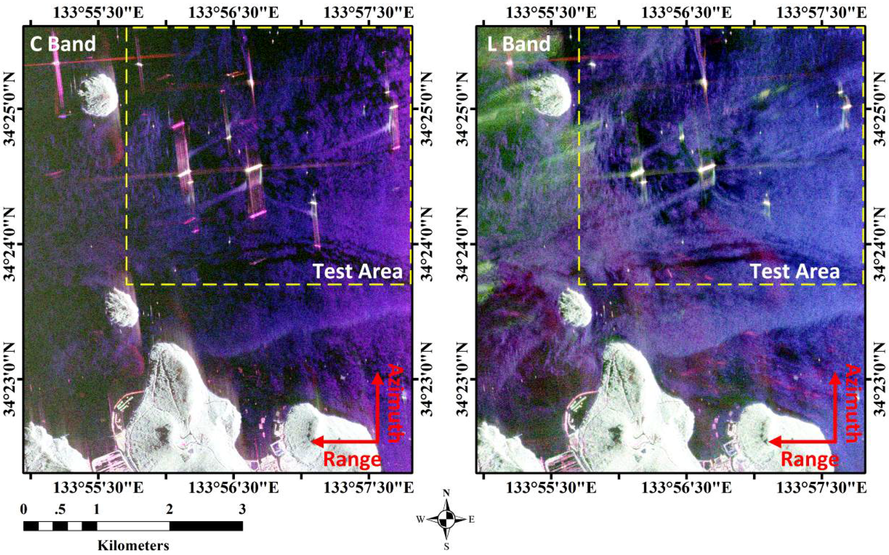
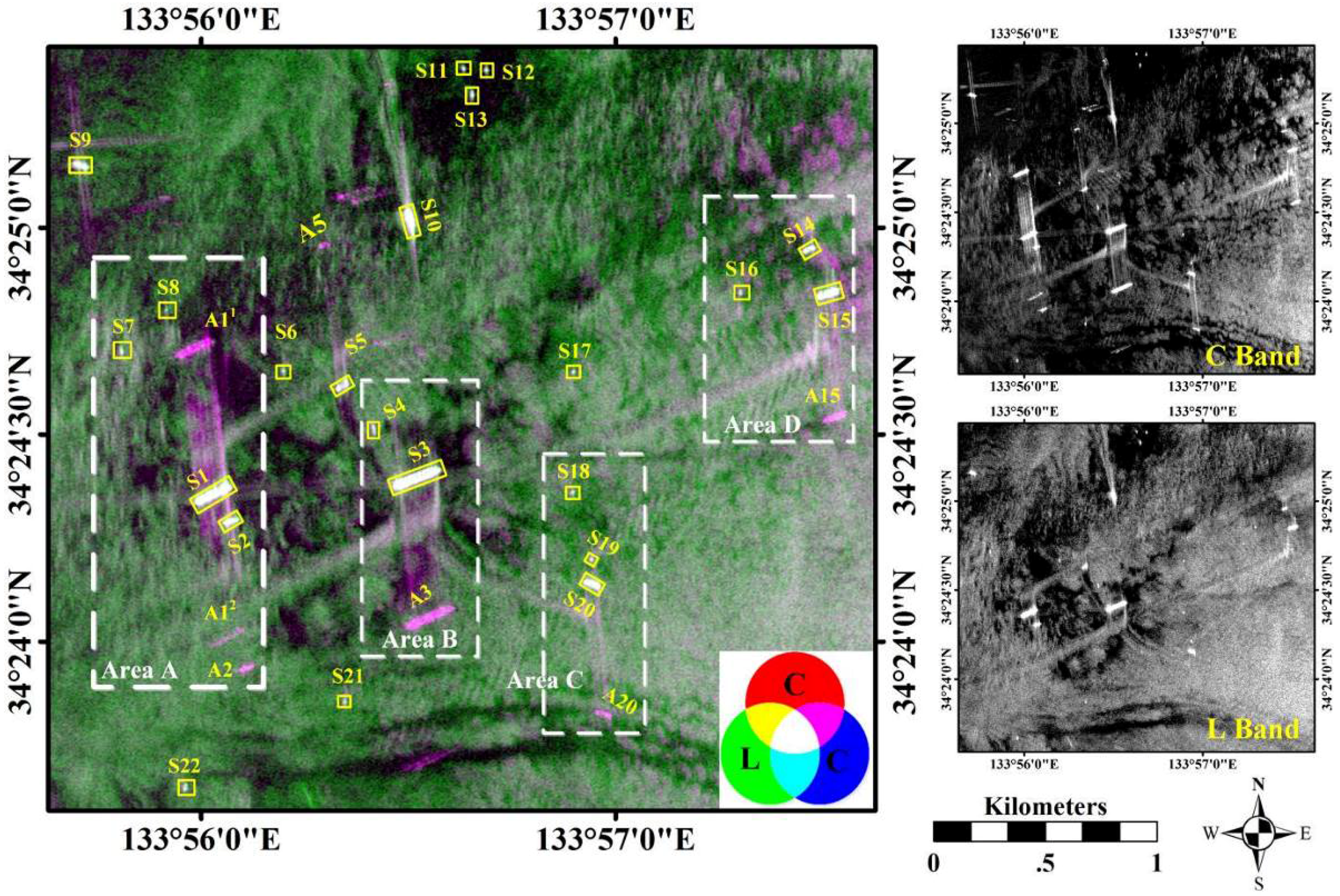
3. Experimental Data Description

In this study, a nine-look NASA/JPL AIRSAR polarimetric dataset acquired on 4 October 2000 was used for the experiments. The dataset consists of C-band and L-band PolSAR data and covers an area of the inland sea named Kojimawan, close to Tamano City, Japan. In order to avoid a lot of false alarms generated from land areas, we selected the test area outlined by the yellow dash line for the subsequent experiments (See Figure 1) and the main acquisition parameters of the dataset are listed in Table 1.
Due to the lack of the ground truth data about the ships on the sea surface, we previously have to interpret the ships visually with the pseudo-color RGB image, color coded by: red = C-band Span image (dB), green = L-band Span image (dB), and blue = C-band Span image (dB) (See Figure 2). Ships usually have strong backscattering relative to the surrounding ocean surface and are displayed as bright spots in SAR images. Thus, it is assumed that the bright spots colocated in both the C-band and L-band data can be regarded as ships. Then, the white spots in the RGB image were defined as ships, labeled as S1 to S22, and some of the defined ships also can be determined obviously by their ship wakes, such as S1, S3, S15, etc. The targets displayed as magenta spots in the RGB image, but as bright spots in the C-band intensity image, were interpreted as the azimuth ambiguities of ships, which were labeled as A11, A12, A2, A3,…, and A20. Since there are few azimuth ambiguities in the L-band PolSAR data, only the C-band PolSAR data with the defined ships and their azimuth ambiguities were utilized to the subsequent validation experiments.
Figure 1. The Pauli RGB images of the AIRSAR C-band and L-band PolSAR data, color coded by: red = T22 = 1/2|SHHSVV|2, green = T33 = 2|SHV|2, and bue = T11 = 1/2|SHH + SVV|2. The test area is selected by the yellow dash line.
Remotesensing 08 00074 g001
Figure 2. The pseudo-color RGB image (Left) color coded by: red = C-band Span image (Right Top), green = L-band Span image (Right Bottom), and blue = C-band Span image. All ships were interpreted visually and labeled as S1 to S22 (white spots). Correspondingly, the azimuth ambiguities were labeled as A11, A12, A2, …, and A20 (magenta spots).
Remotesensing 08 00074 g002
Table 1. The main acquisition parameters.
Key ParametersValues
Acquisition time4-OCT-2000
Wavelength (m)0.0567 (C-band)/0.24226 (L-band)
PolarizationHH/HV/VH/HH
Azimuth spacing Δρa (m)4.63
Slant range spacing Δρr (m)3.331
Looks number in azimuth9
Looks number in range1

4. Polarimetric Scattering Characteristics of Ships and Azimuth Ambiguities

Due to the complicated structure of a ship target, the scattering mechanisms of a ship are a mixture of odd-bounced, double-bounced, and depolarized scattering mechanisms and the scatterers with very strong odd- or double-bounce scattering mechanism will give rise to azimuth ambiguities, which look like fairly bright double-bounce or odd-bounce scatters [16]. This means that azimuth ambiguities can be easily mistaken as ships by odd-bounce scattering or double-bounce scattering. Therefore, we applied Yamaguchi decomposition [17,18,19,20,21] to the C-band PolSAR data to get the four scattering components, i.e., odd-bounce scattering, double-bounce scattering, volume scattering, and helix scattering. Then, the volume and helix scattering mechanisms are combined to discriminate ships from azimuth ambiguities.

4.1. Yamaguchi Decomposition

As mentioned in [17,18,19,20,21], the averaged coherence matrix <T> of PolSAR data can be modeled as a linear sum of four scattering mechanisms (i.e., odd-bounce scattering (odd), double-bounce scattering (dbl), volume scattering (vol), and helix scattering (hlx)) as follows:
T = f odd T odd + f dbl T dbl + f vol T vol + f hlx T hlx
where fs corresponds to the scattering power of each component <T>s (s = odd, dbl, vol, and hlx). The scattering model <T>s for each component and the decomposition algorithm are described in detail in the references [17,18,19,20,21].
Helix scattering power (fhlx) is easily determined by:
f hlx = 2 | Im S HV ( S HH S VV ) |
where Im stands for the imaginary part of the measured data.
It is known that, according to the relative backscattering magnitude between |SHH|2 and |SVV|2, there are three scattering models for the volume scattering mechanism mentioned in [17,18,19,20,21]. Their corresponding scattering powers (fvol) are expressed, respectively, as:
f vol = { 15 2 | S HV | 2 15 8 f hlx = ( 2 | S HV | 2 f hlx / 2 ) / ( 4 / 15 )       if    10 log ( | S VV | 2 / | S HH | 2 ) < 2 8 | S HV | 2 2 f hlx = ( 2 | S HV | 2 f hlx / 2 ) / ( 1 / 4 )            if    | 10 log ( | S VV | 2 / | S HH | 2 ) | 2 15 2 | S HV | 2 15 8 f hlx = ( 2 | S HV | 2 f hlx / 2 ) / ( 4 / 15 )       if    10 log ( | S VV | 2 / | S HH | 2 ) > 2
According to Equation (5), when |10log(|SVV|2/|SHH|2)| ≤ 2, the volume scattering power fvol is 8<|SHV|2> −2fhlx. Otherwise, its corresponding volume scattering power fvol is 15/4 (2<|SHV|2> −fhlx/2). In this context, there existed a fatal flaw for the original Yamaguchi four-component decomposition approach [17] in that negative powers appear in a few pixels in the image analysis. To overcome the deficiency, Yajima et al. [18] modified the original method by taking into account physical conditions, i.e., if fvol < 0, then fhlx is enforced to be zero. Then the volume scattering power fvol is recalculated by Equation (5).

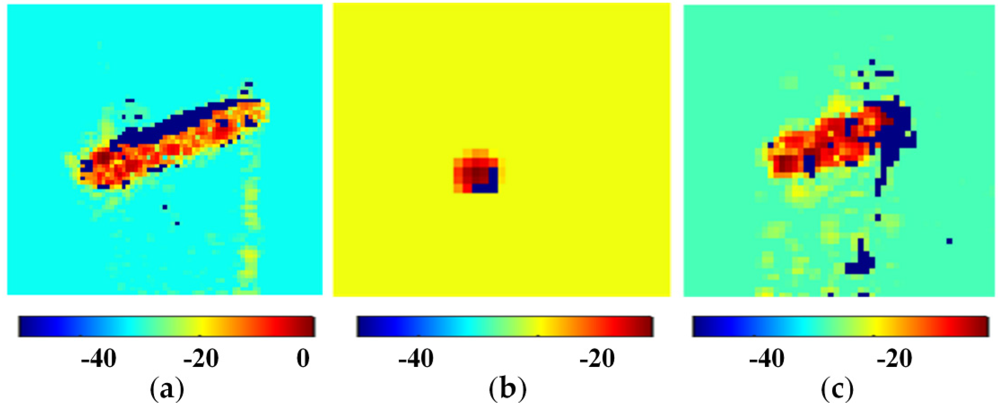
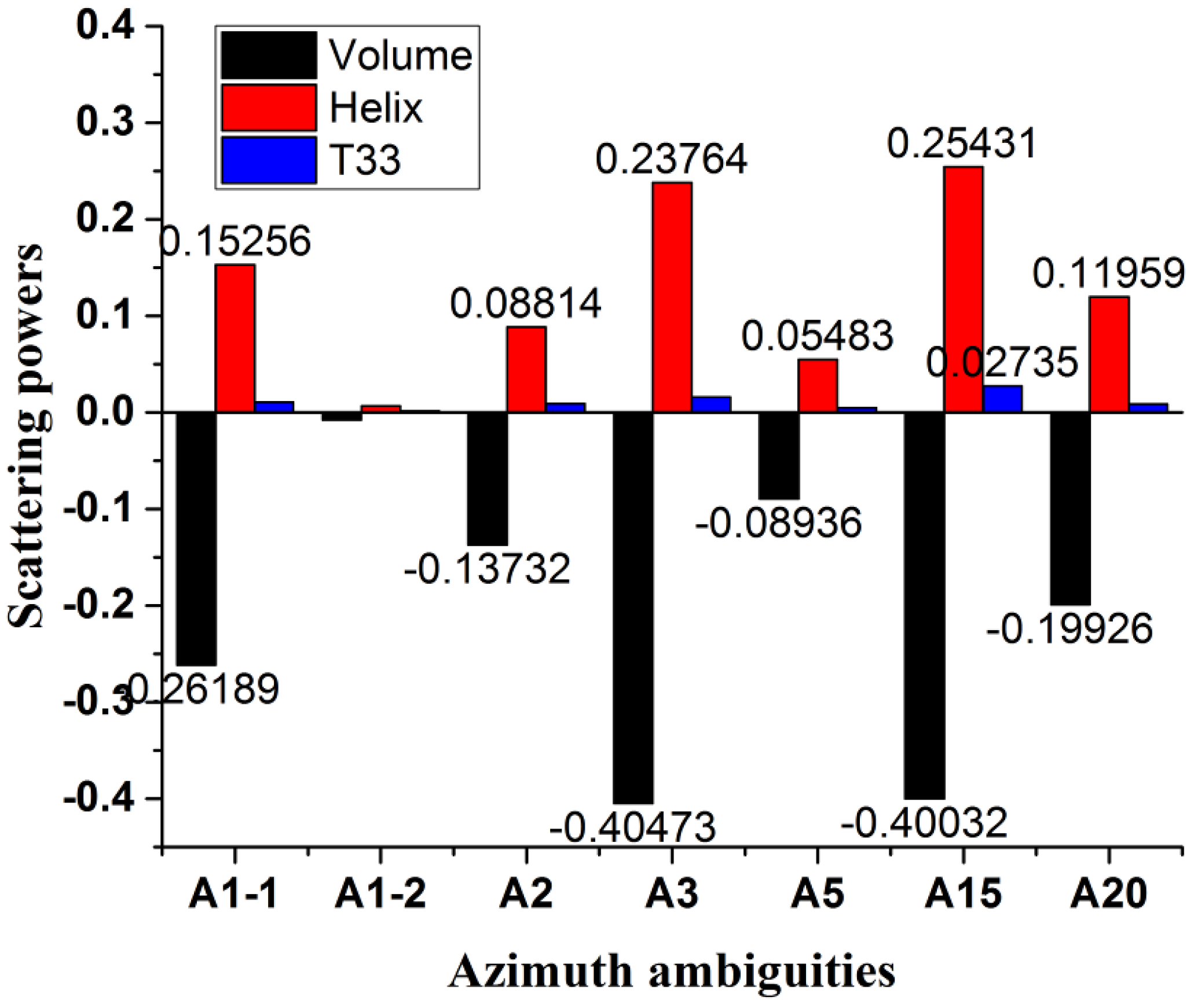
4.2. Different Polarimetric Scattering Characteristics between Ships and Azimuth Ambiguities

The size of the processing window or the number of ensemble averages plays an important role for accurate decomposition. If the number is too large, resolution of the decomposed image is lost, and the scattering characteristics are merged together. On the other hand, if the number is too small, the averaged quantities do not obey the theoretical second-order statistics. Thus, considering that the PolSAR data have been multilook-processed by nine-look in the azimuth direction, the window size for Yamaguchi decomposition was chosen to be 3 × 3 pixels for avoiding small ships to be smoothed severely in the decomposed results shown in Figure 3.
Figure 3. Yamaguchi decomposition results. (a) odd-bounce scattering; (b) double-bounce scattering; (c) volume scattering; and (d) helix scattering. All the powers are recalculated in decibels by 10 × 1og10(power + 1e−5).
Remotesensing 08 00074 g003
In order to obviously show the variation of mean scattering powers of each decomposition component across all targets and ambiguities with respect to the clutter power, we sampled all ships, ambiguities and their corresponding surrounding sea clutter, and statistically analyzed TCRs of ships and ambiguities, respectively. The statistical results are shown in Figure 4.
Figure 4. The variation of mean target-to-clutter ratio (TCR) of ships and ambiguities in each decomposition component. (a) odd-bounce scattering; (b) double-bounce scattering; (c) volume scattering; and (d) helix scattering.
Remotesensing 08 00074 g004
It is seen in Figure 3a,b that ships and their azimuth ambiguities both have strong odd-bounce scattering and double-bounce scattering, such as A11, A2, A3, A5, A15, and A20. From Figure 4a,b, there is no sharp distinction between ships and ambiguities. This means that azimuth ambiguities would be easily mistaken as ships with the odd- or double-bounce scattering.
Figure 3c and Figure 4c show that most azimuth ambiguities have low volume scattering power relative to ships but the scattering power of some ambiguities (e.g., A11, A3, and A15, etc.) are still close to some small ships (e.g., S11, S12, and S17, etc.) in the volume scattering. The residual ambiguities in the volume scattering power image will influence on small ship detection. That is, if only the volume scattering mechanism is utilized to detect ships by thresholding, the residual ambiguities also lead to false alarms or small ships will be missed.
According Figure 3d, it is shown that the scattering powers of azimuth ambiguities are almost equal to −50 dB, which were calculated by the expression 10 × 1og10(power + 1e−5). This means that azimuth ambiguities almost have zero helix scattering. Figure 4d also shows that there are clear differences between ships and the ambiguities. It is indicated that helix scattering can be potential to distinguish ships from azimuth ambiguities. Howerver, man-made objects orthogonal to radar illumination usually have no helix scattering [18]. Due to some physical factors (e.g., ship structure, and radar incidence angle, etc.), some parts of a ship orthogonal to radar look direction also have zero helix scattering (See Figure 3d). In this case, some ships in the helix scattering power image look incomplete, such as S3, S12, and S15. If the helix scattering power is directly utilized to detect ships, a complete ship in itself would become discontinuous in the detection result. In order to help recognize some parts of ships having fhlx ~= 0, we also zoomed in S3, S12, and S15 (See Figure 5a–c).
Figure 5. Zoom in S3, S12, and S15. (a) S3; (b) S12; and (c) S15. The powers are also calculated in decibels by 10 × 1og10(power + 1e−5).
Remotesensing 08 00074 g005
In addition, in order to explain the zero helix scattering powers generated from the negative volume scattering powers, we sampled all the powers of ambiguities from the helix and volume scattering derived from the original Yamaguchi decomposition [17] besides from T33. Figure 6 shows the statistical results.
Figure 6. The quantitative comparison among the helix and volume scattering powers from the original Yamaguchi decomposition [17] and T33 for azimuth ambiguities.
Remotesensing 08 00074 g006
As mentioned in Section 2, the maximum amplitude of the first ambiguity in SHV is always considerably smaller than that of the target image for zero velocity. In other words, the ambiguities have low 2<|SHV|2> (i.e., T33) relative to ships. Therefore, since fhlx in Equation (5) is constant, azimuth ambiguities usually have low volume scattering powers relative to ships. Moreover, by examining Equation (4), the helix scattering power fhlx is estimated by product of the cross-polarization SHV and double bounce scattering. As the above mention, the ambiguities usually have very strong odd- or double-bounce scattering powers. In this case, helix scattering power (fhlx) estimated by the produce of HV and double-bounce scattering, usually is larger than T33. By Figure 6, the powers of the helix scattering are much stronger than that of the T33 for azimuth ambiguities, which leads to the negative volume scattering powers. As mentioned in Section 4.1, in order to avoid negative volume scattering powers, the helix scattering powers have to be enforced as zero and then the volume scattering powers are recalculated.
Overall, the experimental results show that ambiguities accompanied with strong odd- or double-bounce scattering usually have low volume scattering and zero helix scattering by the modified Yamaguchi decomposition, which implies that the volume and helix scattering can be potential to distinguish ships from azimuth ambiguities.

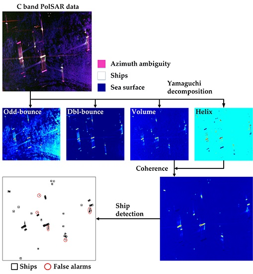
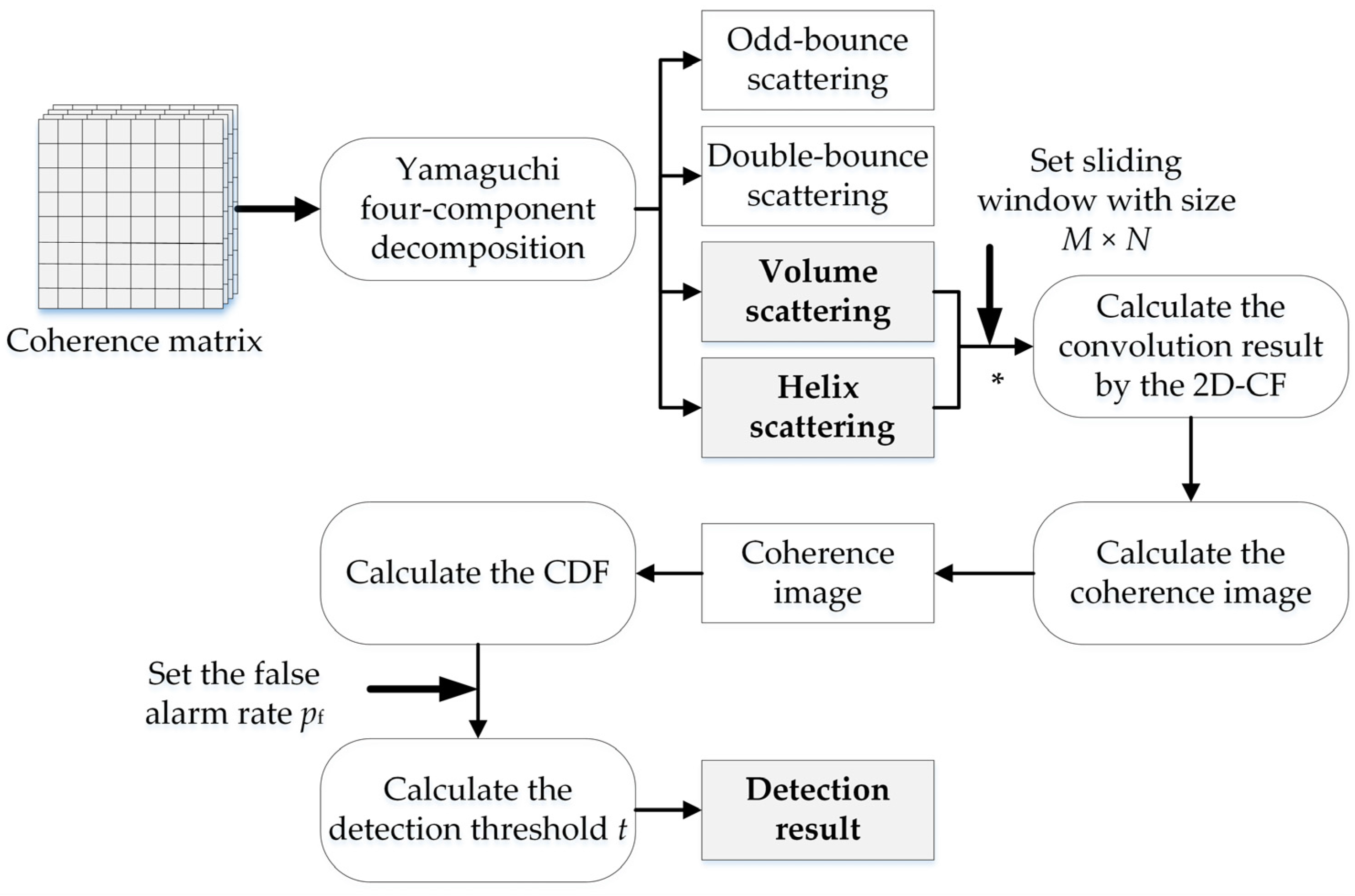
5. Ship Detection Method

As mentioned in the above section, azimuth ambiguities usually have lower volume scattering power than ships and the ambiguities almost have no helix scattering. However, sometimes residual ambiguities still exist in the volume scattering power and have close intensity to small ships. In this case, small ships will be missed or false alarms will also be produced by the ambiguities only using the volume scattering power for ship detection. Moreover, because of some physical factors, e.g., ship structure and radar incidence angle, some parts of a ship orthogonal to radar illumination may also have no helix scattering. It has been proved that it is beneficial to decrease the miss rate of small ships by increasing target-to-clutter ratio [14,22,23,24,25]. The two-dimensional convolution function (2D-CF) is often applied to enhance feature and filter image in digital image processing field. By the 2D-CF, there will appear a peak when two images have strong cross-correlation [24]. Thus, the 2D-CF is introduced to get the coherence image of the volume and helix scattering for high detection precision. The coherence image is calculated by the 2D-CF with sliding window of size M × N on both the intensity images of the volume and helix scattering.
The 2D-CF is defined as:
F ( x , y ) = f * g = m = 0 M 1 n = 0 N 1 f ( m , n ) g ( x m , y n )
where 0 ≤ x < 2M − 1, 0 ≤ y < 2N − 1; the asterisk (*) is convolution operator; f and g stand for the volume scattering power and the helix scattering power, respectively.
Then the coherence image (Rc) is calculated by:
R c ( x , y ) = x = 0 2 M 1 y = 0 2 N 1 F ( x , y ) / ( ( 2 M 1 ) ( 2 N 1 ) )
When we get the coherence image, ships then can be detected by imposing a global threshold t on it. If pixel values of the coherence image exceed t they will be regarded as ships, otherwise, as background clutters. The threshold t can be evaluated by Equation (8):
p f = t f ( x ) d x = 1 F ( t )
where pf is the given false alarm rate. f(∙) and F(∙) are the probability density function (PDF) and its corresponding cumulative distribution function (CDF) of the coherence image, respectively.
If the CDF F(∙) is known, the global threshold t can be estimated with the given pf by Equation (8). And F(∙) can be estimated in the following way. Suppose that there are K pixels in the image, the pixel values are arranged in ascending order. Thus, we have a set of pixel values {x1, x2, …, xK} with x1x2 ≤ … ≤ xK. Then F(xk), k = 1, 2, …, K, is estimated by:
F ( x k ) = Num ( { i | x i x k , i { 1 , 2 , , K } } ) K
where Num(∙) counts the number of elements of a set.
To sum up, the proposed detection procedures are shown in Figure 7, and their corresponding major steps are summarized as follows:
(1) Polarimetric target decomposition for PolSAR data by Yamaguchi method to get four scattering components, i.e., odd-bounce scattering, double-bounce scattering, volume scattering, and helix scattering.
(2) To set sliding window with size of M × N for calculating the convolution of the volume and helix scattering powers by the 2D-CF.
(3) To compute the coherence image using the calculated convolution result by Equation (7).
(4) To estimate the CDF F(∙) of the coherence image by Equation (9).
(5) To determine the threshold t by Equation (8) with the given false alarm rate pf and the calculated CDF.
(6) To detect ships by imposing the threshold t on the coherence image. Pixels whose values exceed t are regarded as ships and, otherwise, as background clutters.
Figure 7. Flowchart of the proposed ship detection method.
Remotesensing 08 00074 g007

6. Exprimental Results and Discussion

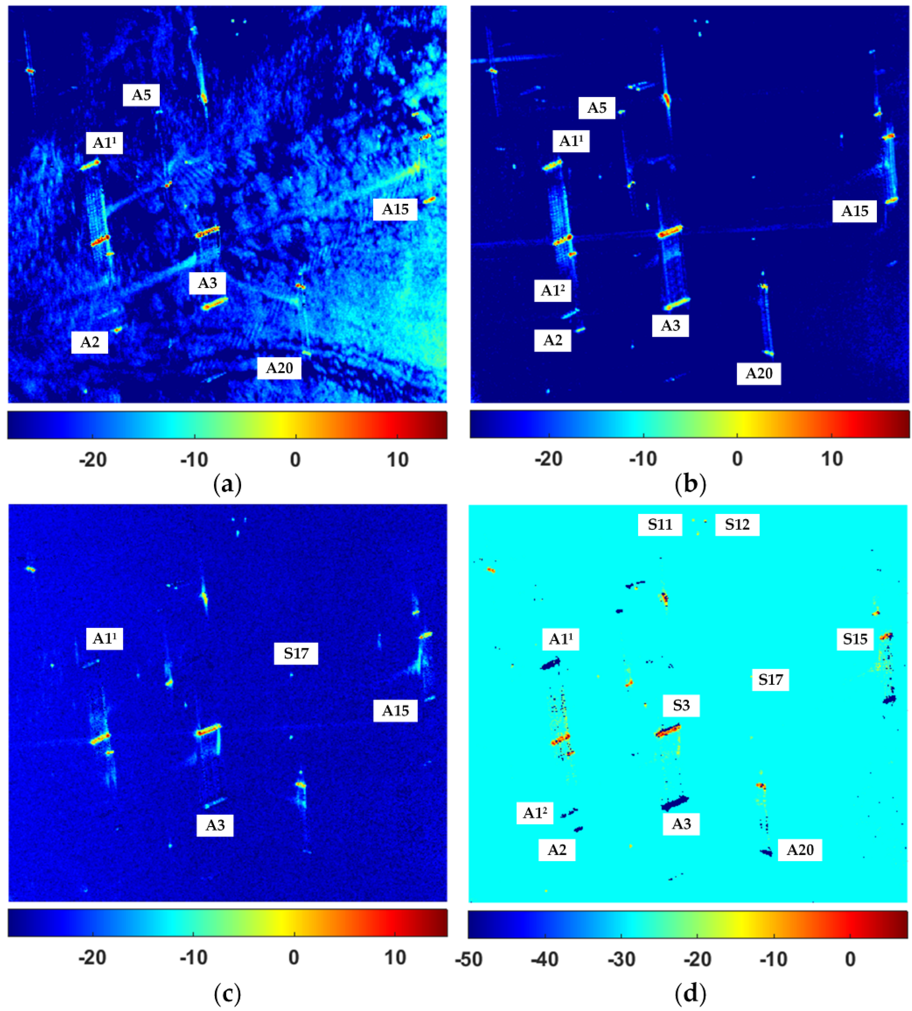
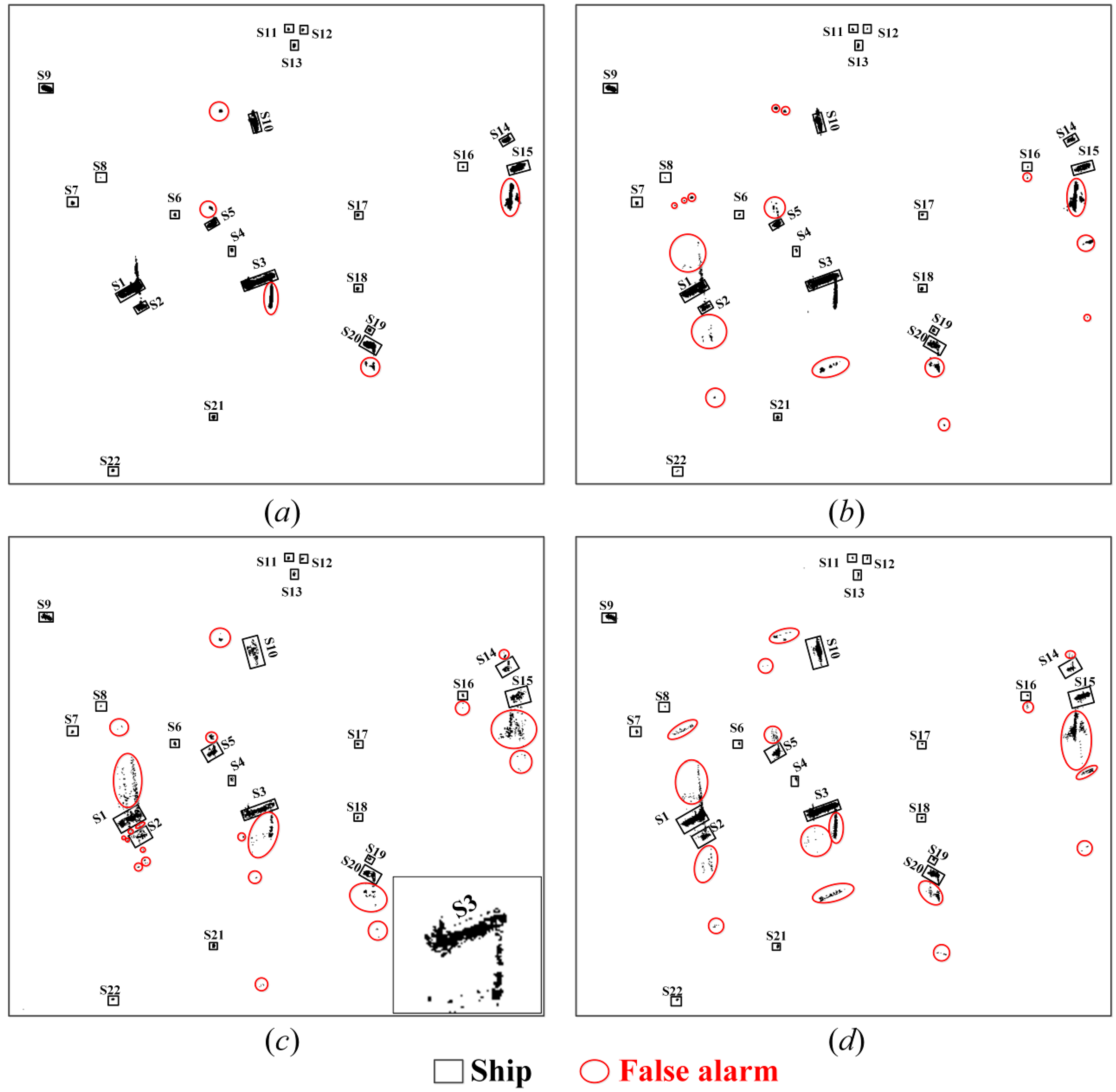
6.1. Algorithm Verification

According to the proposed ship detection procedures, after Yamaguchi decompistion for the C-band PolSAR data, the coherence image shown in Figure 8 was calculated based on cross-correlation between the volume and helix scattering powers by the 2D-CF with the sliding window of size 3 × 3 pixels. According to Figure 3c,d, there are some residuary ambiguities in the volume scattering image but no ambiguities in the helix scattering image correspondingly. In this case, the cross-correlation of the overlap between both the scattering powers is low by the 2D-CF. On the contrary, ships colocated in both the volume and helix scattering images have strong correlation. Thus, the convolution value of the continuously changing ocean surface and azimuth ambiguities decreases relative to initial data, while that of ships increases. In other words, the residual ambiguities can be eliminated effectively and the target-to-clutter ratio can be improved to some degree. Moreover, some parts of ships having zero helix scattering powers also can be smoothed by the 2D-CF. By comparing Figure 8 with Figure 2 and Figure 3a–d, it is shown that azimuth ambiguities are removed effectively and ships almost can maintain their complete structure after the coherence. The enlarged images of S3, S12, and S15 from the coherence image are also shown in Figure 9. By comparing Figure 5 including S3, S12, and S15 from the helix scattering component with Figure 9, it is obviously shown that the discontinuous ships in the helix scattering power almost become perfect after the coherence.
Figure 8. The coherence image derived from cross-correlation between the volume and helix scattering. And the coherence result is also recalculated in decibels by 10 × 1og10(power + 1e−5).
Remotesensing 08 00074 g008
Figure 9. Zoom in S3, S12, and S15 after the coherence. (a) S3; (b) S12; and (c) S15. The powers are also calculated in decibels by 10 × 1og10(power + 1e−5).
Remotesensing 08 00074 g009
Next, the CDF of the coherence image was calculated by Equation (9). Then, the global threshold t was calculated as −35.75 dB by Equation (8) with the given false alarm rate pf (setting as 0.006). Finally, the calculated threshold t was applied to the coherence image for ships detection, and then the detection result is shown in Figure 10a. The result shows that ships are all discriminated from the azimuth ambiguities, which proves the effectiveness of the new method. However, there are some false alarms labeled by the red ellipses, which are mainly caused by ship wakes with much different scattering characteristics.

6.2. Discussion

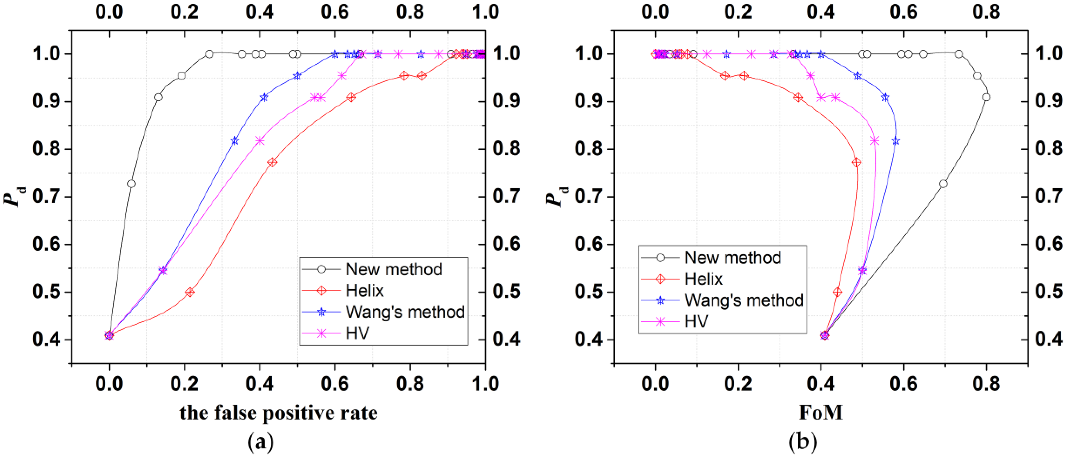
6.2.1. The Comparison of Detection Performance

In order to further validate the performance of the proposed method, Wang’s algorithm [2] was also applied to the C-band PolSAR data. Moreover, the intensity images of the helix scattering mechanism and the T33 are also separately applied for ship detection. Their best detection results are shown in Figure 10b–d, respectively. By comparing Figure 10a–d, it is clearly shown that all ships can be detected by the methods but the detection result from our method has the least false alarms than other three methods. With respect to our method, most of the false alarms in the detection results from Wang’s method and T33 are generated from residuary azimuth ambiguities besides some false alarms derived from ship wakes. Similarly, ship wakes also induce most false alarms in the detection result by the helix scattering power and some detected ships in the detection result look incomplete or contain holes (e.g., the enlarged S3 in Figure 10c).
Figure 10. Various ship detection results. (a) The detection result by the new method; (b) the detection result by Wang’s method; (c) the detection result by the helix scattering power; and (d) the detection result by T33.
Remotesensing 08 00074 g010
Then the detection probability Pd and the figure of merit (FoM) [3,26], defined as Equation (10), were selected for quantitative comparison among all the methods.
P d = N td / N gt        FoM = N td / ( N fa + N gt )
where Ntd is the number of targets detected correctly in the detection result; Nfa is the number of false alarms; Ngt is the number of ground truth targets.
It is known that the greater the Pd and FoM, the higher the detection precision and Figure 11a,b obviously shows that the new method always provides better performance than the other methods.
Figure 11. The quantitative comparison among the methods. (a) ROC plots for the different detectors; and (b) the quantitative comparison among the methods by FoM vs. Pd.
Remotesensing 08 00074 g011

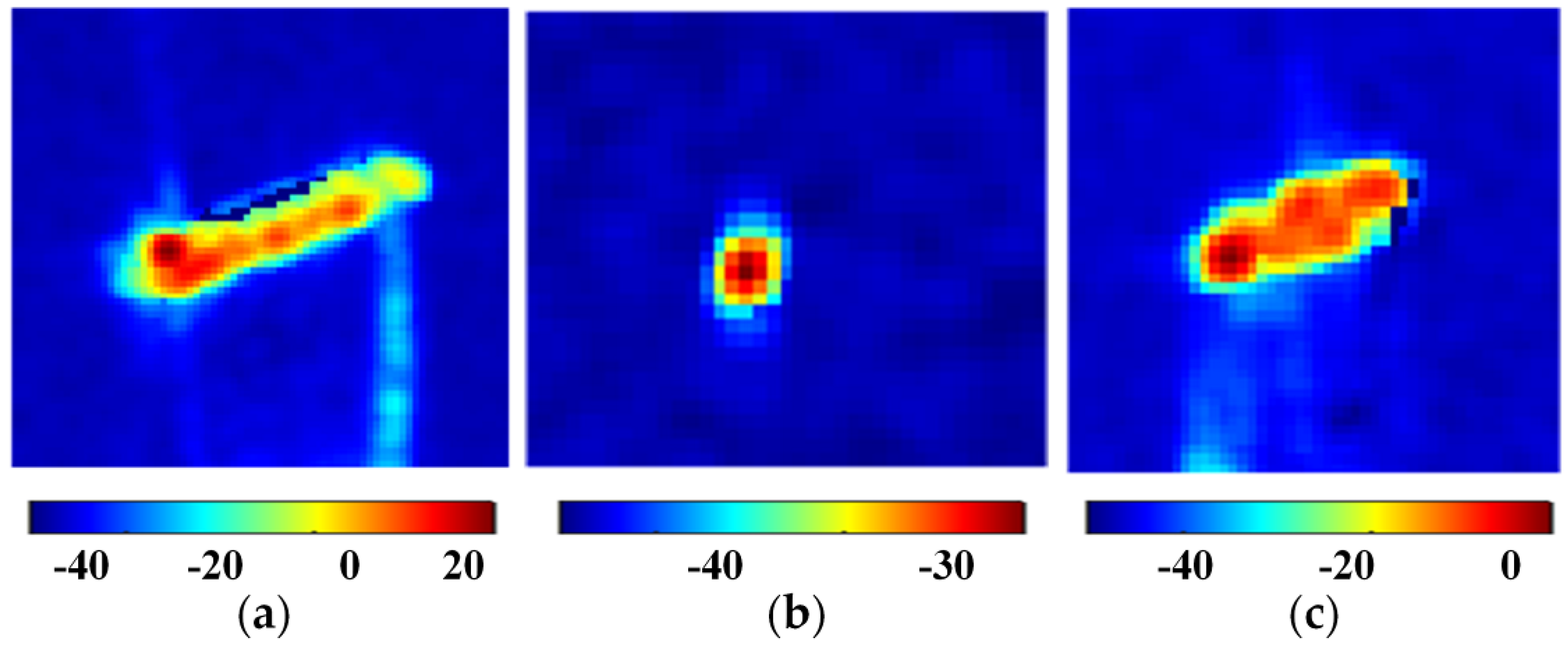
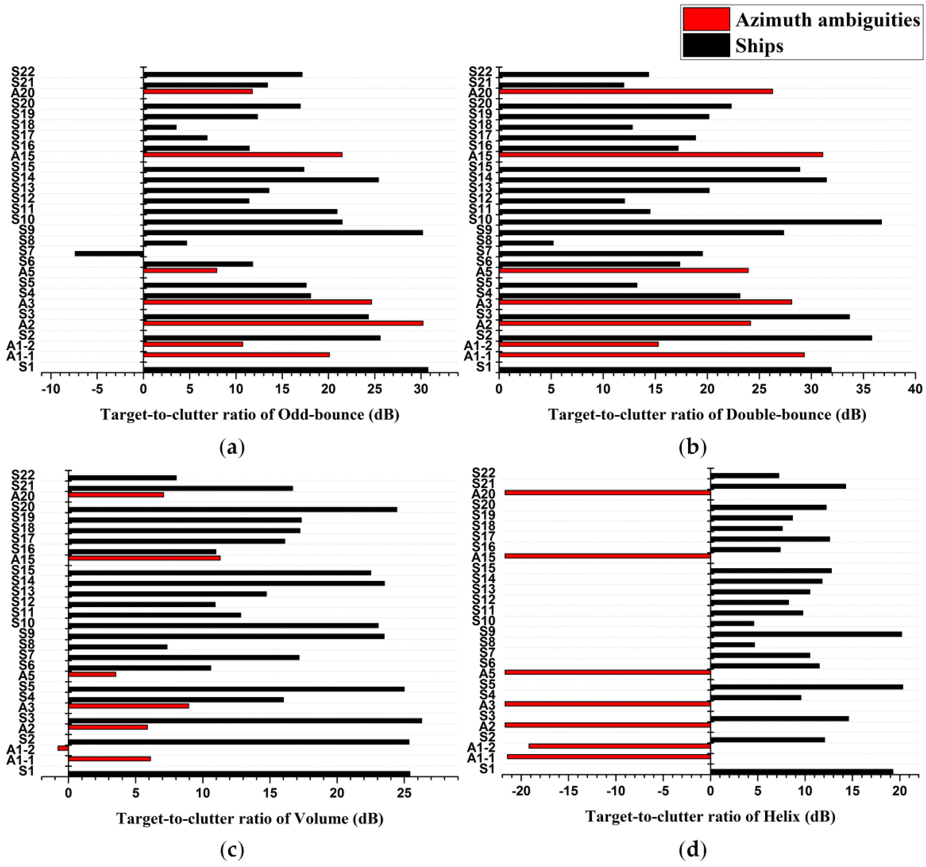
6.2.2. The Enhancement of TCR by Cross-Correlation between Volume and Helix Scattering

In this section, the four local areas were selected (See Figure 2) for the quantitatively illustration that the TCR can be enhanced and the residual ambiguities in volume scattering can be further suppressed based on cross-correlation between volume and helix scattering by 2D-CF. The test area A contains small ships (S7 and S8), big ships (S1 and S2), and the ambiguities (A11 and A2). The test area B contains small ship S4, big ship S3, and its corresponding azimuth ambiguity A3. The test area C contains small ships (S18 and S19), and big ship S20,with its ambiguity A20. The test area D contains small ship S16, big ships (S14 and S15) and the ambiguity A15. Figure 12 obviously displays that the differences of TCRs of ships and ambiguities among the volume scattering, the helix scattering, the coherence results, and the third eigenvalues from the selected four test areas.
According to Figure 12, there still exist some residual ambiguities in the volume scattering and the third eigenvalue. After the cross-correlation between the volume and helix scattering, the residual ambiguities are suppressed and the TCR is increased to some extent in terms of the respective legend bar of the volume scattering, the helix scattering, the third eigenvalue, and the coherence image.
Let us take the local area B for instance as shown in Figure 12. It can be seen that the ship S3 still has its azimuth ambiguity A3, whose intensity is close to the small ship S4 in the volume scattering, while the helix scattering of ambiguity A3 is very low relative to ships and even to be zero. Furthermore, some parts of ship S3 and S4 also have zero helix scattering power so that the ships with holes look discontinuous. Then, their coherence result shows that the holes in ships have been smoothed so that ships all become complete and continuous, and the residual ambiguity A3 has been removed. Moreover, according to the corresponding legend, the magnitude ranges of the volume scattering, helix scattering, the coherence result and the third eigenvalue are −28.4–15.2 (dB), −50.0–6.6 (dB), −50.0–23.8 (dB) and −50.0–4.0 (dB), respectively. By comparing among these figures, it is obviously shown that the target-to-clutter ratio can be increased based on cross-correlation between volume and helix scattering by 2D-CF.
Furthermore, we took some samples, i.e., some small ships and their surrounding sea clutter, from the volume power (Vol), the helix scattering power (Hlx), and the coherence image (Coh), to further quantitatively validate whether the target-to-clutter ratio can be increased by the 2D-CF. See Table 2 for more details about the statistical analysis results. By Table 2, the averaged target-to-clutter ratio in the coherence image is about 20.86 dB, which is increased by 8.13 dB and 8.53 dB relative to the volume and helix scattering, respectively.
In short, it is demonstrated that the new method not only suppresses the azimuth ambiguity well but also increases the target-to-clutter ratio to some extent, which benefits ship detection with high accuracy.
Figure 12. The quantitative comparison between our method and Wang’s method. From the top down, each row corresponds to the test area A, B, C, and D, respectively. From left to right, each column corresponds to the volume scattering, the helix scattering, the coherence result derived from cross-correlation between the volume and helix scattering, and the third eigenvalue derived from Cloude decomposition, respectively. The scattering powers and the coherence intensity are all calculated in decibels (dB) by 10 × 1og10(power + 1e−5).
Remotesensing 08 00074 g012
Table 2. Statistical analysis of target-to-clutter ratio within the volume, helix, and coherence image by sampling (unit: dB).
Ship IDShipSurrounding SeaTarget-to-Clutter Ratio
VolHlxCohVolHlxCohVolHlxCoh
S6−14.927−17.351−28.868−24.866−28.198−45.7319.93910.84716.863
S7−6.963−17.587−21.542−23.430−28.261−44.75516.46710.67423.213
S11−12.987−17.834−27.876−25.516−28.155−46.01112.52910.32118.135
S12−17.526−16.567−30.626−25.847−28.353−46.3678.32111.78615.741
S17−10.810−15.460−23.688−25.691−28.239−46.23214.88112.77922.544
S19−7.813−16.846−21.735−25.624−28.188−46.02517.81111.34224.290
S21−7.465−10.916−15.956−25.231−28.187−45.89517.76617.27129.939
S22−20.065−14.634−29.222−24.219−28.229−45.3674.15413.59516.145

7. Conclusions

In this paper the intrinsic characteristics of ships and azimuth ambiguities in PolSAR data are described briefly; that is, the first ambiguities usually have strong odd- or double-bounce scattering powers and the maximum amplitude of the first ambiguity in SHV is always considerably smaller than that of the corresponding target for zero or high velocity. Based on this property, this paper examined that azimuth ambiguities usually have lower volume scattering power than ships and the ambiguities almost have no helix scattering by Yamaguchi decomposition. Then, a new general ship detection method was proposed for high-precision ship detection using cross-correlation between the two scattering mechanisms. It is proved that the proposed method can avoid false alarms caused by azimuth ambiguities, and at the same time can enhance target-to-clutter ratio for reducing the miss detection rate of small ships. Since Yamaguchi decomposition can work effectively with the Sinclair matrix (S2), the coherence matrix (T3), and the covariance matrix (C3), this method is also suitable for the matrix S2 of PolSAR data in addition to the matrices T3 and C3. It is indicated that the new method is simple and more practical than previous methods.
Although the new method can detect ships effectively, there also exist some false alarms, mainly caused by ship wakes with much different scattering mechanisms from sea clutter. Therefore, we will focus on analysis of the scattering behavior of ship wakes and aim to minimize their impacts on ship detection in our future research. Moreover, we will further validate the effectiveness of the proposed algorithm in a range of sea conditions by using various PolSAR data with ground truth data. In particular, we will examine the helix and volume scattering powers of azimuth ambiguities with various across-track velocity of ships.

Acknowledgments

The study was financially supported by the Special Fund by Surveying & Mapping and Geoinformation Research in the Public Interest (201412002) and the Special Fund by Surveying & Mapping and Geoinformation Research in the Public Interest (201412010). And I would like to thank the website (http://airsar.asf.alaska.edu/) for providing the AIRSAR data for free download.

Author Contributions

Jujie Wei is responsible for the design of the study, experimental data collection and processing, resultant analysis, and preparation of the manuscript. Jixian Zhang, Guoman Huang and Zheng Zhao are responsible for the technical support of the manuscript.

Conflicts of Interest

The authors declare no conflict of interest.

References

  1. Curlander, J.C.; Mcdonough, R.N. Synthetic Aperture Radar: Systems and Signal Processing; Wiley-Interscience: New York, NY, USA, 1991. [Google Scholar]
  2. Wang, C.; Wang, Y.; Liao, M. Removal of azimuth ambiguities and detection of a ship: Using polarimetric airborne C-band SAR images. Int. J. Remote Sens. 2012, 33, 3197–3210. [Google Scholar] [CrossRef]
  3. Wei, J.J.; Li, P.X.; Yang, J.; Zhang, J.; Lang, F. A new automatic ship detection method using L-band polarimetric SAR imagery. IEEE J. Sel. Top. Appl. Earth Observ. 2014, 7, 1383–1393. [Google Scholar]
  4. Crisp, D.J. The State-of the Art in Ship Detection in Synthetic Aperture Radar Imagery; DSTO Information Sciences Laboratory: Edinburgh, Australia, 2004. [Google Scholar]
  5. Moreira, A. Suppressing the azimuth ambiguities in synthetic aperture radar images. IEEE Trans. Geosci. Remote Sens. 1993, 31, 885–895. [Google Scholar] [CrossRef]
  6. Monti Guarnieri, A. Adaptive removal of azimuth ambiguities in SAR images. IEEE Trans. Geosci. Remote Sens. 2005, 43, 625–633. [Google Scholar] [CrossRef]
  7. Di Martino, G.; Iodice, A.; Riccio, D.; Ruello, G. Filtering of azimuth ambiguity in stripmap synthetic aperture radar images. IEEE J. Sel. Top. Appl. Earth Observ. 2014, 7, 3967–3978. [Google Scholar] [CrossRef]
  8. Liu, C. Effects of target motion on polarimetric SAR images. Can. J. Remote Sens. 2006, 32, 51–64. [Google Scholar] [CrossRef]
  9. Liu, C. Time-frequency analysis of PolSAR moving target data. Can. J. Remote Sens. 2007, 33, 237–249. [Google Scholar] [CrossRef]
  10. Liu, C.; Gierull, C.H. A new application for PolSAR imagery in the field of moving target indication/ship detection. IEEE Trans. Geosci. Remote Sens. 2007, 45, 3426–3436. [Google Scholar] [CrossRef]
  11. Velotto, D.; Soccorsi, M.; Lehner, S. Azimuth ambiguities removal for ship detection using full polarimetric X-band SAR data. In Proceedings of the 2012 International Geoscience Remote Sensing Symposium (IGARSS), Munich, Germany, 22–27 July 2012; pp. 7621–7624.
  12. Velotto, D.; Soccorsi, M.; Lehner, S. Azimuth ambiguities removal for ship detection using full polarimetric X-band SAR data. IEEE Trans. Geosci. Remote Sens. 2014, 52, 76–88. [Google Scholar] [CrossRef]
  13. Lee, J.S.; Pottier, E. Polarimetric Radar Imaging: From Basics to Applications; CRC Pressl Llc: Boca Raton, FL, USA, 2009. [Google Scholar]
  14. Souyris, J.C.; Henry, C.; Adragna, F. On the use of complex SAR image spectral analysis for target detection: Assessment of polarimetry. IEEE Trans. Geosci. Remote Sens. 2003, 41, 2725–2734. [Google Scholar] [CrossRef]
  15. Hwang, S.I.; Ouchi, K. On a novel approach using MLCC and CFAR for the improvement of ship detection by Synthetic Aperture Radar. IEEE Geosci. Remote Sens. Lett. 2010, 7, 391–395. [Google Scholar] [CrossRef]
  16. Freeman, A. The effects of noise on polarimetric SAR data. In Proceedings of the 1993 International Geoscience Remote Sensing Symposium (IGARSS), Tokyo, Japan, 18–21 August 1993; Volume 2, pp. 799–802.
  17. Yamaguchi, Y.; Moriyama, T.; Ishido, M.; Yamada, H. Four-component scattering model for polarimetric SAR image decomposition. IEEE Trans. Geosci. Remote Sens. 2005, 43, 1699–1706. [Google Scholar] [CrossRef]
  18. Yajima, Y.; Yamaguchi, Y.; Sato, R.; Yamada, H. POLSAR image analysis of wetlands using a modified four-component scattering power decomposition. IEEE Trans. Geosci. Remote Sens. 2008, 46, 1667–1673. [Google Scholar] [CrossRef]
  19. Yamaguchi, Y.; Sato, A.; Boerner, W.M.; Sato, R. Four-component scattering power decomposition with rotation of coherency matrix. IEEE Trans. Geosci. Remote Sens. 2011, 49, 2251–2258. [Google Scholar] [CrossRef]
  20. Sato, A.; Yamaguchi, Y.; Singh, G.; Sang-Eun, P. Four-component scattering power decomposition with extended volume scattering model. IEEE Geosci. Remote Sens. Lett. 2012, 9, 166–170. [Google Scholar] [CrossRef]
  21. Singh, G.; Yamaguchi, Y.; Park, S.E. General four-component scattering power decomposition with unitary transformation of coherency matrix. IEEE Trans. Geosci. Remote Sens. 2013, 51, 3014–3022. [Google Scholar] [CrossRef]
  22. Arnaud, A. Ship detection by SAR interferometry. In Proceedings of the 1999 International Geoscience Remote Sensing Symposium (IGARSS), Hamburg, Germany, 28 June–2 July 1999; pp. 2616–2618.
  23. Ouchi, K.; Tamaki, S.; Yaguchi, H.; Iehara, M. Ship detection based on coherence images derived from cross correlation of multilook SAR images. IEEE Geosci. Remote Sens. Lett. 2004, 1, 184–187. [Google Scholar] [CrossRef]
  24. Li, H.Y.; He, Y.J.; Wang, W.G. Improving ship detection with polarimetric SAR based on convolution between co-polarization channels. Sensors 2009, 9, 1221–1236. [Google Scholar] [CrossRef] [PubMed]
  25. Wang, Y.; Liu, H. A hierarchical ship detection scheme for high-resolution SAR images. IEEE Trans. Geosci. Remote Sens. 2012, 50, 4173–4184. [Google Scholar]
  26. Paes, R.L.; Lorenzzetti, J.A.; Gherardi, D.F.M. Ship detection using TerraSAR-X images in the campos basin (Brazil). IEEE Geosci. Remote Sens. Lett. 2010, 7, 545–548. [Google Scholar] [CrossRef]

