Article

Evaluation of ASTER-Like Daily Land Surface Temperature by Fusing ASTER and MODIS Data during the HiWATER-MUSOEXE

1
Beijing Research Center for Information Technology in Agriculture, Beijing Academy of Agriculture and Forestry Sciences, Beijing 100097, China
2
School of Geography, South China Normal University, Guangzhou, Guangdong 510631, China
3
Center for Urban and Environmental Change, Department of Earth and Environmental Systems, Indiana State University, Terre Haute, IN 47809, USA
4
School of Geosciences, University of South Florida, Tampa, FL 33620, USA
5
Hydrology and Remote Sensing Laboratory, Agricultural Research Service, US Department of Agriculture, Beltsville, MD 20705, USA
6
State Key Laboratory of Remote Sensing Science, Institute of Remote Sensing and Digital Earth, Chinese Academy of Sciences, Beijing 100010, China
*
Author to whom correspondence should be addressed.
Remote Sens. 2016, 8(1), 75; https://doi.org/10.3390/rs8010075
Submission received: 12 November 2015 / Revised: 23 December 2015 / Accepted: 14 January 2016 / Published: 21 January 2016

Abstract

:
Land surface temperature (LST) is an important parameter that is highly responsive to surface energy fluxes and has become valuable to many disciplines. However, it is difficult to acquire satellite LSTs with both high spatial and temporal resolutions due to tradeoffs between them. Thus, various algorithms/models have been developed to enhance the spatial or the temporal resolution of thermal infrared (TIR) data or LST, but rarely both. The Spatial and Temporal Adaptive Reflectance Fusion Model (STARFM) is the widely-used data fusion algorithm for Landsat and MODIS imagery to produce Landsat-like surface reflectance. In order to extend the STARFM application over heterogeneous areas, an enhanced STARFM (ESTARFM) approach was proposed by introducing a conversion coefficient and the spectral unmixing theory. The aim of this study is to conduct a comprehensive evaluation of the ESTARFM algorithm for generating ASTER-like daily LST by three approaches: simulated data, ground measurements and remote sensing products, respectively. The datasets of LST ground measurements, MODIS, and ASTER images were collected in an arid region of Northwest China during the first thematic HiWATER-Multi-Scale Observation Experiment on Evapotranspiration (MUSOEXE) over heterogeneous land surfaces in 2012 from May to September. Firstly, the results of the simulation test indicated that ESTARFM could accurately predict background with temperature variations, even coordinating with small ground objects and linear ground objects. Secondly, four temporal ASTER and MODIS data fusion LSTs (i.e., predicted ASTER-like LST products) were highly consistent with ASTER LST products. Here, the four correlation coefficients were greater than 0.92, root mean square error (RMSE) reached about 2 K and mean absolute error (MAE) ranged from 1.32 K to 1.73 K. Finally, the results of the ground measurement validation indicated that the overall accuracy was high (R2 = 0.92, RMSE = 0.77 K), and the ESTARFM algorithm is a highly recommended method to assemble time series images at ASTER spatial resolution and MODIS temporal resolution due to LST estimation error less than 1 K. However, the ESTARFM method is also limited in predicting LST changes that have not been recorded in MODIS and/or ASTER pixels.

Graphical Abstract

1. Introduction

Land-surface temperature (LST) is a key parameter of the physics of land-surface processes at the regional and global scales, and it includes combined effects of all surface–atmosphere interactions and energy fluxes [1,2,3,4,5,6,7]. Due to the strong heterogeneity of land surface characteristics such as vegetation, soil, water, and topography [8,9], LST changes rapidly over both spatial and temporal scales [10,11,12]. In practice, the spatial and temporal resolution requirements of satellite-derived surface temperature data for agricultural applications are estimated to be about 40 m and 1 day (revisit time), respectively [13]. Therefore, high-resolution LST measurements obtained with remote sensing approaches are highly desired. However, acquiring satellite images with high temporal and spatial resolutions remains extremely difficult due to tradeoffs between both resolutions. For example, the temporal frequency of the Moderate Resolution Imaging Spectrometer (MODIS, low-spatial/high-temporal resolution sensor) with a 1-km spatial resolution is greater than one visit per day [14,15]. In contrast, the temporal frequency of the Advanced Spaceborne Thermal Emission and Reflection Radiometer (ASTER, high-spatial/low-temporal resolution sensor) with a 90-m spatial resolution is greater than 15 days [16,17].
To bridge the gap between the low spatial resolution of available thermal data and the high spatial resolution required over agricultural areas, one may disaggregate low-spatial-resolution thermal data at high-temporal frequencies. Existing techniques have been reported in interdisciplinary literature, including image/data fusion [18,19,20,21,22,23,24,25,26,27,28], spatial sharpening [15,29,30,31,32,33], downscaling and disaggregation [3,10,17,34,35,36] and their comparisons [37,38,39,40]. Various methods of LST downscaling can be broadly grouped into physical and statistical categories. For statistical methods, a relationship between a vegetation index/variable (e.g., the Normalized Difference Vegetation Index, NDVI) and radiometric surface temperature can be addressed by a linear or nonlinear function. Due to the fact that vegetation indices (VIs) are often available at a finer pixel resolution than LST, there is a potential to make use of the VI–LST relationship to derive LST at the VI pixel resolution [17]. Physical downscaling uses modulation methods, which take a thermal pixel as a block and distribute its LST or thermal radiance into finer pixels corresponding to its shorter wavebands. However, the isothermal assumption that underpins various modulation methods may cause some errors, especially in vegetated areas that are composed of a mixture of different temperature components [10]. To our knowledge, many disaggregation methods do not yield ideal results in areas where vegetation cover is mixed with other land cover types, especially those areas covered with mixture of bare soil, water, and impervious components [3]. In fact, many bare lands, lakes or rivers, and villages or towns are irregular in shape and have variable sizes and distributions in agricultural fields, which are typical features of agricultural landscapes in China [41,42]. Although thermal downscaling methods can produce LST data with a relatively high spatial resolution in the order of 10–100 m, they do not simultaneously increase the temporal resolution of the sensor.
The Spatial and Temporal Adaptive Reflectance Fusion Model (STARFM) [18] is perhaps the most widely used data fusion algorithm for Landsat and MODIS imagery [19,20,21,22,23,24,25,26,27,28,37,39,40]. It is one of the few data fusion methods that result in synthetic Landsat-like surface reflectance [21,40,43]. The basic assumption underlying the method is that the surface reflectance on a predicted date can be estimated as a weighted sum of spectrally similar neighborhood information from both Landsat and MODIS reflectances on observation dates (close to the predicted date). In fact, STARFM integrates daily information from MODIS with periodic Landsat data to interpolate surface reflectance at the Landsat resolution of 30 m on a daily basis [19,20,24]. STARFM relies on temporal information from pure, homogeneous patches of land cover at the MODIS pixel scale. Simulations and predictions based on actual Landsat and MODIS images show that STARFM can accurately predict reflectance if these coarse-resolution homogeneous pixels exist [18]. However, the prediction results degrade somewhat when used on heterogeneous fine-grained landscapes, including small-scale agriculture [18,19]. Zhu et al. (2010) [20] developed an enhanced STARFM (ESTARFM) approach for application in a heterogeneous area by introducing a conversion coefficient and a spectral unmixing theory to the fusion model. However, as an essential part of the important work before using ESTARFM algorithm for generating high spatial-temporal LST products, an evaluation should be conducted over heterogeneous areas. The ESTARFM algorithm requires at least two pairs of fine- and coarse-resolution images acquired at the same date and a set of coarse-resolution images for desired prediction dates. Therefore, it should be evaluated how the selection of imagery pairs affects the performance of the data fusion algorithm.
Although ESTARFM was originally designed to fuse shortwave reflectance data from MODIS and Landsat to create daily reflectance, it is also greatly beneficial for the prediction of high spatial-temporal resolution thermal maps. Recently, Weng et al. (2014) [24] improved the STARFM method for predicting thermal radiance and LST data by considering the annual temperature cycle (ATC) over a heterogeneous urban area. This technique, the Spatio-temporal Adaptive Data Fusion Algorithm (SADFAT), blends Landsat and MODIS data to generate synthetic Landsat-like daily surface thermal data. They found that the prediction accuracy for the whole study area ranged from 1.3 K to 2 K [24]. Yang et al. (2015) [28] used ground measured temperature to evaluate the ESTARFM with a few temporal images. Therefore, based on our knowledge, most disaggregation methods for remotely sensed surface temperature were tested with only simulated data, or remote sensing products, or ground measurements. Therefore, these methods need a comprehensive evaluation and validation from three levels: simulation, remote sensing data, and ground observation.
The objective of this study was to evaluate the performance of the ESTARFM algorithm in retrieving LSTs using simulated data and coordination with ground measurements, MODIS, and ASTER data. All ground measurements and remote sensing data were collected in an arid region of Northwest China during the first thematic Multi-Scale Observation Experiment on Evapotranspiration (MUSOEXE) over heterogeneous land surfaces in 2012 [44], as a part of the Heihe Watershed Allied Telemetry Experimental Research (HiWATER) [45]. Following a brief introduction to the ground LST measurements collected in the HiWATER experiment, the satellite data used in this study is presented. The theoretical basis and application of the ESTARFM algorithm method are discussed in Section 3. The evaluation results from simulation, ground measurements and ASTER LST products are presented in Section 4. Finally, the discussion and conclusions of this study are summarized in Section 5 and Section 6, respectively.

2. Experimental Data

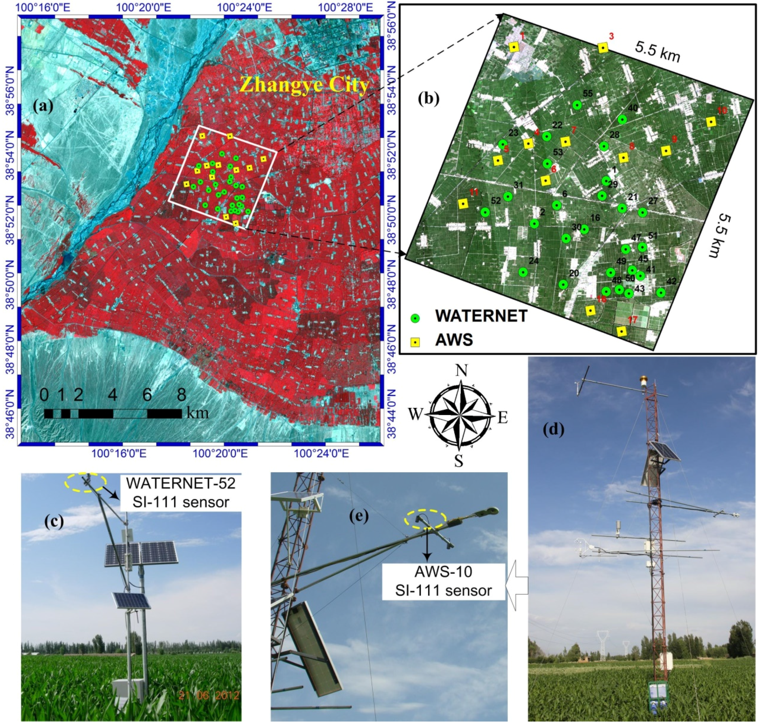
2.1. HiWATER-MUSOEXE Experiment

The HiWATER program was designed as a comprehensive ecohydrologic experiment and was based on the diverse needs of the interdisciplinary areas of the research plan and existing observation infrastructures in the Heihe River Basin [45]. The coordinate range of the study area is between 97.1°E–102.0°E and 37.7°N–42.7°N. The first thematic experiment launched in HiWATER was the HiWATER-MUSOEXE, which involved a flux observation matrix in the middle reach of a natural oasis area of the Heihe River Basin between May and September 2012 [44]. The HiWATER-MUSOEXE consisted of two nested matrices: one large experimental area (30 × 30 km) and one core experimental area (5.5 × 5.5 km) in Figure 1. The vegetation coverage was 49.23% of the total experimental area and consisted of maize (83.06%) and a small amount of shelter forests and shrubs. The non-vegetated area coverage was 50.08%, which was comprised of Gobi desert (71.59%) and a small amount of towns and roads. The water coverage was 0.69%. The goal of the HiWATER-MUSOEXE was to study the spatial-temporal variations in evapotranspiration (ET), the effects of advection in the oasis-desert ecosystem (30 × 30 km), heterogeneity of ET in the irrigated oasis (5.5 × 5.5 km), and ET acquisition at a pixel scale. A detailed description of the HiWATER-MUSOEXE could be found in Xu et al. (2013) [44].
Figure 1. Location of the study area and the WATERNET and AWS stations’ spatial distribution. (a) ASTER L1B visible near infrared (VNIR) image of the study area on 27 August 2012. RGB components are channels 3 (0.81 μm), 2 (0.66 μm), and 1 (0.56 μm), respectively, with 15-m resolution; (b) true color image acquired with an airborne digital camera, which covers the core experimental area (5.5 km × 5.5 km); (c) one node of WATERNET; (d) AWS-10. station; and (e) thermal infrared sensor.
Remotesensing 08 00075 g001

2.2. Ground LST Measurements

A hydrologic wireless sensor network (WATERNET) composed of 50 nodes in HiWATER-MUSOEXE was deployed according to an optimal design based on the spatial variation in terrain, soil moisture, and LST. Most of the WATERNET nodes were located in a maize field, and a few were in a vegetable field or orchard. There were 29 nodes equipped with surface temperature infrared radiometers (Campbell Scientific®, SI-111), which were installed at a height of 4 m with a footprint of 8 m2. Moreover, 21 automatic weather stations (AWSs) equipped with surface infrared radiometers were deployed in the HiWATER-MUSOEXE experimental area. An SI-111 radiometer, which was positioned at an effective angle of approximately 55° from the zenith to measure the atmospheric downwelling radiance, was installed at the WATERNET-44 station.
All the SI-111 radiometers measured LST continuously from 15 June to 18 September 2012. After the elimination of missing data at a few stations, the SI-111 radiometer measurements at 12 AWSs and 27 WATERNET stations were selected as validation data for the ESTARFM algorithm (Figure 1). To synchronize the SI-111 radiometer and MODIS or ASTER satellite observations, all the SI-111 radiometers recorded intensive 1-min observations from 8:00 to 18:00 each day. The atmospheric downwelling radiance in the HiWATER-MUSOEXE experimental area was consistent with that observed by the SI-111 radiometer at the WATERNET-44 station.
The radiometric temperatures measured by all 39 (12 AWS + 27 WATERNET) SI-111 radiometers were corrected for emissivity and downward sky irradiance effects. Let Tr be the radiometric temperature measured by a radiometer, the true land surface temperature Ts is given by:
B ( T s ) = [ B ( T r ) ( 1 ε ) L s k y ] / ε
where B is the Planck function weighted for the spectral response function of the SI-111 radiometer; ε is the surface emissivity of the SI-111 channel; and Lsky is the downward sky irradiance divided by π.
The emissivities of the stations were determined using the vegetation cover method [46]. This method requires the vegetation and background emissivities to be known. During the field experiment, the emissivities of bare soil and cropland were measured with an infrared spectroradiometer (ABB BOMEM® MR304) and a diffuse golden plate, and these values were used to obtain the radiometric data of the samples and the corresponding atmospheric downward radiance. The spectral resolution of the MR304 is 1 cm−1. The emissivity spectra in the range of 8–14 μm were retrieved using the Iterative Spectrally Smooth Temperature and Emissivity Separation (ISSTES) algorithm, which has been proven to be an effective algorithm with a high accuracy for temperature and emissivity retrieval [47]. The Fractional Vegetation Cover (FVC) was measured using a photographic method [48] at a nadir view. Up until this point, all the processed SI-111 measured LST data in HiWATER-MUSOEXE [49].

2.3. ASTER and MODIS Data
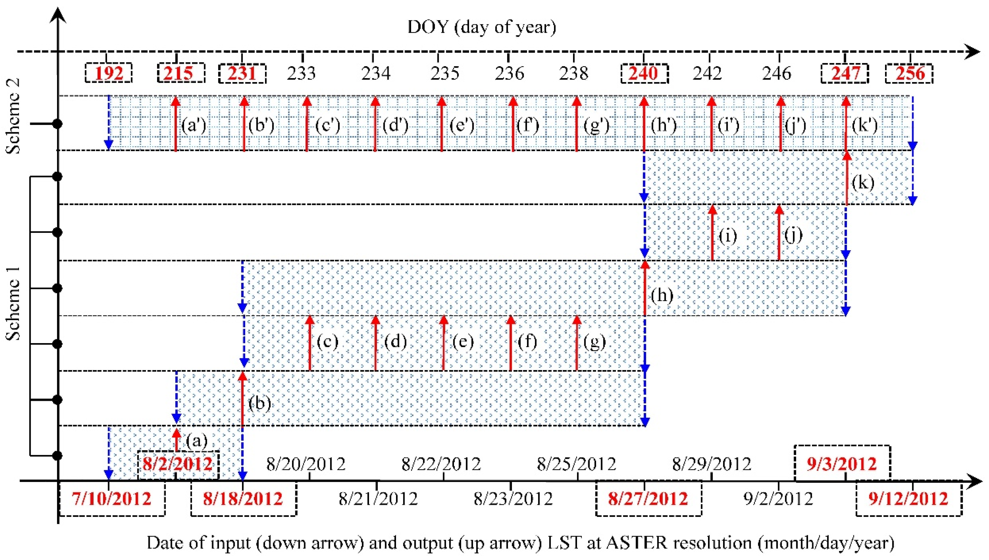
To validate the ESTARFM method for downscaling satellite-retrieved LST data, this study used data from MODIS and ASTER sensors onboard NASA’s TERRA satellite. ASTER was designed to collect data for geological and environmental applications and to provide three spectral bands in the visible near-infrared (VNIR, 0.5–0.9 μm), six bands in the shortwave infrared (SWIR, 1.6–2.5 μm), and five bands in the thermal infrared (TIR, 8–12 μm) regions, with 15-, 30-, and 90-m ground resolutions, respectively [16]. In this study, six ASTER images were acquired from July to September 2012. Table 1 presents a list of all dates and the overpass times of the ASTER data. The land surface temperature and emissivities were derived from the ASTER data using the temperature emissivity separation (TES) algorithm [47], combined with the Water Vapor Scaling (WVS) atmospheric correction method [7,50] which can decrease the uncertainty of the TES algorithm by the parameterization of the sensor view angle and total column water vapor [12,51]. Since the ASTER LST products were generated and evaluated by Wang et al. (2015) [7], here, we just used the LST products without discussing the details of the retrieval method. For a more detailed description of the ASTER LST products, please refer to Wang et al. (2015) [7].
Table 1. A list of dates and statistics results of the ASTER and MODIS LSTs.
CaseDate (Day/Month/Year)Maximum LST (K)Minimum LST (K)Mean LST (K)STD (K)
MODISASTERMODISASTERMODISASTERMODISASTER
110 July 2012323.36325.76301.76299.61309.36310.676.598.02
22 August 2012323.80327.63302.96301.50310.47311.926.678.05
318 August 2012311.72314.32298.82297.34303.43304.293.664.57
427 August 2012320.98323.99301.44299.27308.76309.876.367.63
53 September 2012312.92316.37296.82295.08302.76303.365.196.25
612 September 2012312.38315.28293.97291.95300.93301.455.80 6.95
MODIS is a multispectral imager onboard the Terra and Aqua satellites of NASA’s EOS, and it provides daytime and nighttime imaging capability of any point on the Earth’s surface every 1–2 days, with a spatial resolution of ~1 km at nadir and 5 km at higher off-nadir viewing angles at the scan edge [14]. The LST is retrieved with the new refined generalized split window (GSW) or the day/night LST algorithms, which are view-angle dependent [1,52,53]. Because both ASTER and MODIS are onboard the same satellite platform, observations are made at the same height and coincident nadirs.
Thirteen cloud-free MODIS datasets covering the study area were acquired from July to September 2012 (Figure 2). Each MODIS dataset, including MOD03_L1A, MOD07_L2, MOD09GQ, and MOD11_L2 datasets, was collected from the Land Processes Distributed Active Archive Center (LP DAAC) of the U.S. Geological Survey (USGS). The MOD03_L1A geolocation product contains geodetic coordinates, ground elevation, and satellite zenith and azimuth angles for each MODIS 1-km pixel, which were used in visual interpretations to assist with the accurate coregistration between the MODIS LST and ASTER LST data. The LST products from MOD11_L2 are produced daily at 5-min increments using the generalized split-window algorithm [1,14]. In this study, the acquired ASTER images were first coarsely registered to the MODIS images using the geolocation data provided with the images. Then, the ASTER images were refined by adjusting the integer cross-track and in-track offsets between the MODIS and ASTER images using the area cross-correlation approach [34]. Finally, both the ASTER and MODIS data were registered to the same coordinate system and resampled at the same spatial resolution (90 m). The land cover map in the HiWATER-MUSOEXE experimental area was acquired from the 30-m resolution global land cover (GLC) dataset, GlobeLand30, which includes more than seven land cover types (cultivated land, artificial surfaces, bare land, water bodies, wetland, shrub lands, and forests) [54]. GlobeLand30 datasets were used to classify the land cover into three types in considering the characteristics of land surface coverage in the study area.
Figure 2. Two schemes for estimation of LST at ASTER resolution by ESTARFM. Scheme 1 was a segment-based prediction made by taking turns of each two adjacent temporal data. Scheme 2 was only using first and last temporal data for the direct estimation.
Remotesensing 08 00075 g002

3. Methodology

3.1. Theoretical Basis of the ESTARFM

The ESTARFM algorithm described by Zhu et al. (2010) [20] was applied in the current study, which is described by a linear model in Equation (2) below. The algorithm is based on the assumption that both ASTER and MODIS imagery observe the same reflectance and LST, biased by a constant error. This error is caused by the characteristics of a pixel, and is systematic over short temporal intervals. Therefore, this error can be calculated for each pixel in the image if a base ASTER-MODIS synchronization acquired image pair is available. These errors can then be applied to the MODIS imagery of a prediction date to obtain a corresponding ASTER-like prediction image.
Here, the predicted fine-resolution ASTER-like LST is directly calculated from two pairs of fine- and coarse-resolution images at ta and tc, and the coarse resolution image at tb is only used to calculate the temporal weight at ta and tc.
F b ( x w / 2 , y w / 2 , t b , L S T ) =     [ T a b × F ( x w / 2 , y w / 2 , t a , L S T ) + T c b × F ( x w / 2 , y w / 2 , t c , L S T ) ]                             + i = 1 N W i × H i × [ T a b × ( C ( x i , y i , t b , L S T ) C ( x i , y i , t a , L S T ) ) + T c b × ( C ( x i , y i , t b , L S T ) C ( x i , y i , t c , L S T ) )    ] ​​​​​​​​
T k b = 1 / | i = 1 w j = 1 w C ( x i , y j , t k ) i = 1 w j = 1 w C ( x i , y j , t b ) | k = a , c ( 1 / | i = 1 w j = 1 w C ( x i , y j , t k ) i = 1 w j = 1 w C ( x i , y j , t b ) | ) , ( k = a , c )
where F b is the final predicted fine-resolution LST at the prediction time tb; F and C denote the fine-resolution reflectance and coarse resolution LST, respectively; ta and tc denote the acquisition date for one pair of fine-resolution and coarse-resolution images, respectively; w is the search window size; N is the number of similar pixels including the central “prediction” pixel within the search window; (xi, yi) is the location of the ith similar pixel; Wi is the weight of ith similar pixel; Hi is the conversion coefficient of the ith similar pixel; and T a b and T c b denote the temporal weight at ta and tc as Equation (3), respectively, which can be calculated according to the change in magnitude detected by the resampled coarse-resolution LST between the time (ta or tc) and prediction time tb.
In order to get high spatial-temporal LST from ASTER and MODIS data based on Equation (2), the implementation of ESTARFM consists of three steps. Firstly, a moving window is applied to the ASTER imagery to identify similar neighboring pixels. Secondly, a weight is assigned to each similar neighbor based on: (a) the differences between surface reflectances of ASTER-MODIS image pair and between LSTs of ASTER-MODIS image pair; (b) the temporal difference of the pixel’s value in both MODIS images; and (c) the spatial Euclidean distance between the neighbor and the central pixel. The final step consists of calculating the surface LST of the central pixel. For a more detailed description of the ESTARFM algorithm, please refer to Gao et al. (2006) [18] and Zhu et al. (2010) [20].

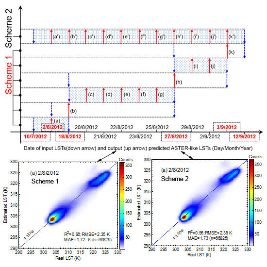
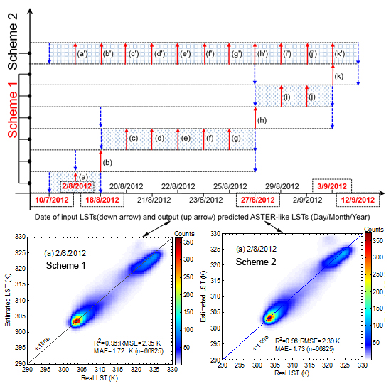
3.2. Evaluation Schemes for Prediction of ASTER-Like LST

In this study, six temporal ASTER LST products already acquired also differed with respect to time intervals. The shortest interval was six days (27 August 2012–3 September 2012), and the longest was 22 days (10 July 2012–2 August 2012). Hence, two schemes for the estimation of 90-m LST were designed (Figure 2). Scheme 1 was a segment-based prediction made using ASTER data acquired on different dates (Figure 2). That is that the two adjacent temporal ASTER/MODIS data were used to estimate the 90-m LST on intermediate dates. In Scheme 1, the ASTER LST products of different dates were input successively to estimate the 90-m LST with ESTARFM. Because the ASTER LST products had different time intervals, the different temporal ASTER LST data were used as the input with different frequencies; the smallest frequency was 1 (10 July, 2 August, 12 September 2012) and the largest was 4 (27 August 2012). Finally, the 11 temporal LSTs at a 90-m resolution were estimated successively. In Scheme 2 (Figure 2), the two temporal ASTER/MODIS data, 10 July 2012 and 12 September 2012, were used for the direct estimation of the 11 temporal LSTs at the 90-m resolution.
The 90 m LST estimated by ESTARFM was validated with three experiments. (1) The simulation data of typical ground objects (water surface, vegetation) were chosen for the validation by changing their LST, shape, and size. With reference to the simulation tests conducted by Gao et al. (2006) [18] and Zhu et al. (2010) [20], we tested four cases: varying temperature/reflectance, varying shapes, predicting small objects, and predicting linear objects. In detail, a series of 198 × 198 pixel fine-resolution images were first simulated by assigning each pixel a positive value ranging from 290 to 320 or 0 to 1 to denote the temperature or reflectance of each pixel, respectively. Coarse-resolution images were produced by scaling-up the fine-resolution images (i.e., each cluster of 11 × 11 neighboring pixels in the fine-resolution image was aggregated to create a pixel in a coarse-resolution image). The spatial resolutions of fine- and coarse-resolution simulated images were identical to those of ASTER and MODIS. Specifically, three pairs of fine- and coarse-resolution images acquired on the same date were simulated. Then, the first and last pairs and the coarse-resolution image of the second pair were used to predict the fine-resolution image of the second pair, and the predicted and real images were compared to assess the accuracy of the new algorithm; (2) Using the schemes in Figure 2, the four temporal ASTER LST products (2 August, 18 August, 27 August and 3 September 2012) were chosen for the validation of LST estimated by ESTARFM; (3) The LST estimated by ESTARFM was validated with the LST measurements of the radiometer equipped at the WATERNET stations and AWSs in HiWATER-MUSOEXE. Here, the normalized error index (NEI) is used to express the relative LSTs’ deviation between the ESTARFM estimated LSTs and ground measurements while varying the number of land cover types and the size of search window. It can be described as Equation (4).
N E I = M a x ( σ ) σ M a x ( σ ) M i n ( σ ) , σ = L S T G r o u n d L S T E S T A R F M
where σ is the LST predicted errors by the ESTARFM comparing to ground measurements, M a x ( σ ) is the maximum of σ , and M i n ( σ ) is the minimum of σ .

4. Results

4.1. Evaluation of ESTARFM by Simulation

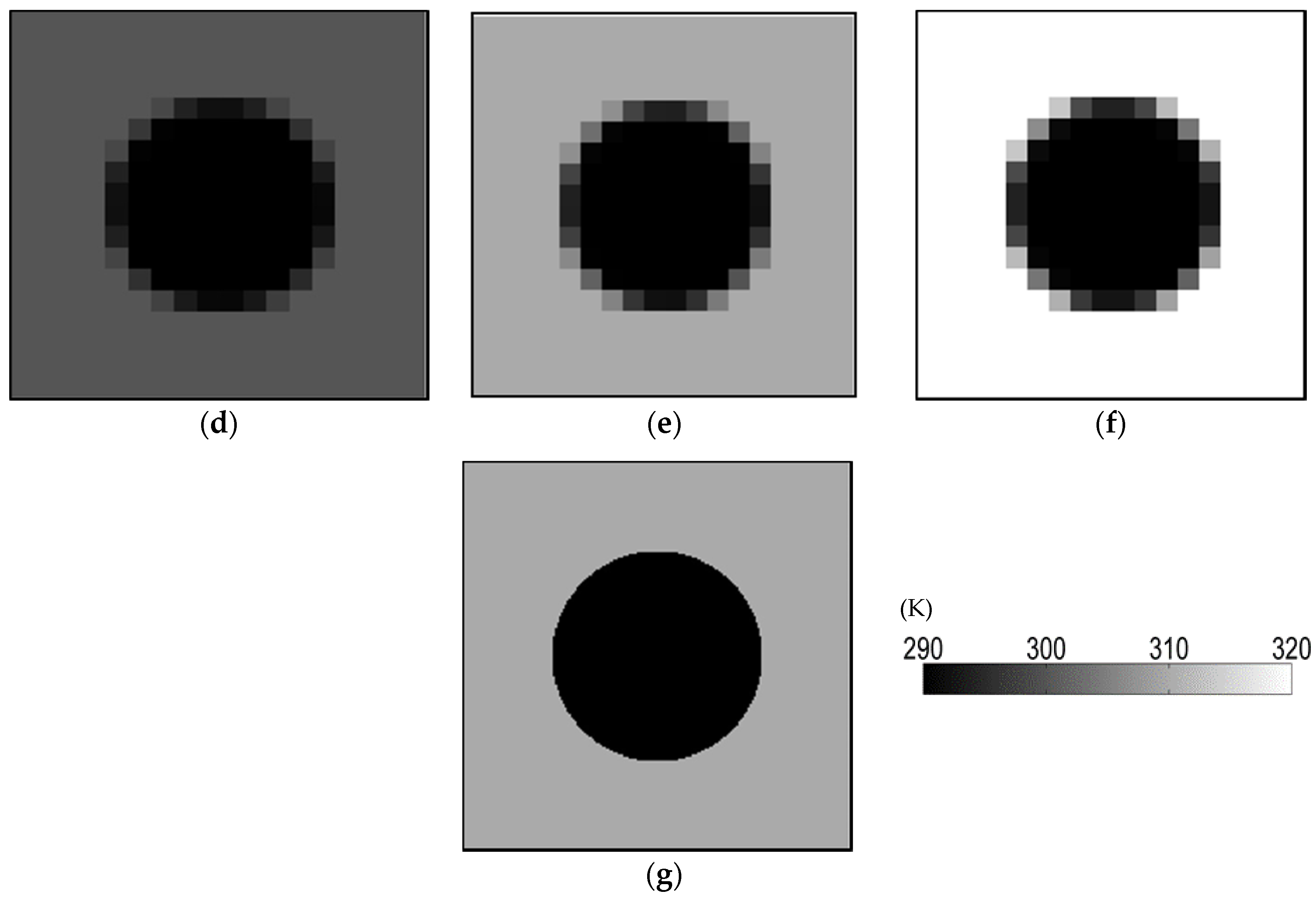
4.1.1. Test with Varying Temperature

The ESTARFM algorithm was tested with simulated temperature and reflectance data to help understand its effectiveness and limitations. In this simple case, there were only two objects (e.g., water and vegetation) (Figure 3). The shapes of water and vegetation were fixed, and we assumed that the water body (circle) had a constant surface reflectance of 0.05 and a constant temperature of 290 K over the observing period, whereas the vegetation reflectance was set as 0.1, 0.2, and 0.4, and the corresponding temperature was set as 300 K (Figure 3a), 310 K (Figure 3b), and 320 K (Figure 3c). The MODIS-like 990-m spatial resolution temperature images (Figure 3d–f) were aggregated from the ASTER-like 90-m spatial resolution images (Figure 3a–c). Using the ESTARFM algorithm and data from Figure 3a,c–f, we estimated the fine-resolution temperature image (Figure 3b). When the surrounding spatial information of fine-resolution data was used, a nearly exact match (Figure 3g) could be retrieved at a finer resolution in this simple case. Zhu et al. (2010) [20] conducted a similar study for downscaling land surface reflectance data from MODIS resolution to Landsat ETM+ resolution using an enhanced spatial and temporal adaptive reflectance fusion model. This example reveals the significance of additional fine resolution spatial information from multisource remote sensing data to downscaling LST.
Figure 3. Simulation of temporal changes in temperature for water (inside circle) and vegetation (outside circle). (ac) were fine resolution images for three temporal; (df) were coarse-resolution images aggregated from fine resolution images (ac); Image in (g) was estimated with ESTARFM, for comparison with image (b).
Remotesensing 08 00075 g003aRemotesensing 08 00075 g003b

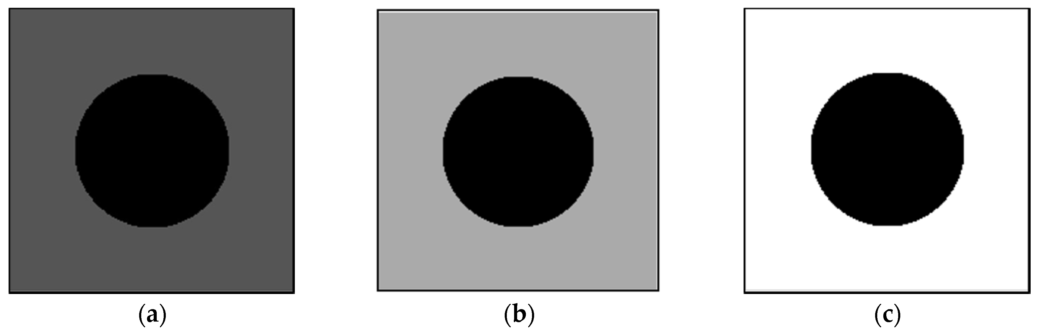
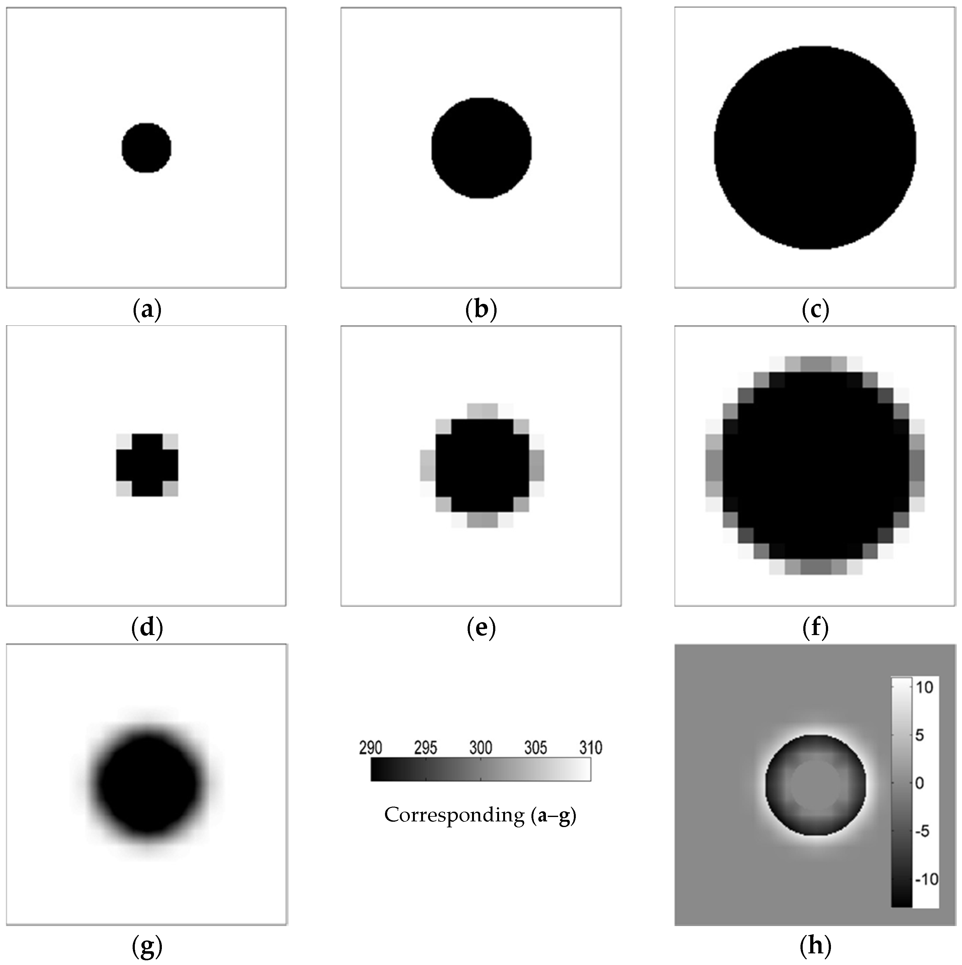
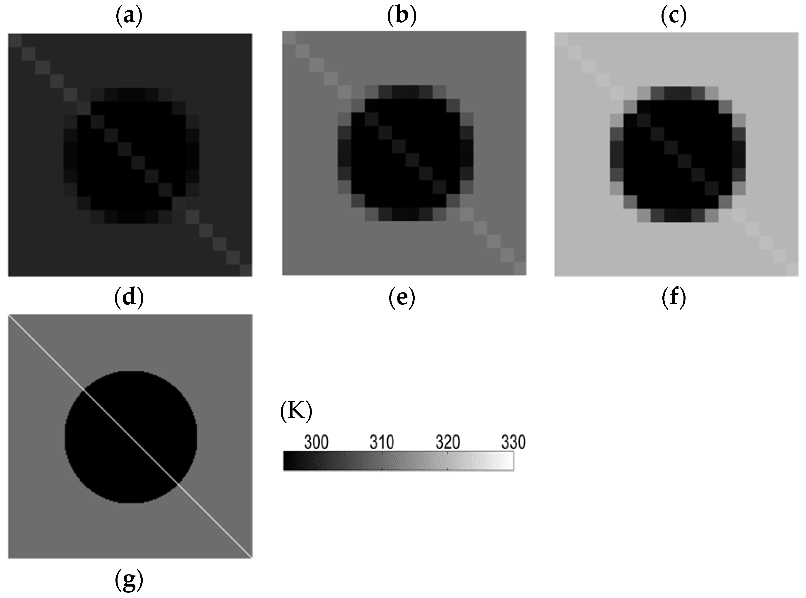
4.1.2. Test with Changing Shapes, Small Objects, and Linear Objects

(A) Changing Shapes

Land cover may change over a growing season, not just in terms of overall temperature and reflectance, but also in terms of shape and size. To better understand the ESTARFM algorithm’s performance, we assumed that the surface reflectance was constant with time for the two land-cover types; the background reflectance was 0.2; the background temperature was 310 K; the circular object reflectance was 0.05; and the circular object temperature was 290 K. The radius of the circular object was set as 500 m (Figure 4a,d), 1000 m (Figure 4b,e), and 2000 m (Figure 4c,f). Figure 4a–c shows the simulated ASTER-like 90-m temperature images. The MODIS-like 990-m resolution data (Figure 4d–f) were aggregated from the ASTER-resolution views. Figure 4g is the image predicted from fine-resolution data (Figure 4a,c) and coarse-resolution data (Figure 4d–f), including additional spatial information. Figure 4h is the absolute difference between true (Figure 4b) and predicted data (Figure 4g). It shows that the differences were greatest along the annular region (Figure 4h), ranging from the inner ring in Figure 4a to the outer ring in Figure 4b, where the radius represents the estimated temperature and the corresponding prediction errors increased compared with the true values (Figure 4b). However, the image also shows the opposite result, ranging from inner ring in Figure 4b to the outer ring in Figure 4c. According to the ESTARFM algorithm, Figure 4g was calculated by weighting the first prediction from Figure 4a to Figure 4b, and the second prediction from Figure 4c to Figure 4b. Overlapping and non-overlapping regions were included in the total area during the prediction process. There were no temperature changes within overlapping regions between Figure 4a,b or between Figure 4b,c, respectively. Therefore, there were no prediction errors due to overlapping regions. However, there were large errors within non-overlapping regions, which were mainly caused by mixed pixels. For instance, in the annular region ranging from the inner ring in Figure 4a to the outer ring in Figure 4b, the value of mixed pixels in Figure 4e was greater than the true values in Figure 4b, resulting in overestimated temperature and a maximum error along the border of the circular region (Figure 4h). In contrast, temperature was underestimated within non-overlapping regions between Figure 4b,c.
Figure 4. Simulation of an object with changing shape. (ac) were fine resolution images for three temporal; (df) were coarse-resolution images aggregated from fine resolution images (ac); Image in (g) was estimated with ESTARFM, for comparison with image (b); Image in (h) was difference between (b,g).
Remotesensing 08 00075 g004

(B) Small Objects

Similar to the previous simulation in Figure 3, we assumed that a water body (circle) had a constant surface temperature and reflectance with a radius of 990 m (11 fine-resolution pixels). The background vegetation (outside the circle) reflectance was set as 0.1, 0.2, and 0.4, and the corresponding temperature was set as 300 K, 310 K, and 320 K for three different periods (Figure 5). It is obvious that the ESTARFM algorithm can predict the shape of the small circular object. Moreover, the predicted temperature (Figure 5g) of the small circular object from the ESTARFM is close to that in Figure 5b.
Figure 5. Simulation test on a small object. (ac) were fine resolution images for three temporal; (df) were coarse-resolution images aggregated from fine resolution images (ac); Image in (g) was estimated with ESTARFM, for comparison with image (b).
Remotesensing 08 00075 g005

(C) Linear Objects

Linear objects such as roads and small rivers are normally visible in fine-resolution ASTER imagery but are not obvious in coarse-resolution MODIS imagery. For the linear object example, the simulated fine-resolution images contained three objects: the background with temperature was set as 300 K (Figure 6a), 310 K (Figure 6b), and 320 K (Figure 6c) and the corresponding reflectance was set as 0.1, 0.2, and 0.4. The simulated water body (circle) had a constant reflectance of 0.05 and temperature of 295 K. The simulated road (over background) and bridge (over water) had a constant reflectance of 0.5 and temperature of 330 K. The MODIS-like data in Figure 6d–f were aggregated from the ASTER-like data. Roads (over background) are still visible in Figure 6d,e but not in Figure 6f owing to the smaller contrast between roads and the background in Figure 6c. Figure 6g is a predicted version of Figure 6b using fine-resolution (Figure 6a,c) and coarse resolution (Figure 6d–f) images with an additional neighboring pixel spatial-information option turned on. The result shows that ESTARFM can exactly predict the shape of the linear object (Figure 6g).
Figure 6. Simulation test on a linear object. (ac) were fine resolution images for three temporal; (df) were coarse-resolution images aggregated from fine resolution images (ac); Image in (g) was estimated with ESTARFM, for comparison with image (b).
Remotesensing 08 00075 g006aRemotesensing 08 00075 g006b

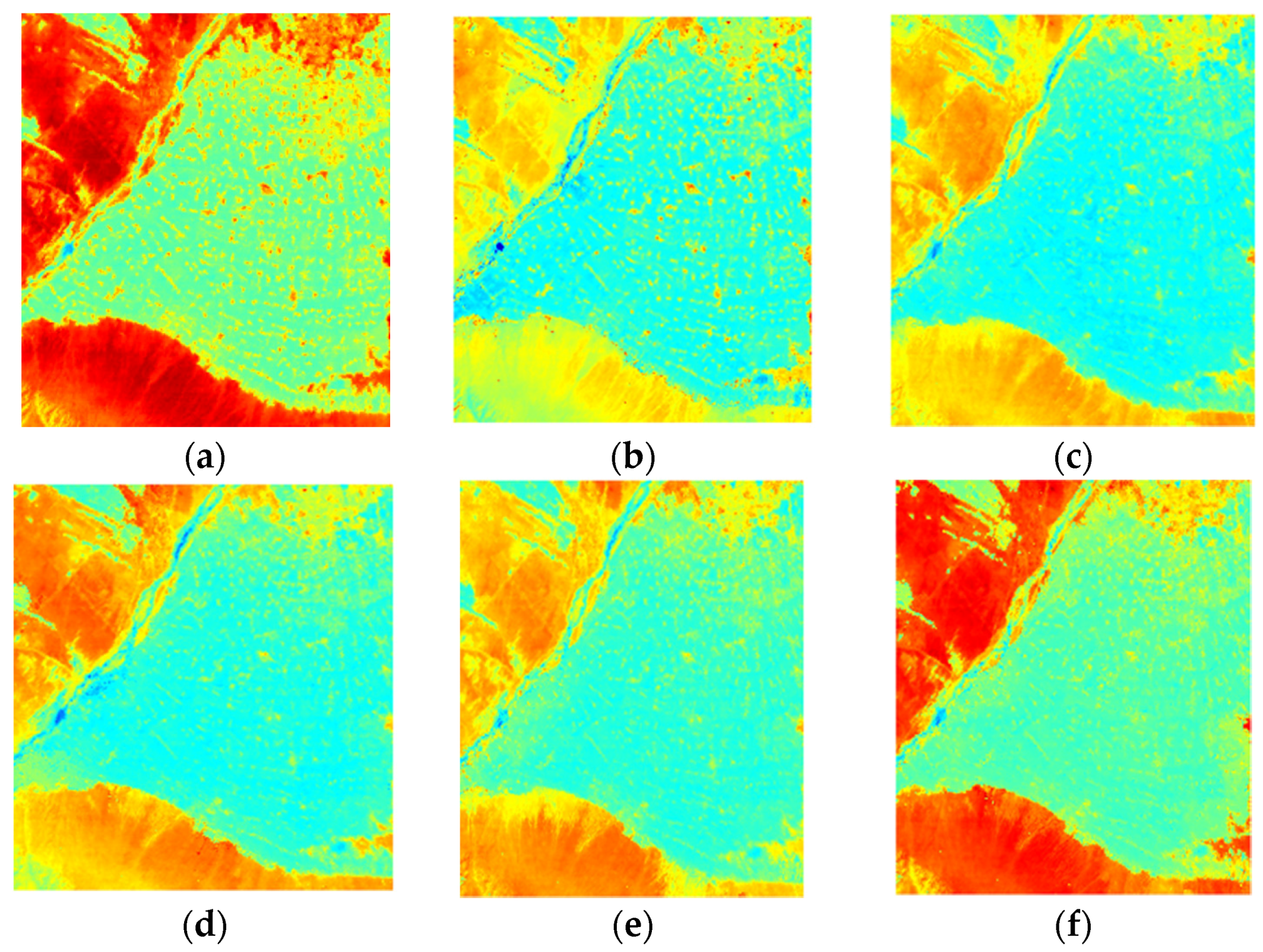
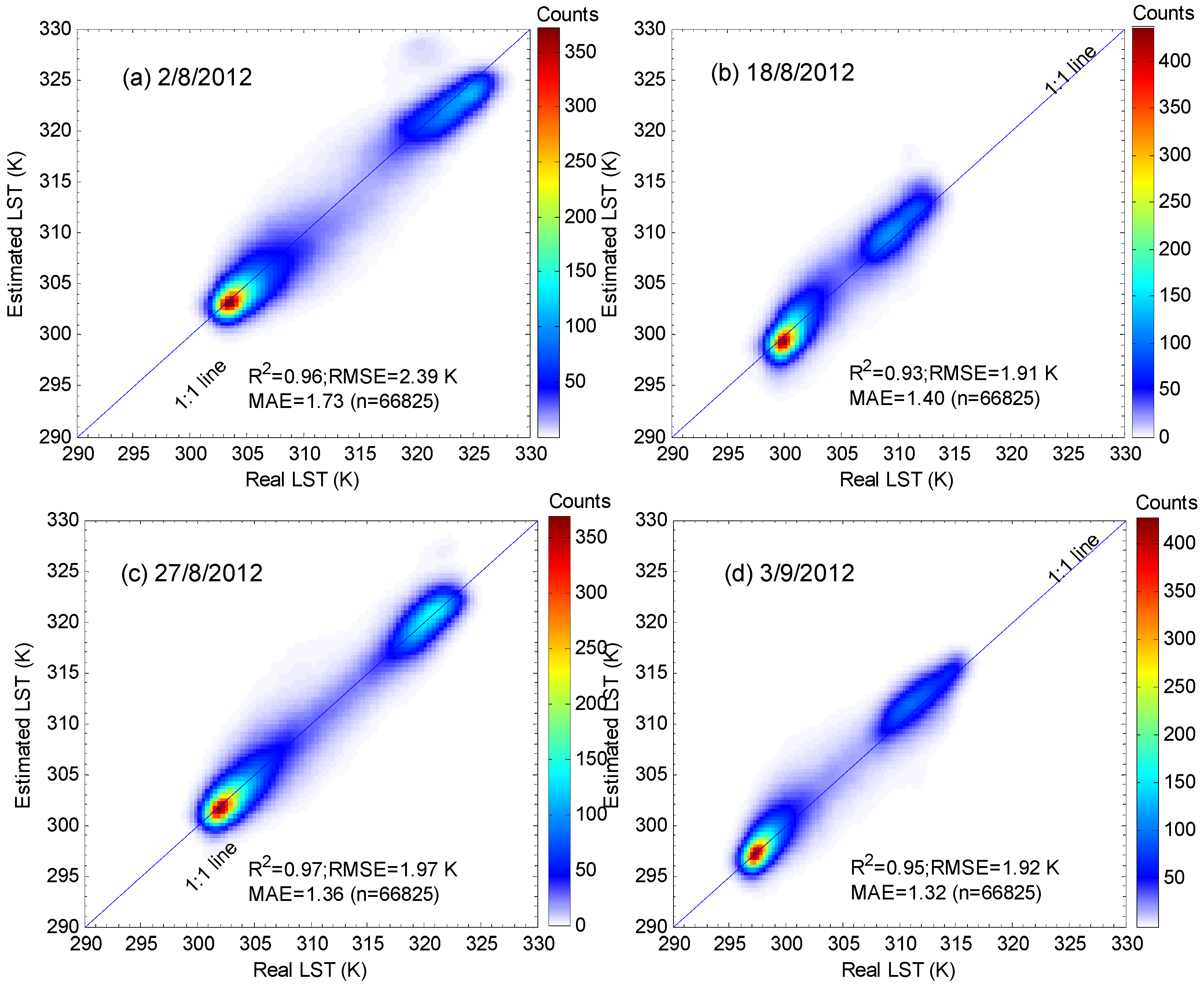
4.2. Tests with ASTER LST Products
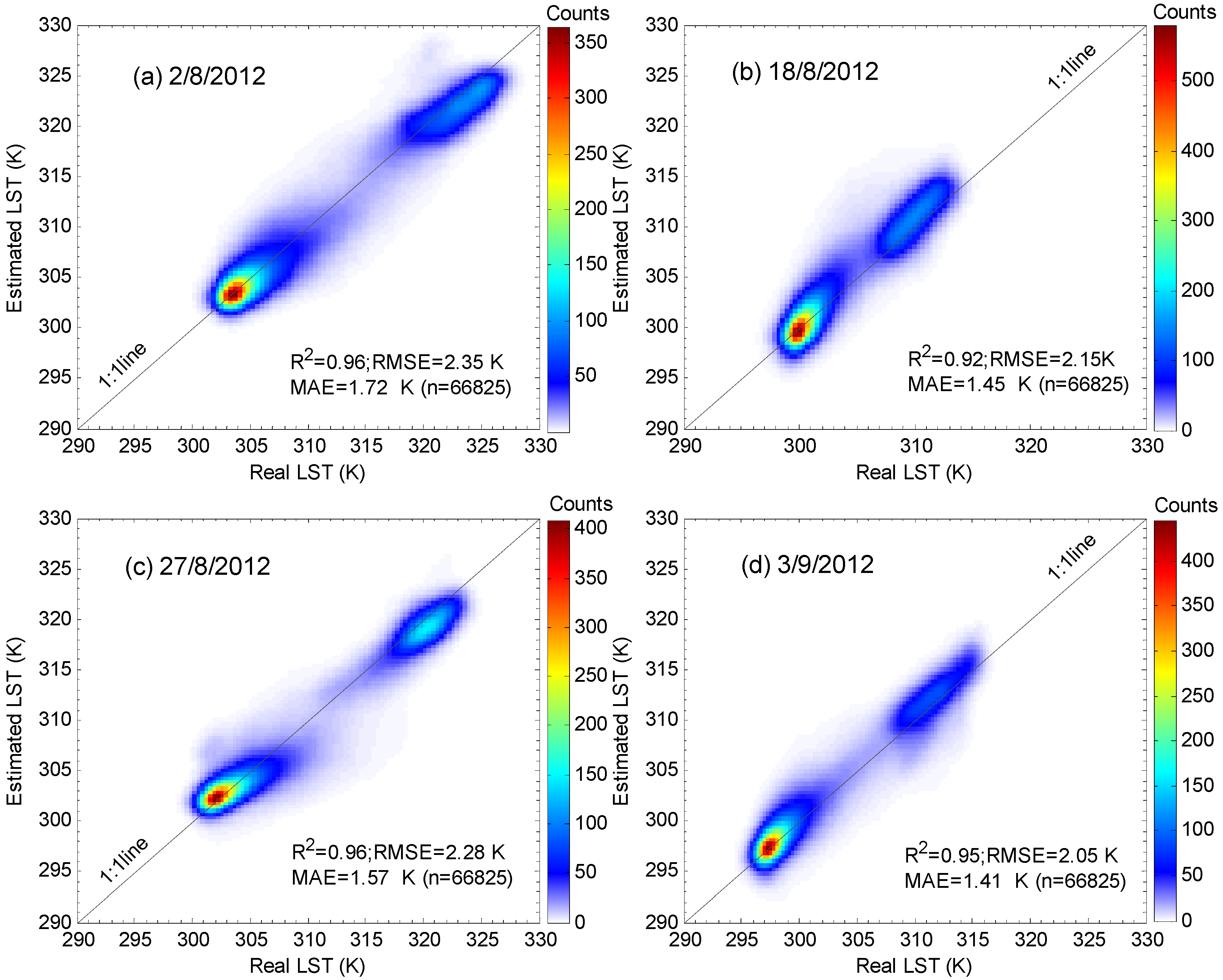
According to the schemes in Figure 2, two groups of ASTER-like 90-m LSTs were estimated with ESTARFM (Figure 7 and Figure 8). In general, the 11 temporal LST products at the 90-m resolution estimated by the two schemes were consistent.
Figure 7. Estimated LST with ASTER resolution using ESTARFM according to Scheme 1. (a) 2 August 2012; (b) 18 August 2012; (c) 20 August 2012; (d) 21 August 2012; (e) 22 August 2012; (f) 23 August 2012; (g) 25 August 2012; (h) 27 August 2012; (i) 29 August 2012; (j) 2 September 2012; (k) 3 September 2012.
Remotesensing 08 00075 g007aRemotesensing 08 00075 g007b
Figure 8. Estimated LST with ASTER resolution using ESTARFM according to Scheme 2. (a) 2 August 2012; (b) 18 August 2012; (c) 20 August 2012; (d) 21 August 2012; (e) 22 August 2012; (f) 23 August 2012; (g) 25 August 2012; (h) 27 August 2012; (i) 29 August 2012; (j) 2 September 2012; (k) 3 September 2012.
Remotesensing 08 00075 g008aRemotesensing 08 00075 g008b
ASTER LST products with a 90-m spatial resolution were used as real values for the validation of ASTER-like 90-m LSTs estimated by ESTARFM. The prediction accuracy for all pixels of ESTARFM was evaluated with the correlation coefficient (R2), root-mean-square error (RMSE), and mean absolute error (MAE). The number of land cover types was set as three: vegetated, non-vegetated, and water. The size of the search window was set as 22 ASTER pixels at 90-m or 2 MODIS pixels at 990-m spatial resolution. The ASTER data from the first date (10 July 2012) and last date (12 September 2012) was used as input data for ESTARFM. Thus, it was impossible to estimate the ASTER-like 90-m LSTs of these two dates. The ASTER LST products were employed to validate the LST estimates of the four dates (2 August, 18 August, 27 August and 3 September 2012). Figure 9 and Figure 10 display the scatter plots between the predicted ASTER-like and real ASTER LST products based on Schemes 1 and 2 in Figure 2, respectively. The data points fell close to the 1:1 diagonal line in each panel, indicating that the predictions all agreed well with the observations. To quantify the prediction accuracy, the R2, RMSE, and MAE for each land cover type and the total area were calculated. Table 2 shows the computation results for the two schemes (Figure 2). Overall, the values of R2, MAE, and RMSE between the ASTER-like and observed LSTs for the average of the three land cover types, were quite close with the two schemes. The R2 values of the two schemes were all greater than 0.92. The MAE ranged from 1.32 K to 1.73 K and the RMSE ranged from 1.92 K to 2.39 K for the two schemes. The possible reason was that, the short-term, transient land cover changes over croplands were little and can be ignored during the maize growing period from July to September, 2012 although the selected images also reflected the phenological changes.
The accuracies of LST estimates made with Schemes 1 and 2 were calculated for the three individual land cover types. In general, the accuracies of LSTs estimated by the two schemes were consistent for the same land cover type. There was some variation in the prediction accuracy for different land cover types. The order of land cover types with respect to their RMSE or MAE values was non-vegetated > vegetated > water. The following is a detailed analysis of the estimations made using Scheme 2. The correlation coefficient between the predicted and observed LSTs was the highest in non-vegetated areas, and the R2 values of all four dates were larger than 0.82. The order of land cover types with respect to their respective R2 values was non-vegetated > vegetated > water. The RMSEs for water were the smallest (all lower than 0.22 K), whereas the RMSEs for non-vegetated areas were the highest (all higher than 1.5 K). The predicted LSTs had close RMSEs for the three land cover types at different dates. The order of the land cover types with respect to the average RMSE of the four dates was non-vegetated > vegetated > water. The MAE for water was the smallest on all four dates, with a value close to 0.02 K. The MAE of non-vegetated areas was the largest, with a value of 1.0 K (2 August 2012). The order of land cover types based on the average MAE for the four dates was the same as that based on RMSE (i.e., non-vegetated > vegetated > water). The correlation coefficient between the predicted and observed LSTs of water in the four dates was low. However, the RMSE and MAE between the predicted and observed LSTs of water were five-times lower than that of the other two land cover types.
Figure 9. Scatter density plots between the observed product and estimated LSTs with Scheme 1 on 8 August 2012 (a); 18 August 2012 (b); 27 August 2012 (c); and 3 September 2012 (d).
Remotesensing 08 00075 g009
Figure 10. Scatter density plots between the observed product and estimated LSTs with Scheme 2 on 2 August 2012 (a); 18 August 2012 (b); 27 August 2012 (c); and 3 September 2012 (d).
Remotesensing 08 00075 g010
Table 2. The accuracy of estimated LST for overall and individual land cover types by two schemes (K).
SchemeDate (D/M/Y)Correlation Coefficient (R2)Root Mean Square Error (RMSE)Mean Absolute Error (MAE)
OverallVegetationNon-VegetationWaterOverallVegetationNon-VegetationWaterOverallVegetationNon-VegetationWater
12 August 20120.960.680.880.552.351.311.890.221.720.681.030.02
18 August 20120.920.740.780.682.151.001.860.231.450.490.940.02
27 August 20120.960.620.910.632.281.261.860.201.570.600.950.02
3 September 20120.950.640.870.742.051.091.690.141.410.520.880.01
22 August 20120.960.680.880.552.391.361.900.221.730.711.000.02
18 August 20120.930.640.820.641.911.071.550.181.400.570.810.02
27 August 20120.970.740.920.601.971.211.500.201.360.610.730.02
3 September 20120.950.650.890.701.921.031.570.151.320.520.790.02
The spatial homogeneity analysis of each land cover type with a 90-m spatial resolution in the study area showed that the main ground object in the non-vegetated area was Gobi desert. This homogeneity of the Gobi desert at different dates did not significantly vary. Therefore, the accuracy of the 90-m LST predictions with ESTARFM was high. The vegetated area was mainly cultivated with crops such as spring wheat and summer maize. During the period from July to September, the vegetation coverage changed with the growth, maturity, and harvest of the crops. Vegetation coverage had a strong negative correlation with LST [29,45], which had a major influence on LST homogeneity. As a result, the influence of land surface homogeneity would cause an uncertainty for calculation of the weight coefficient using ESTARFM. The waters in the Heihe River Basin represented the main water type in the study area. The water amount of the rivers decreased from July to September. Most of the tributaries dried up, causing significant variation in the area through which the rivers flows at different dates. The water body coverage is only 0.69%, and most rivers and Gobi desert in the study area formed mixed pixels. Consequently, the uncertainty of LST estimated by ESTARFM increased.
As indicated by accuracy comparisons between Schemes 1 and 2, when there was no obvious change in land cover type and only a seasonal change in vegetation coverage, remote sensing data from only two dates were needed for LST predictions over a little bit longer time period (10 July 2012–12 September 2012). High-accurate LST predictions can be achieved at any intermediate times. These results suggest that ESTARFM would have a high reliability when predicting long time series of LSTs.

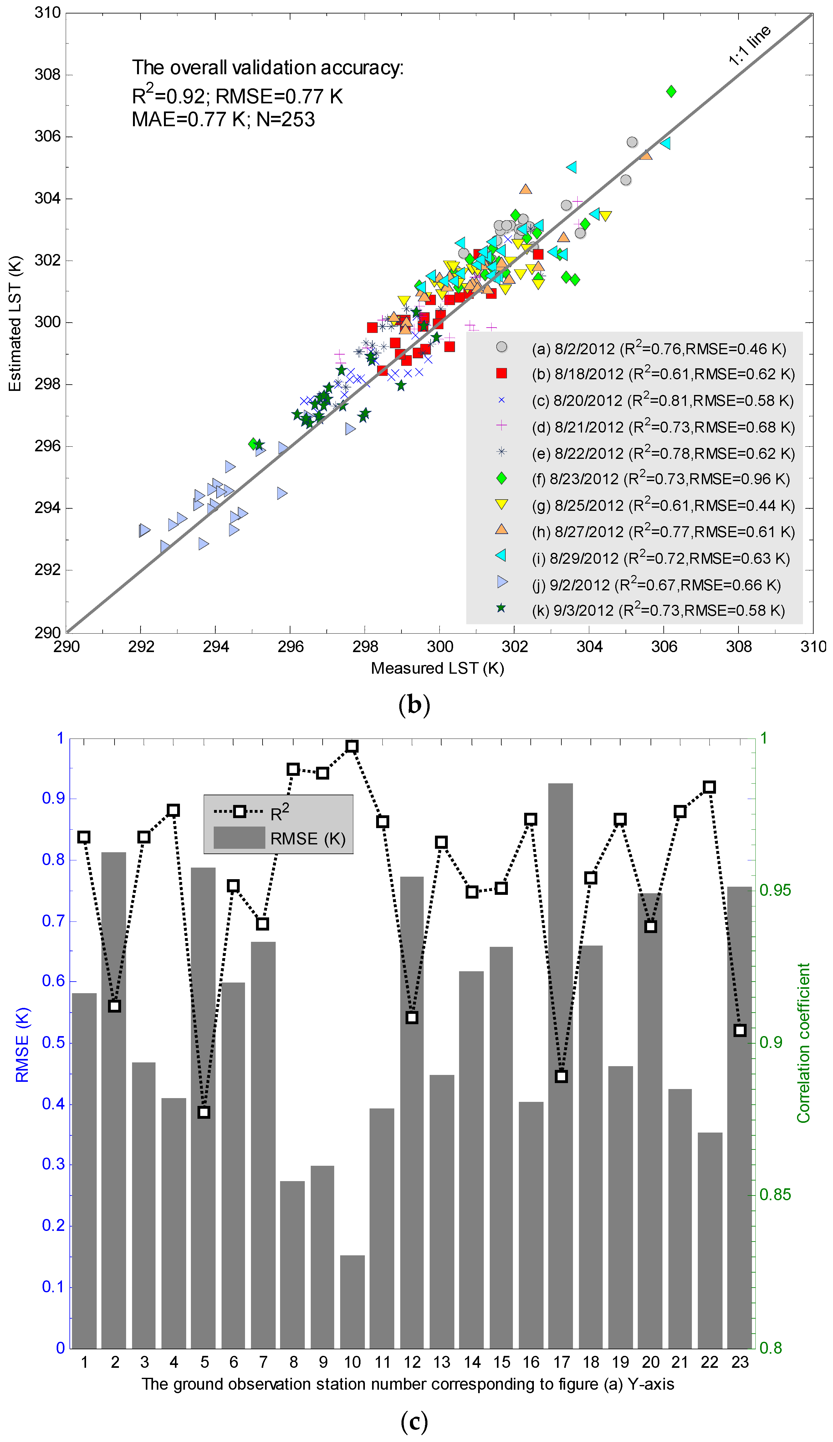
4.3. Tests with Ground Measurements

The LST measurements taken with the SI-111 radiometer at 12 AWSs and 27 WATERNET stations in the HiWATER-MUSOEXE experiment were used to validate the LST predictions. Wan et al. (2008) suggested that the uncertainty of the LST at ideal stations for a homogeneity validation should be less than 1 K. The latitude and longitude of 39 (12 + 27) ground observation sites were used to extract the LSTs of nine pixels within the range of 3 × 3 pixels from 11 predicted scenes of ASTER LST (Figure 8). The STD (standard deviation) of the LSTs of nine pixels was calculated. The average STD of the all dates for each satellite image at each observation station was calculated. Observation sites with an average STD lower than 1 K were chosen as sites for the final ground validation. A total of 23 observation sites were screened based on the above conditions, including nine AWSs and 14 WATERNET stations (Figure 11).
Figure 11. The average STD of LSTs at all AWS and WATERNET stations.
Remotesensing 08 00075 g011
The LST measurements made on different dates at 23 observation sites were chosen to validate the estimated LSTs, as shown in Figure 12. The error distribution of LSTs predicted by ESTARFM was [−1.5, 2.4] K, as shown in Figure 12a. Figure 12b shows the overall validation accuracy (R2 = 0.92, RMSE = 0.77 K). There was a certain amount of variation in the validation accuracy on different dates. The LST estimates on different dates were validated by the LST measurements. That is that the LST at each observation station was used to perform a validation analysis of time series (Figure 12c). As shown in Figure 12c, the R2 value was generally higher than 0.9 (except for the station WATERNET 42). This indicated that the variation trend of LSTs predicted by ESTARFM was consistent with that of measured LSTs at each observation station. The RMSE of LSTs estimated by ESTARFM at each observation station was smaller than 1 K. This was consistent with the condition for the selection of LST observation sites (i.e., STD < 1 K).
Figure 12. Error image and correlation analysis plot for LST ground validation. (a) Image of errors between estimated and measured LSTs for each date (horizontal axis) and stations (vertical axis); (b) Scatter plot of measured and estimated LSTs on 11 dates (2 August–3 September] and overall accuracy; (c) Correlation coefficient and RMSE between estimated and measured LSTs for each ground observation including all dates.
Remotesensing 08 00075 g012aRemotesensing 08 00075 g012b

5. Discussion

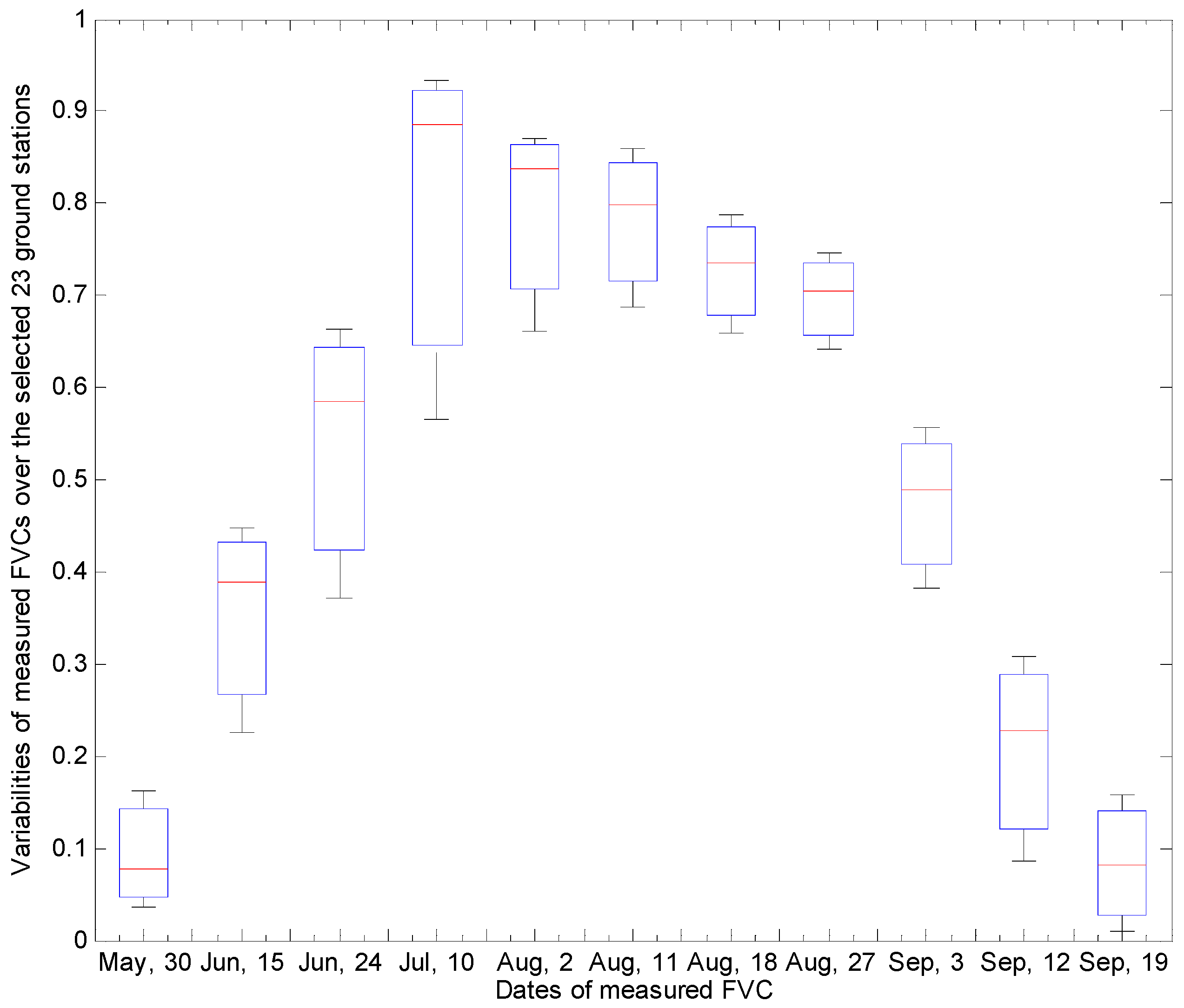
5.1. Uncertainty of LST Spatial Variance

In MODIS and ASTER, the LST is retrieved with the generalized split-window algorithm [1,14] and the temperature emissivity separation (TES) algorithm combined with the WVS method [47,50,51], respectively. Due to the large differences in the retrieval algorithms, there was a certain variation retrieved in LST [12]. In this study, although the mean LST and STD of ASTER and MODIS LSTs were coordinated, the LST variation range of ASTER was greater than MODIS. The variation range for MODIS LST was within the ASTER LST range for each pair of acquired MODIS and ASTER data at the same date (Table 1). To some extent, these deviations were caused by land surface heterogeneity. Therefore, it was only necessary to choose an area with homogeneous land cover types in ESTARFM to calculate the conversion coefficients (Hi) of MODIS and ASTER LSTs. The errors arising from the differences in the retrieval algorithms could be reduced.
The non-vegetated area was mainly composed of extensive Gobi desert, which varied very little over the entire research period. Therefore, ESTARFM had a higher prediction accuracy for this area. Crops covered a majority of the vegetated area, and the coverage decreased with varying extents over the entire research period (10 July–12 September 2012) (Figure 13). It can be seen from Figure 13 that the vegetation coverage (i.e., FVC) of 23 observation sites declined by [0.1, 0.4]. As the extent of the reduction in coverage differed at different sites, the heterogeneity of land surfaces increased, which affected the prediction accuracy of ESTARFM. The main water types in the study area were linear rivers and inconsistently distributed planar water bodies. The surface water in the study area was mainly comprised of snowmelt from high mountains. Under the influence of snowmelt, the flow area and position of rivers varied. The variation in the morphology of ground objects also affected the prediction accuracy of ESTARFM, as already shown by the validation using the simulation data (Figure 4).
Figure 13. Variation range of 23 selected stations’ FVC from 30 May to 19 September 2012.
Remotesensing 08 00075 g013
On the basis of simulation testing with changing shapes, small objects, and linear objects, it can be concluded that the ESTARFM approach cannot accurately predict objects whose shape changes over time, and will thus blur the changing boundary. It also cannot accurately predict short-term disturbances and changes that are not recorded in any of the bracketed fine-resolution images. The best way to solve this problem is to identify spatial and temporal changes in the landscape with a high level of detail and to select the last MODIS and ASTER image pair for predictions [19].

5.2. Uncertainty of the ESTARFM Input Parameters

There is a need to pay special attention to the two input parameters, the number of land cover types and the size of the search window for the ESTARFM. In the tests with ASTER LST products, we directly gave constant values of the two parameters (i.e., the number of land cover types was set as 3 and the size of the search window was set as 22). Although the total number of land cover types in the study area was unchanged from July to August 2012, and the three land cover types—non-vegetation, vegetation and water area—remained the same during the period. However, a swap of a part of the pixels among the three land cover types would take place in different temporal images. Therefore, when applying the ESTARFM algorithm, the number of land cover types would be changed with the position of the window and corresponding temporal image. For example, with the image on 3 September 2012 (Figure 14a), we tested the different number of land cover types and compared the results with ground temperature measurements in HiWATER-MUSOEXE. Figure 14a illustrated different NEI values with varying number of land cover types at each station. When an NEI value was close to zero, the corresponding number of land cover types is optimal.
For finding a similar pixel process in ESTARFM, the size of the moving window played an important role in searching for similar pixels and directly affected their weight distribution. In fact, based on the principle of ESTARFM algorithm, the basis of searching for similar pixels was spectral and temperature similarity. In other words, the degree of land surface heterogeneity determines the size of window, and thus affects results from finding similar pixels. Therefore, the size of window should be appropriately determined when the ESTARFM is applied to other areas. Figure 14b showed that the size of window should be set at 13 and 19 for the images on 2 August and 3 September, respectively. The best way to optimize the size of search window for each temporal image in the next step is suggested to use the ESTARFM method coupled with a ground measurement-based assimilation approach [31].
Figure 14. Impact analyses of the number of land cover types and the size of search window for ESTARFM, (a) NEI with different land cover type; (b) NEI with different size of window.
Remotesensing 08 00075 g014
In this study, the annual temperature cycle (ATC) model [24] was not employed to consider the seasonality variations of land surface temperature. First, an ATC model can approximate the long term seasonal cycles of LST, but it cannot delineate the specific daily weather and surface conditions that may also affect the temporal variation in daily LST, leading to uncertainty in the model. Second, the phase shift parameter of the ATC for each predicted pixel was constant. In fact, the phase shift parameter of the ATC model for different ground objects also differed. The phase shift parameter of the ATC model differed even under different time scales of the ground objects [11]. Furthermore, as the evaluation results of the ESTARFM by simulation mentioned Section 4.1.1, the ESTARFM can estimate object LST with high accuracy without spatial shape change, just temperature variation within season. Therefore, a suitable way to deal with LST prediction for objects with shape changes is using closely temporal MODIS LST to predict ASTER-like LST.

6. Conclusions

In this study, we tested ESTARFM to generate an ASTER-like LST using combined MODIS and ASTER datasets. We successfully examined the implementation and validation procedures of ESTARFM based on six ASTER and 13 MODIS cloud-free observations made from July to September 2012 (Figure 2) over an arid oasis area of Northwest China.
We validated ESTARFM using simulation data. The results indicated that ESTARFM could accurately predict ground objects with temperature variations. The prediction was also accurate for small ground objects and linear ground objects. The ASTER-like 90-m LSTs estimated by the two schemes at 11 succession dates were consistent. This indicated the reliability of ESTARFM for the prediction of long LST time series. The 90-m ASTER LST products were used as real values. The ASTER-like 90-m LSTs estimated by ESTARFM were validated. The overall R2 values of the predicted LSTs on four dates (2 August, 18 August, 27 August, and 3 September 2012) were larger than 0.92. The MAE of the two schemes ranged from 1.32 K to 1.73 K, and the RMSE ranged from 1.92 K to 2.39 K. The order of land type with respect to the corresponding R2, RMSE, and MAE values was non-vegetated > vegetated > water.
A total of 23 observation sites were selected from the HiWATER-MUSOEXE experiment. The LST measurements made by SI-111 radiometers at each observation station were used to validate the ASTER-like LSTs predicted on the 11 dates. The results indicated that the overall accuracy was high (R2 = 0.92, RMSE = 0.77 K). The error distribution of LST predicted by ESTARFM was [−1.5, 1.5] K. Moreover, the predicted LSTs at the same observation station but different dates were also validated. The R2 values were higher than 0.9 (except at the WATERNET42 station). The RMSE of LSTs predicted at each observation station with ESTARFM was less than 1 K.
There are two major limitations as previously reported by Zhu et al. (2010) that should be considered when using the ESTARFM approach to predict LST. First, ESTARFM cannot accurately predict short-term, transient LST changes that are not recorded in any bracketed fine-resolution images, which was proved by changing shapes within the simulation validation in Section 4.1.2. Therefore, combining ESTARFM with STAARCH [19] or STRUM [40] algorithms may be a feasible way to enhance the capability of the new algorithm. Secondly, ESTARFM may be computationally intensive and require at least two pairs of fine- and coarse-resolution images acquired on the same day. More frequent intra-annual images are helpful to bracket all vegetation phenology changes. However, in some cloudy regions, it is difficult to acquire two high-quality input pairs simultaneously. Mismatching between ASTER and MODIS pixels was neglected in this study. The variation in the MODIS pixel footprint, especially for off-nadir viewing, may have caused some errors and needs to be considered.

Acknowledgments

This study was supported by the Natural Science Foundation of China (41271345), the Beijing Natural Science Foundation (4141001), the National High Technology Research and Development Program of China (2013AA102303) and the Special Funds for Technology innovation capacity building sponsored by the Beijing Academy of Agriculture and Forestry Sciences (KJCX20140417). We are grateful to the anonymous reviewers for their valuable comments and recommendations.

Author Contributions

Guijun Yang and Chenhong Sun analysed data and wrote the manuscript; Qihao Weng, Ruiliang Pu, Feng Gao and Chunjiang Zhao gave comments, suggestions to the manuscript, and checked the writing; Hua Li provided data and data acquisition capacity.

Conflicts of Interest

The authors declare no conflict of interest.

References

  1. Wan, Z. New refinements and validation of the MODIS land-surface temperature/emissivity products. Remote Sens. Environ. 2008, 112, 59–74. [Google Scholar] [CrossRef]
  2. Kustas, W.; Anderson, M. Advances in thermal infrared remote sensing for land surface modeling. Agric. For. Meteorol. 2009, 149, 2071–2081. [Google Scholar] [CrossRef]
  3. Yang, G.J.; Pu, R.L.; Huang, W.J.; Wang, J.H.; Zhao, C.J. A novel method to estimate subpixel temperature by fusing solar-reflective and thermal-infrared remote-sensing data with an artificial neural network. IEEE Trans. Geosci. Remote Sens. 2010, 48, 2170–2178. [Google Scholar] [CrossRef]
  4. Anderson, M.C.; Kustas, W.P.; Norman, J.M.; Hain, C.R.; Mecikalski, J.R.; Schultz, L. Mapping daily evapotranspiration at field to global scales using geostationary and polar orbiting satellite imagery. Hydrol. Earth Syst. Sci. Discuss. 2010, 7, 1–34. [Google Scholar]
  5. Coll, C.; Valor, E.; Galve, J.M.; Mira, M.; Bisquert, M.; García-Santos, V.; Caselles, E.; Caselles, V. Long-term accuracy assessment of land surface temperatures derived from the Advanced Along-Track Scanning Radiometer. Remote Sens. Environ. 2012, 116, 211–225. [Google Scholar] [CrossRef]
  6. Li, Z.-L.; Tang, B.-H.; Wu, H.; Ren, H.; Yan, G.; Wan, Z.; Trigo, I.F.; Sobrino, J.A. Satellite-derived land surface temperature: Current status and perspectives. Remote Sens. Environ. 2013, 131, 14–37. [Google Scholar] [CrossRef]
  7. Wang, H.; Xiao, Q.; Li, H.; Du, Y.; Liu, Q. Investigating the impact of soil moisture on thermal infrared emissivity using ASTER data. IEEE Geosci. Remote Sens. Lett. 2015, 12, 294–298. [Google Scholar] [CrossRef]
  8. Pu, R.L.; Gong, P.; Michishita, R.; Sasagawa, T. Assessment of multi-resolution and multi-sensor data for urban surface temperature retrieval. Remote Sens. Environ. 2006, 104, 211–225. [Google Scholar] [CrossRef]
  9. Neteler, M. Estimating daily land surface temperatures in mountainous environments by reconstructed MODIS LST Data. Remote Sens. 2010, 2, 333–351. [Google Scholar] [CrossRef]
  10. Liu, D.S.; Pu, R.L. Downscaling thermal infrared radiance for subpixel land surface temperature retrieval. Sensors 2008, 8, 2695–2706. [Google Scholar] [CrossRef]
  11. Stine, A.R.; Huybers, P.; Fung, I.Y. Changes in the phase of the annual cycle of surface temperature. Nature 2009, 457, 435–440. [Google Scholar] [CrossRef] [PubMed]
  12. Hulley, G.C.; Hughes, C.G.; Hook, S.J. Quantifying uncertainties in land surface temperature and emissivity retrievals from ASTER and MODIS thermal infrared data. J. Geophys. Res.-Atmos. 2012, 117, D23. [Google Scholar] [CrossRef]
  13. Seguin, B.; Becker, F.; Phulpin, T.; Gu, X.F.; Guyot, G.; Kerr, Y.; King, C.; Lagouarde, J.P.; Ottlé, C.; Stoll, M.P.; et al. IRSUTE: A minisatellite project for land surface heat flux estimation from field to regional scale. Remote Sens. Environ. 1999, 68, 357–369. [Google Scholar] [CrossRef]
  14. Wan, Z.; Dozier, J. A generalized split-window algorithm for retrieving land-surface temperature from space. IEEE Trans. Geosci. Remote Sens. 1996, 34, 892–905. [Google Scholar]
  15. Merlin, O.; Duchemin, B.; Hagolle, O.; Jacob, F.; Coudert, B.; Chehbouni, G.; Dedieu, G.; Garatuza, J.; Kerr, Y. Disaggregation of MODIS surface temperature over an agricultural area using a time series of Formosat-2 images. Remote Sens. Environ. 2010, 114, 2500–2512. [Google Scholar] [CrossRef] [Green Version]
  16. Yamaguchi, Y.; Kahle, A.B.; Tsu, H.; Kawakami, T.; Pniel, M. Overview of Advanced Spaceborne Thermal Emission and Reflection Radiometer (ASTER). IEEE Trans. Geosci. Remote Sens. 1998, 36, 1062–1071. [Google Scholar] [CrossRef]
  17. Yang, G.J.; Pu, R.L.; Zhao, C.J.; Huang, W.J.; Wang, J.H. Estimation of subpixel land surface temperature using an endmember index based technique: A case examination on ASTER and MODIS temperature products over a heterogeneous area. Remote Sens. Environ. 2011, 115, 1202–1219. [Google Scholar] [CrossRef]
  18. Gao, F.; Masek, J.; Schwaller, M.; Hall, F. On the blending of the Landsat and MODIS surface reflectance: Predicting daily Landsat surface reflectance. IEEE Trans. Geosci. Remote Sens. 2006, 44, 2207–2218. [Google Scholar]
  19. Hilker, T.; Wulder, M.A.; Coops, N.C.; Linke, J.; McDermid, G.; Masek, J.; Gao, F.; White, J.C. A new data fusion model for high spatial- and temporal-resolution mapping of forest based on Landsat and MODIS. Remote Sens. Environ. 2009, 113, 1613–1627. [Google Scholar] [CrossRef]
  20. Zhu, X.L.; Chen, J.; Gao, F.; Chen, X.H.; Masek, J.G. An enhanced spatial and temporal adaptive reflectance fusion model for complex heterogeneous regions. Remote Sens. Environ. 2010, 114, 2610–2623. [Google Scholar] [CrossRef]
  21. Singh, D. Generation and evaluation of gross primary productivity using Landsat data through blending with MODIS data. Int. J. Appl. Earth Obs. Geoinf. 2011, 13, 59–69. [Google Scholar] [CrossRef]
  22. Liu, H.; Weng, Q. Enhancing temporal resolution of satellite imagery for public health studies: A case study of West Nile Virus outbreak in Los Angeles in 2007. Remote Sens. Environ. 2012, 117, 57–71. [Google Scholar] [CrossRef]
  23. Huang, B.; Wang, J.; Song, H.; Fu, D.; Wong, K. Generating High Spatiotemporal Resolution Land Surface Temperature for Urban Heat Island Monitoring. IEEE Geosci. Remote Sens. Lett. 2013, 10, 1011–1015. [Google Scholar] [CrossRef]
  24. Weng, Q.; Fu, P.; Gao, F. Generating daily land surface temperature at Landsat resolution by fusing Landsat and MODIS data. Remote Sens. Environ. 2014, 145, 55–67. [Google Scholar] [CrossRef]
  25. Wu, M.Q.; Li, H.; Huang, W.J.; Niu, Z.; Wang, C.Y. Generating daily high spatial land surface temperatures by combining ASTER and MODIS land surface temperature products for environmental process monitoring. Environ. Sci. Process. Impacts 2015, 17, 1396–1404. [Google Scholar] [CrossRef] [PubMed]
  26. Wu, M.; Huang, W.; Niu, Z.; Wang, C. Combining HJ CCD, GF-1 WFV and MODIS Data to Generate Daily High Spatial Resolution Synthetic Data for Environmental Process Monitoring. Int. J. Environ. Res. Public Health 2015, 12, 9920–9937. [Google Scholar] [CrossRef] [PubMed]
  27. Wu, P.; Shen, H.; Zhang, L.; Göttsche, F.-M. Integrated fusion of multi-scale polar-orbiting and geostationary satellite observations for the mapping of high spatial and temporal resolution land surface temperature. Remote Sens. Environ. 2015, 156, 169–181. [Google Scholar] [CrossRef]
  28. Yang, G.J.; Sun, C.H.; Li, H. Verification of high-resolution land surface temperature by blending ASTER and MODIS data in Heihe River Basin. Trans. Chin. Soc. Agric. Eng. 2015, 31, 193–200. (In Chinese) [Google Scholar]
  29. Kustas, W.P.; Norman, J.M.; Anderson, M.C.; French, A.N. Estimating subpixel surface temperatures and energy fluxes from the vegetation index-radiometric temperature relationship. Remote Sens. Environ. 2003, 85, 429–440. [Google Scholar]
  30. Agam, N.; Kustas, W.P.; Anderson, M.C.; Li, F.Q.; Neale, C.M.U. A vegetation index based technique for spatial sharpening of thermal imagery. Remote Sens. Environ. 2007, 107, 545–558. [Google Scholar] [CrossRef]
  31. Zhan, W.F.; Chen, Y.H.; Zhou, J.; Li, J.; Liu, W.Y. Sharpening thermal imageries: A generalized theoretical framework from an assimilation perspective. IEEE Trans. Geosci. Remote Sens. 2011, 49, 773–789. [Google Scholar] [CrossRef]
  32. Moosavi, V.; Talebi, A.; Mokhtari, M.H.; Shamsi, S.R.F.; Niazi, Y. A wavelet-artificial intelligence fusion approach (WAIFA) for blending Landsat and MODIS surface temperature. Remote Sens. Environ. 2015, 169, 243–254. [Google Scholar] [CrossRef]
  33. Hazaymeh, K.; Hassan, Q.K. Fusion of MODIS and Landsat-8 surface temperature images: A new approach. PLoS ONE 2015, 10, e011775. [Google Scholar]
  34. Liu, Y.; Hiyama, T.; Yamaguchi, Y. Scaling of land surface temperature using satellite data: A case examination on ASTER and MODIS products over a heterogeneous terrain area. Remote Sens. Environ. 2006, 105, 115–128. [Google Scholar] [CrossRef]
  35. Inamdar, A.K.; French, A. Disaggregation of GOES land surface temperatures using surface emissivity. Geophys. Res. Lett. 2009, 36, L02408. [Google Scholar] [CrossRef]
  36. Stathopoulou, M.; Cartalis, C. Downscaling AVHRR land surface temperatures for improved surface urban heat island intensity estimation. Remote Sens. Environ. 2009, 113, 2592–2605. [Google Scholar] [CrossRef]
  37. Gao, F.; Kustas, W.; Anderson, M. A Data Mining Approach for Sharpening Thermal Satellite Imagery over Land. Remote Sens. 2012, 4, 3287–3319. [Google Scholar] [CrossRef]
  38. Zhan, W.F.; Chen, Y.H.; Zhou, J.; Wang, J.F.; Liu, W.Y.; Voogt, J.A.; Zhu, X.L.; Quan, J.L.; Li, J. Disaggregation of remotely sensed land surface temperature: Literature survey, taxonomy, issues, and caveats. Remote Sens. Environ. 2013, 131, 119–139. [Google Scholar] [CrossRef]
  39. Emelyanova, I.V.; McVicar, T.R.; van Niel, T.G.; Li, L.T.; van Dijk, A.I.J.M. Assessing the accuracy of blending Landsat-MODIS surface reflectances in two landscapes with contrasting spatial and temporal dynamics: A framework for algorithm selection. Remote Sens. Environ. 2013, 133, 193–209. [Google Scholar] [CrossRef]
  40. Gevaert, C.M.; García-Haroa, F.J. A comparison of STARFM and an unmixing-based algorithm for Landsat and MODIS data fusion. Remote Sens. Environ. 2015, 156, 34–44. [Google Scholar] [CrossRef]
  41. Yu, Z.; Baudry, J. Vegetation components of a subtropical rural landscape in China. Crit. Rev. Plant Sci. 1999, 18, 381–392. [Google Scholar] [CrossRef]
  42. Liu, Y.H.; Duan, M.C.; Yu, Z.R. Agricultural landscapes and biodiversity in China. Agric. Ecosyst. Environ. 2013, 166, 46–54. [Google Scholar] [CrossRef]
  43. Roy, D.P.; Ju, J.; Lewis, P.; Schaaf, C.; Gao, F.; Hansen, M.; Lindquist, E. Multi-temporal MODIS-Landsat data fusion for relative radiometric normalization, gap filling, and prediction of Landsat data. Remote Sens. Environ. 2008, 112, 3112–3130. [Google Scholar] [CrossRef]
  44. Xu, Z.; Liu, S.; Li, X.; Shi, S.; Wang, J.; Zhu, Z.; Xu, T.; Wang, W.; Ma, M. Intercomparison of surface energy flux measurement systems used during the HiWATER-MUSOEXE. J. Geophys. Res. 2013, 118, 13–140. [Google Scholar] [CrossRef]
  45. Li, X.; Cheng, G.; Liu, S.; Xiao, Q.; Ma, M.; Jin, R.; Che, T.; Liu, Q.; Wang, W.; Qi, Y.; et al. Heihe watershed allied telemetry experimental research (HiWATER): Scientific objectives and experimental design. Bull. Am. Meteorol. Soc. 2013, 94, 1145–1160. [Google Scholar] [CrossRef]
  46. Valor, E.; Caselles, V. Mapping land surface emissivity from NDVI: Application to European, African, and South American areas. Remote Sens. Environ. 1996, 57, 167–184. [Google Scholar] [CrossRef]
  47. Gillespie, A.; Rokugawa, S.; Matsunaga, T.; Cothern, J.S.; Hook, S.; Kahle, A.B. A temperature and emissivity separation algorithm for Advanced Spaceborne Thermal Emission and Reflection Radiometer (ASTER) images. IEEE Trans. Geosci. Remote Sens. 1998, 36, 1113–1126. [Google Scholar] [CrossRef]
  48. Liu, Y.; Mu, X.; Wang, H.; Yan, G. A novel method for extracting green fractional vegetation cover from digital images. J. Veg. Sci. 2011, 23, 406–418. [Google Scholar] [CrossRef]
  49. Jin, R.; Li, X.; Yan, B.P.; Li, X.H.; Luo, W.M.; Ma, M.G.; Guo, J.W.; Kang, J.; Zhu, Z.L. A Nested Eco-hydrological Wireless Sensor Network for Capturing Surface Heterogeneity in the Middle-reach of Heihe River Basin, China. IEEE Geosci.Remote Sens. Lett. 2014, 11, 2015–2019. [Google Scholar] [CrossRef]
  50. Tonooka, H. Accurate atmospheric correction of ASTER thermal infrared imagery using the WVS method. IEEE Trans. Geosci. Remote Sens. 2005, 43, 2778–2792. [Google Scholar] [CrossRef]
  51. Hulley, G.C.; Hook, S.J. Generating consistent land surface temperature and emissivity products between ASTER and MODIS data for Earth science research. IEEE Trans. Geosci. Remote Sens. 2011, 49, 1304–1315. [Google Scholar] [CrossRef]
  52. Wan, Z.; Li, Z.-L. A physics-based algorithm for retrieving land-surface emissivity and temperature from EOS/MODIS data. IEEE Trans. Geosci. Remote Sens. 1997, 35, 980–996. [Google Scholar]
  53. Wan, Z. New refinements and validation of the collection-6 MODIS land-surface temperature/emissivity product. Remote Sens. Environ. 2014, 140, 36–45. [Google Scholar] [CrossRef]
  54. Chen, J.; Ban, Y.F.; Li, S.N. China: Open access to Earth land-cover map. Nature 2014, 514, 434. [Google Scholar] [CrossRef]

