Development of a Regional Coral Observation Method by a Fluorescence Imaging LIDAR Installed in a Towable Buoy

Abstract

Coral bleaching and mortality is predicted to increase under global climate change. A new observation technique is required to monitor regional coral conditions. To this end, we developed a light detection and ranging (LIDAR) system installed in a towable buoy for boat observations, which acquires continuous fluorescent images of the seabed during day-time. Most corals have innate fluorescent proteins in their tissue, and they emit fluorescence by ultraviolet excitation. This fluorescence distinguishes living coral from dead coral skeleton, crustose coralline algae, and sea algae. This paper provides a proof of concept for using the LIDAR system and fluorescence to map coral distribution within 1 km scale and coral cover within 100 m scale for a single reef in Japan.

1. Introduction

Reef—building corals (hereafter corals) are mainly distributed in tropical shallow waters (typically 0–30 m deep) and play an important role as primary producers in coral reefs [1]. Despite the importance of coral species, coral distributions in tropical areas are reported to be rapidly diminishing because of various marine environmental factors [2]. In addition, global climate change (such as ocean warming and acidification) is predicted to cause large—scale bleaching and mortality of corals [3,4]. Thus, understanding the current status of corals over small—to-large areas is an urgent need.

As corals are benthic organisms, large—area marine observations are technically more difficult than land surface observation. In satellite remote sensing, coral observation is disturbed by waves on the sea surface and the absorption and scattering of light in seawater [5]. Underwater investigations are hindered by the narrow field of view (hereafter FOV) and slow survey speed [6]. The present study attempts to improve coral observation with a boat—based observation technique.

The ordinary boat—based video observation method is passive; the clarity of the video images depends on weather and sea conditions, such as current and water quality [7]. A light detection and ranging (hereafter LIDAR) observation method was developed to address these problems.

During coral monitoring, the health of the coral habitat is typically assessed by the horizontally projected percentage of coral cover, defined as the ratio of the area covered by live corals to that of the seabed. A high coral cover indicates a vibrant state of the coral reef conservation. To correctly observe the coral cover, the investigator must select the area covered by live coral from the investigated seabed area. When a coral colony dies, its skeleton remains and crustose coralline algae (hereafter CCA) or sea algae attach to the skeleton surface. Therefore, coral cover investigations require a careful check of coral viability. The accuracy of this check affects the reliability of coral cover monitoring. In particular, the mortality of coral colonies is sometimes induced by high water temperatures in summer, negative impacts of natural disturbances from typhoons or other mechanisms, or feeding damage from crown-of-thorns starfish (Acanthaster). Because these damages diminish the coral cover within a short time, reliable and frequent coral viability checking is essential for coral monitoring. To assess coral viability, we can exploit the fluorescence properties of corals [6]. The surface tissue of most corals contains innate fluorescent proteins, which emit at blue—to-green wavelengths (400–570 nm) under ultraviolet (hereafter UV) excitation [8]. One application of coral fluorescence observation is the juvenile coral census [9], in which a diving investigator illuminates the dark seabed by UV light and identifies the blue—to-green fluorescent light of small coral polyps. When corals die, their fluorescent proteins degrade and no longer fluoresce. Thus, the detection of UV—excited fluorescence is a sign of live corals.

Other benthic cover types that are widely distributed include CCA, micro- and macro-algae, and sea grass. These entities emit no or little UV—excited fluorescence at blue-to-green wavelengths. Although benthic species, such as sea anemones [10] and mantis shrimps [11], show fluorescence properties, their distribution is limited and corals overwhelmingly dominate in fluorescent substrates of typical shallow coral reef areas [12]. Meanwhile, non—fluorescing coral species and colonies exist [9], but are rare in such areas [12]. The statuses of these corals cannot be evaluated by the fluorescence observation method.

2. Methods

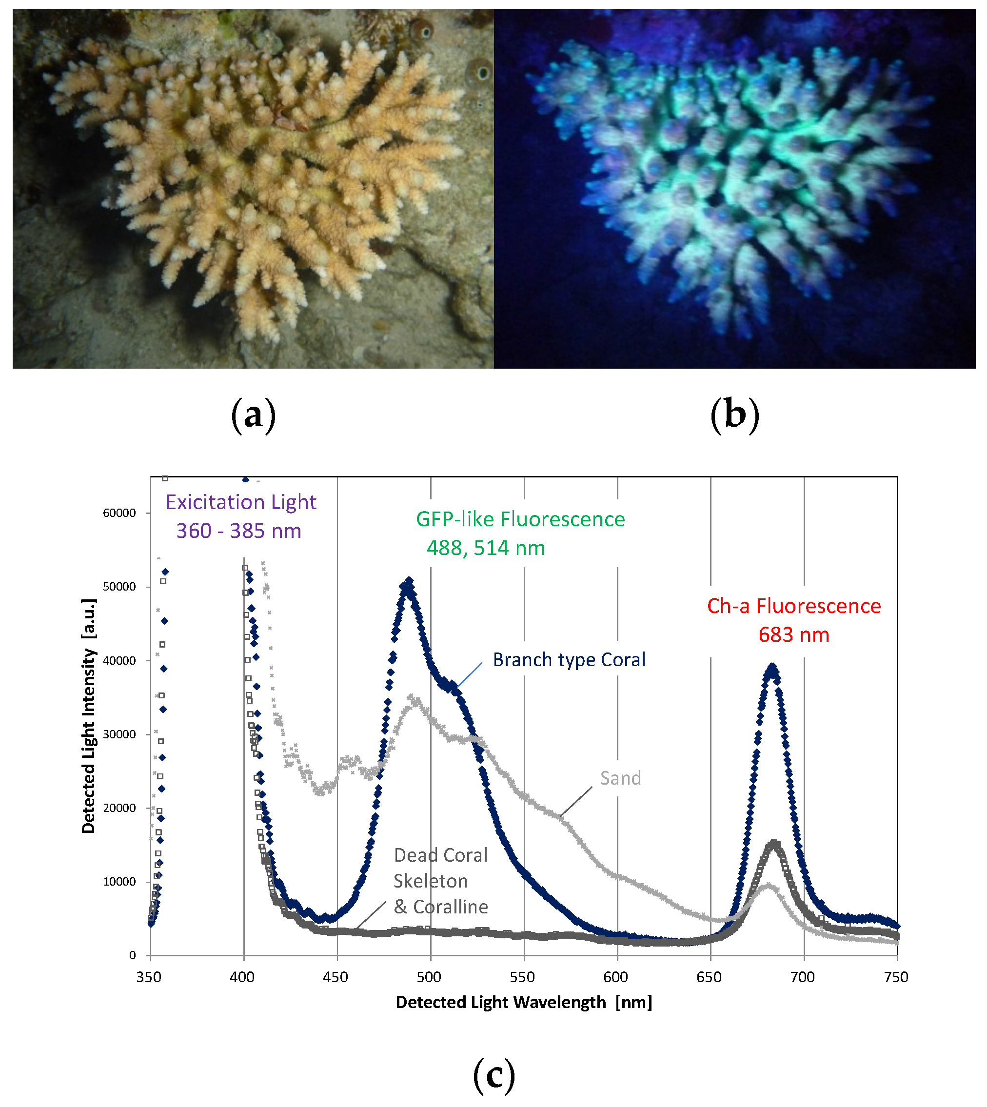
2.1. Fluorescence Properties of Corals

UV—excited fluorescence properties of a coral colony are confirmed in this work by imaging and spectrometry on Taketomi Island, Okinawa, Japan. The left and central panels of Figure 1 are the night-time underwater photographs of a branch-type coral colony at Taketomi Island, taken under white and UV light illumination, respectively. The color of the fluorescence differs in different parts of the branches. The right panel of Figure 1 shows the UV—excited fluorescence spectrum of the same branch-type coral measured by an underwater UV—excited spectrometer [13]. The intensity of the coral fluorescent proteins peaks at 488 and 514 nm. There is also an excitation light peak at 375 nm and a chlorophyll-a peak at 683 nm.

Figure 1. (a) Night-time white light-illuminated photograph; (b) UV—excited fluorescence photograph; and (c) UV—induced fluorescence spectrum of the same coral colony as compared with those of sand and CCA.

Figure 1. (a) Night-time white light-illuminated photograph; (b) UV—excited fluorescence photograph; and (c) UV—induced fluorescence spectrum of the same coral colony as compared with those of sand and CCA.

The viability of a specific coral colony can be judged from a time series of fluorescence images. Figure 2 presents underwater photographs taken during the day-time and at night-time under UV light. These images were taken several months apart. While the viability of the colony is difficult to judge from the underwater photographs taken under sunlight, the night-time fluorescence photographs clearly reveal the degradation of the colony over time. The coral colony fluoresced until October 2010, and fluorescence ceased after December 2010. We therefore infer that this colony died between October and December of 2010.

Although observing the night-time UV—excited fluorescence offers an effective coral colony viability check, the observation area is much more limited than in day-time underwater observation.

Figure 2. Day-time photographs (upper four photographs) and night-time UV—induced fluorescence photographs (lower four photographs) of the same damaged coral colony in July, October, December 2010, and September 2011. The fluorescence property of this coral colony disappeared due to dissolution of fluorescent proteins between October and December 2010.

Figure 2. Day-time photographs (upper four photographs) and night-time UV—induced fluorescence photographs (lower four photographs) of the same damaged coral colony in July, October, December 2010, and September 2011. The fluorescence property of this coral colony disappeared due to dissolution of fluorescent proteins between October and December 2010.

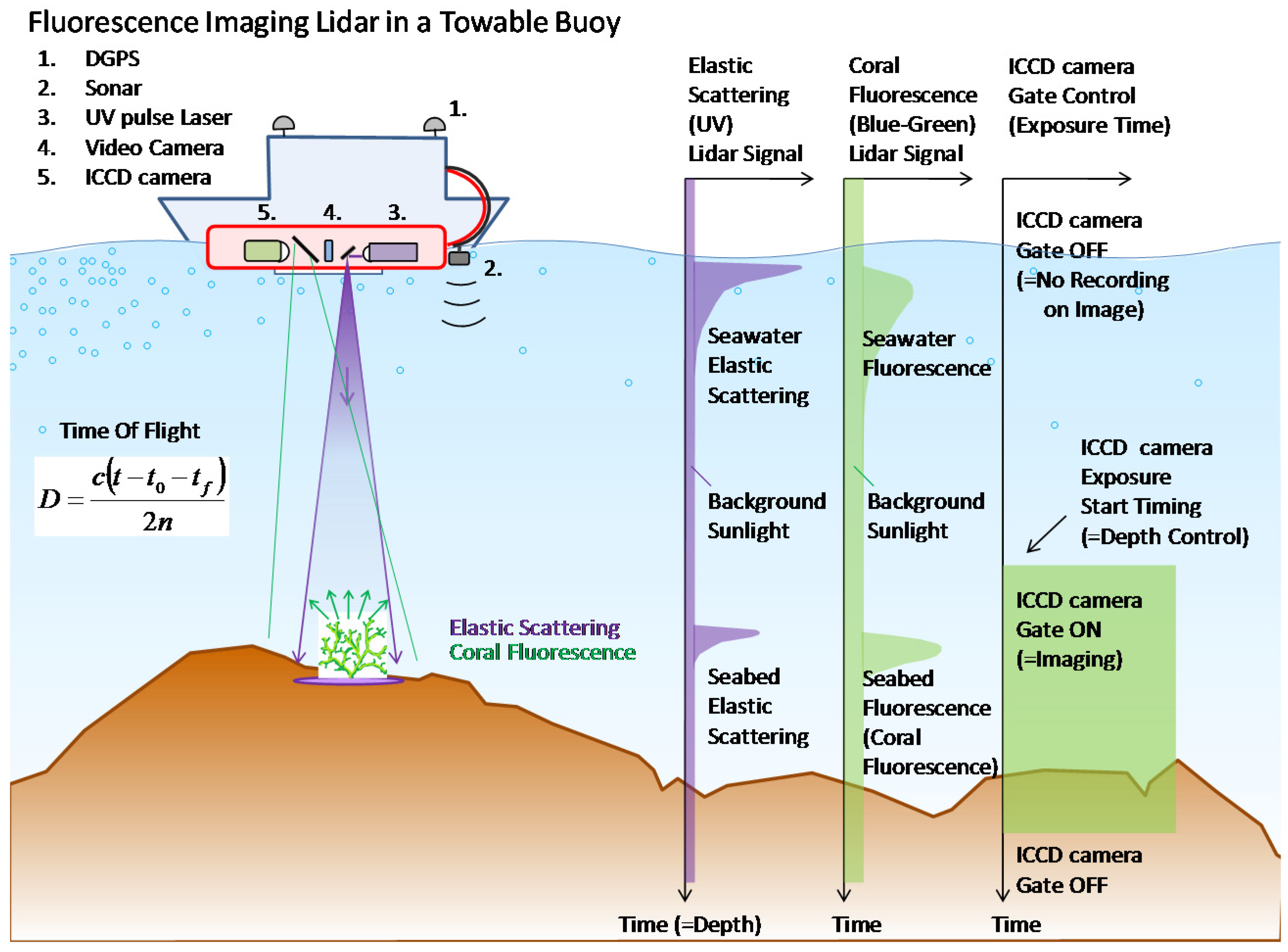
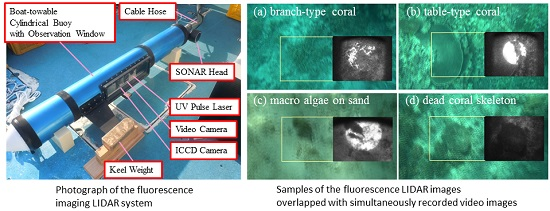
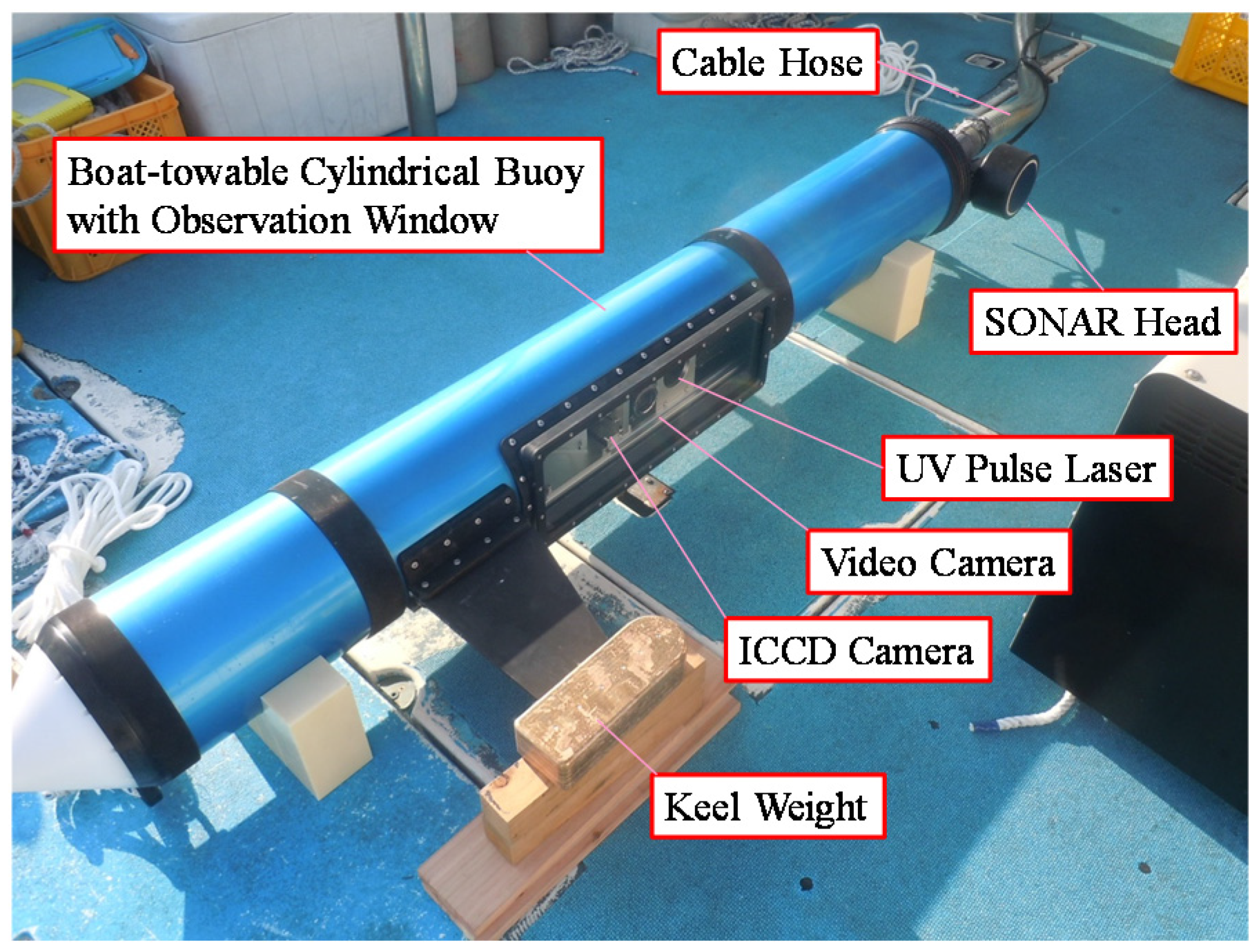
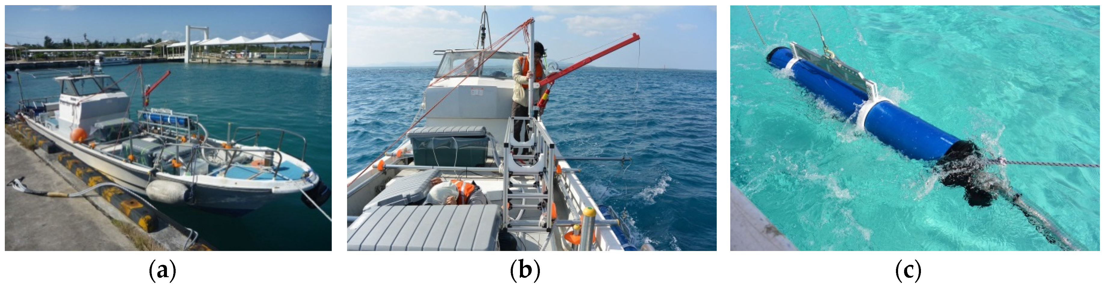
2.2. Fluorescence Imaging LIDAR System

Night-time fluorescence imaging of corals under UV light avoids background sunlight in the observed images. However, large—area boat observations must be conducted in the day-time because the boat operator must confirm the sea traffic safety and sea bottom conditions in shallow sea areas. Therefore, a fluorescence imaging LIDAR system has been developed for day-time observations of coral fluorescence images.

LIDAR is an active remote sensing technique mainly based on a pulsed laser. The fluorescence LIDAR employs “short cut” optical filters in the receiver system and observes only those wavelengths from the target that are longer than the laser wavelength. The detection time of the fluorescence is obtained by summing the pulsed laser irradiance timing t₀, the time of flight nD/c from the laser to the target, the fluorescence emission time of the laser—induced target t_f, and the time of flight from the target to the receiver (also given by nD/c).

$$t=t_0+2D\frac{n}{c}+t_f$$

(1)

where c is the light speed in vacuum, n is the absolute refractive index of seawater, and D is the distance between the LIDAR system and the target. The fluorescence emission time of the laser—induced target t_f is approximately 1–3 ns [14].

In this system, the wavelength and pulse width of the UV—pulsed laser is 355 nm and approximately 9 ns, respectively, and the exposure time of the two—dimensional image—intensified CCD (hereafter ICCD) camera is approximately 100 ns. To suppress the effect of background sunlight, we set a very—short exposure time. The very—short duration of the laser irradiation avoids image blurring under the boat propulsion and motion. In addition, the influence of the laser backscattering light from seawater is reduced by adjusting the gate open timing of the ICCD camera, depending on Equation (1). Thus, this system obtains clear fluorescent seabed images during the day-time without mechanical laser scanning. The fluorescence imaging LIDAR system during the observation is schematized in Figure 3.

Figure 3. Schematic of the fluorescence imaging LIDAR system.

Figure 3. Schematic of the fluorescence imaging LIDAR system.

The main devices of the system are installed in a towable buoy (diameter and length of 200 mm and 2 m, respectively) with an observation window. The moving observation is achieved by a boat—towing operation. Bathymetry is obtained by a Sound Navigation and Ranging (hereafter SONAR) sensor installed in the out—front of the buoy, and the boat is equipped with a three—antenna differential GPS (hereafter DGPS) sensor for position and boat heading information. The positioning error is approximately 1 m, and it realize the repetitive LIDAR observation of a coral colony. A photograph of the buoy is shown in Figure 4, and the system specifications are listed in Table 1.

Figure 4. Photograph of the fluorescence imaging LIDAR system installed in a boat—towable cylindrical buoy with an underwater observational window.

Figure 4. Photograph of the fluorescence imaging LIDAR system installed in a boat—towable cylindrical buoy with an underwater observational window.

Table 1. Specifications of the fluorescence imaging LIDAR system.

UV—pulsed Laser (Quantel CFR400)	Type	neodymium-doped yttrium aluminium garnet (Nd:YAG)
	Wavelength	355 nm
	Energy	90 mJ/pulse
	Pulse Width	9 ns
	Repetition	1–5 Hz (adjustable)
	Spread Angle	45 to 350 mrad (adjustable)
Gated ICCD Camera (Hamamatsu Photonics C10054-22) Collective Lens (Fujinon C22-17A-M41)	ICCD Type	Image—intensifiedCCD with Gate function of usual OFF
	Quantum Efficiency	50% (Max)
	Image Gain	5 × 106 (Max)
	ICCD Wavelength Range	280–720 nm
	Max. sensitive wavelength	530 nm
	CCD number of pixels	768 × 494
	Lens Diameter	70 mm
	Lens Wavelength Range	407 nm–Visible
	Field of View	35 to 660 mrad (adjustable)
Video Camera (Sony HDR-CX560V)	Type	1/3 inch complementary metal–oxide–semiconductor (CMOS)
	Field of View	90 to 1050 mrad (adjustable)
	CMOS pixel size	6.14 × 106 pixel (16:9)
DGPS Sensor (Septentrio PolaRx2e@)	Type	Single frequency, 3 antenna
	Position Accuracy	1 m
	Attitude Accuracy	5 mrad
SONAR Depth Sounder (Tamaya Technics TDM-9000B)	Frequency	200 kHz
	Spread Angle	200 mrad
	Observation Range	1 to 100 m
	Depth Accuracy	0.1 m
Towable Buoy	Diameter	200 mm
	Length	2 m
	Observation Window	Pyrex–reinforced glass

Table 1. Specifications of the fluorescence imaging LIDAR system.

UV—pulsed Laser (Quantel CFR400)	Type	neodymium-doped yttrium aluminium garnet (Nd:YAG)
	Wavelength	355 nm
	Energy	90 mJ/pulse
	Pulse Width	9 ns
	Repetition	1–5 Hz (adjustable)
	Spread Angle	45 to 350 mrad (adjustable)
Gated ICCD Camera (Hamamatsu Photonics C10054-22) Collective Lens (Fujinon C22-17A-M41)	ICCD Type	Image—intensifiedCCD with Gate function of usual OFF
	Quantum Efficiency	50% (Max)
	Image Gain	5 × 106 (Max)
	ICCD Wavelength Range	280–720 nm
	Max. sensitive wavelength	530 nm
	CCD number of pixels	768 × 494
	Lens Diameter	70 mm
	Lens Wavelength Range	407 nm–Visible
	Field of View	35 to 660 mrad (adjustable)
Video Camera (Sony HDR-CX560V)	Type	1/3 inch complementary metal–oxide–semiconductor (CMOS)
	Field of View	90 to 1050 mrad (adjustable)
	CMOS pixel size	6.14 × 106 pixel (16:9)
DGPS Sensor (Septentrio PolaRx2e@)	Type	Single frequency, 3 antenna
	Position Accuracy	1 m
	Attitude Accuracy	5 mrad
SONAR Depth Sounder (Tamaya Technics TDM-9000B)	Frequency	200 kHz
	Spread Angle	200 mrad
	Observation Range	1 to 100 m
	Depth Accuracy	0.1 m
Towable Buoy	Diameter	200 mm
	Length	2 m
	Observation Window	Pyrex–reinforced glass

During the observation, several conditions are manually adjusted by the operator on the boat, depending on the depth, transparency, bottom sediment and other parameters of the observation point. These conditions are the laser spread angle, FOV of the ICCD camera, time delay between the pulsed laser injection and the exposure gate open, and the gain of the ICCD camera. The buoy is connected to the boat by a watertight hose, and the electric generator, electric parts of the laser, and other electrical equipment are installed on the boat.

3. Results

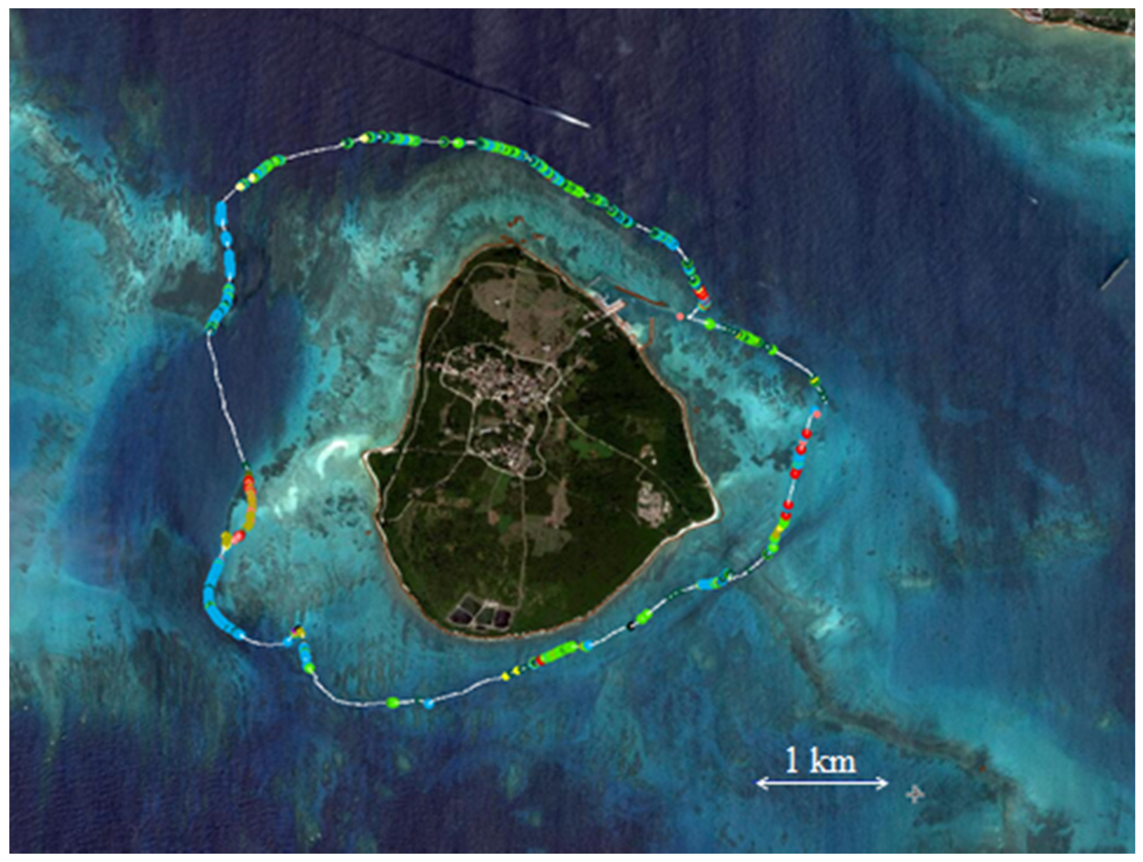
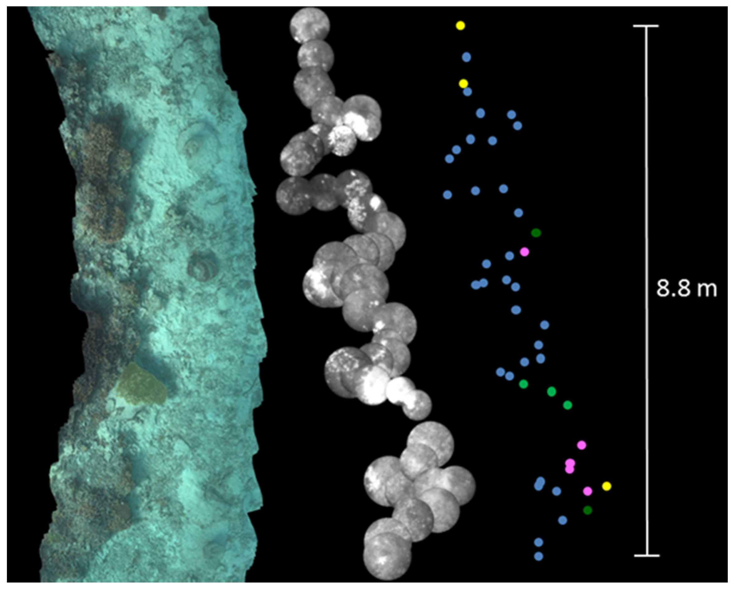
3.1. Long Line Observation

Coral observations were conducted by this system at Taketomi Island, Okinawa, Japan (24.33°N, 124.09°E) on 24 January 2015. A large number of fluorescence images of the seabed in the shallow coral reef sea area were successfully obtained. Passive seabed images, boat position data (accurate to 1 m), and bathymetry data (accuracy to 0.1 m) were simultaneously recorded using a video camera, DGPS, and SONAR, respectively. Photographs of the observation are shown in Figure 5. Representative fluorescent images, overlapped with simultaneous video images, are presented in Figure 6. The fluorescence LIDAR image has enough resolution to recognize a coral colony. The data analyst distinguished among branch—type coral, table—type coral, sea algae, sand, and other features from their target shapes in the video and fluorescence images. In addition, when the target is coral, the fluorescent image contrast provides a viability check. Therefore, two—dimensional high resolution seabed images are important for eye judgement classification of substrates as shown in Figure 6a–d, and fluorescent images are useful supplementary information for corals as shown in Figure 6a,b,d. The approximately 10 m scale mosaic images are shown in Figure 7 with the data analyst’s classification.

Figure 5. Photographs of coral observation by the fluorescence imaging LIDAR system at Taketomi Island, Okinawa Japan. (a) Standby condition for cruising to the observation point; (b) The boat during the coral observation; (c) The towable buoy during the coral observation.

Figure 5. Photographs of coral observation by the fluorescence imaging LIDAR system at Taketomi Island, Okinawa Japan. (a) Standby condition for cruising to the observation point; (b) The boat during the coral observation; (c) The towable buoy during the coral observation.

Figure 6. Samples of the fluorescence LIDAR images overlapped with simultaneously recorded video images. (a) Branch-type coral; (b) table-type coral; (c) macro algae on sand; (d) dead coral skeleton. Fluorescence images recorded by the ICCD camera are shown in monochrome. Laser footprints are shown as centered circles. White portions inside the laser footprint indicate intensive fluorescence.

Figure 6. Samples of the fluorescence LIDAR images overlapped with simultaneously recorded video images. (a) Branch-type coral; (b) table-type coral; (c) macro algae on sand; (d) dead coral skeleton. Fluorescence images recorded by the ICCD camera are shown in monochrome. Laser footprints are shown as centered circles. White portions inside the laser footprint indicate intensive fluorescence.

The boat-based LIDAR observation around Taketomi Island was recorded at 5 Hz repetition. The boat track was approximately 14 km long, and the total observation time was approximately 3 h. Figure 8 shows the coral distribution map overlapped with a high—resolution satellite image (WorldView-3 28 November 2014). The data analyst checked the presence of substrate by eye judgment in 34,322 images obtained by the fluorescence imaging LIDAR system, along with the simultaneously recorded video, position, and depth data. The substrate features were categorized into branch-type coral, table-type coral, dead coral skeleton, dead coral skeleton rubble, sand, sea algae, sea grass, and various other features.

The images obtained by the fluorescence imaging LIDAR system were not blurred by the towed buoy motion. However, in deep or poorly transparent sea areas, the fluorescence images of the seabed became hazy due to the attenuation and scattering of the UV laser light and fluorescent light along the path in the sea water. In these cases, the substrate is difficult to judge, so the data were excluded from the analysis and not plotted on the map. Therefore, the plots in Figure 8 guarantee the existence of live corals at the observed time and place, but absent plots do not guarantee the absence of corals. The live corals observed by the fluorescence imaging LIDAR system were distributed through approximate depths of 2–12 m, measured by the bathymetry SONAR. Comparisons with the satellite image clarified that the LIDAR data were located in the large coral reef area which includes the northern reef slope of Taketomi Island, and along the southern shipping route.

Figure 7. Comparison of the seabed mosaic of video images (Left), the seabed mosaic of fluorescence LIDAR images (Center), and the data analyst’s eye judgement classification of substrates (Right: $● \text{blue}$ circles: branch—type coral, $● \text{green}$ circles: table—type coral, $● \text{dark} \text{green}$ circles: coral observed at low-resolution, $● \text{yellow}$ circles: juvenile coral or coral piece, $● \text{pink}$ circles: dead coral rubble).

Figure 7. Comparison of the seabed mosaic of video images (Left), the seabed mosaic of fluorescence LIDAR images (Center), and the data analyst’s eye judgement classification of substrates (Right: $● \text{blue}$ circles: branch—type coral, $● \text{green}$ circles: table—type coral, $● \text{dark} \text{green}$ circles: coral observed at low-resolution, $● \text{yellow}$ circles: juvenile coral or coral piece, $● \text{pink}$ circles: dead coral rubble).

Figure 8. Coral distribution observed by the boat-towed fluorescence imaging LIDAR on 24 January 2015, overlapped with a satellite image (WorldView-3 28 November 2014) of Taketomi Island, Okinawa, Japan. $● \text{blue}$ circles: branch-type coral, $● \text{green}$ circles: table-type coral, $● \text{dark} \text{green}$ circles: coral observed at low-resolution, $● \text{yellow}$ circles: juvenile coral or coral piece, $● \text{red}$ circles: dead coral, $● \text{pink}$ circles: dead coral rubble, $● \text{light} \text{brown}$ circles: sea algae, $● \text{dark} \text{brown}$ circles: sea grass.

Figure 8. Coral distribution observed by the boat-towed fluorescence imaging LIDAR on 24 January 2015, overlapped with a satellite image (WorldView-3 28 November 2014) of Taketomi Island, Okinawa, Japan. $● \text{blue}$ circles: branch-type coral, $● \text{green}$ circles: table-type coral, $● \text{dark} \text{green}$ circles: coral observed at low-resolution, $● \text{yellow}$ circles: juvenile coral or coral piece, $● \text{red}$ circles: dead coral, $● \text{pink}$ circles: dead coral rubble, $● \text{light} \text{brown}$ circles: sea algae, $● \text{dark} \text{brown}$ circles: sea grass.

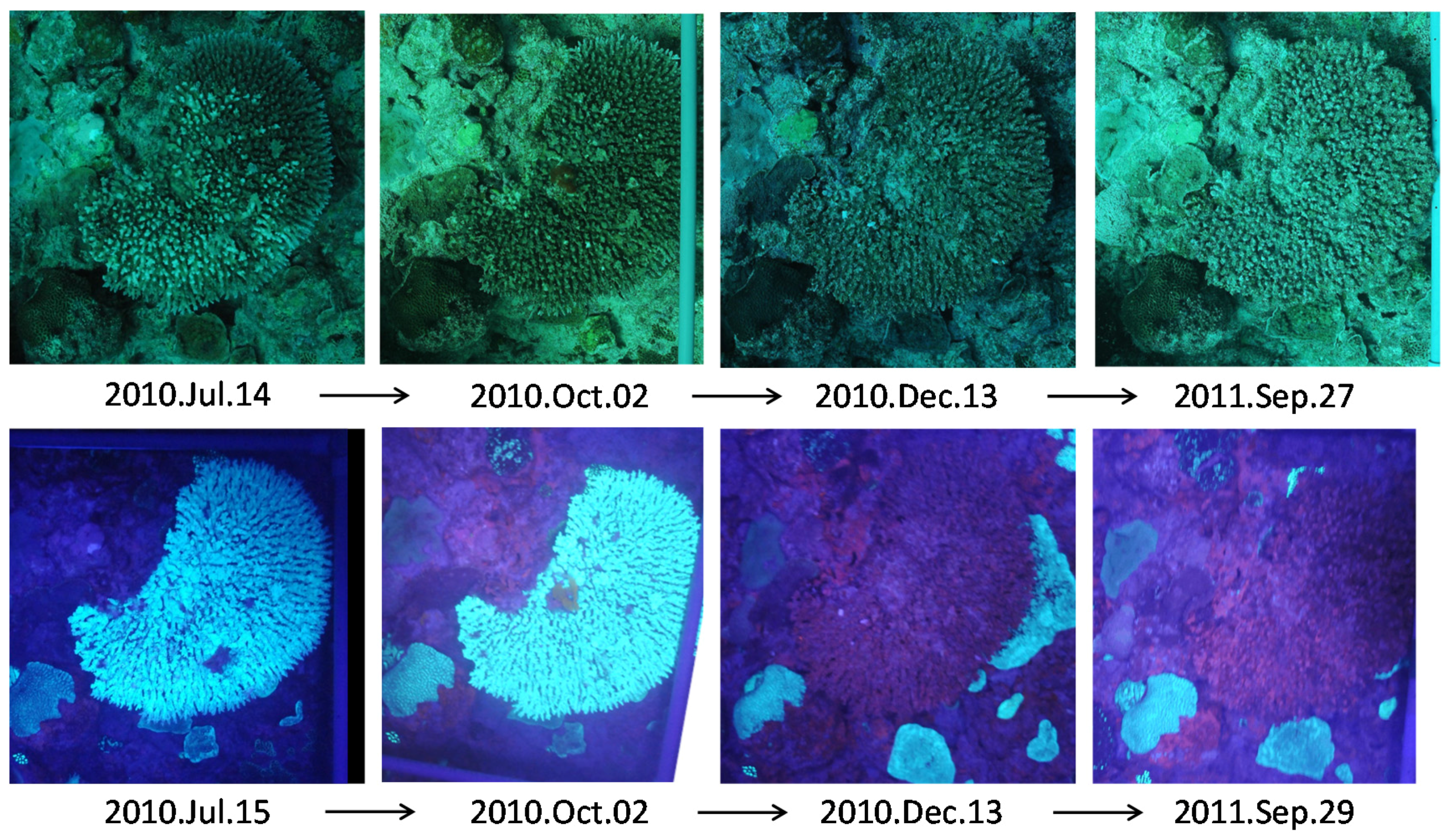
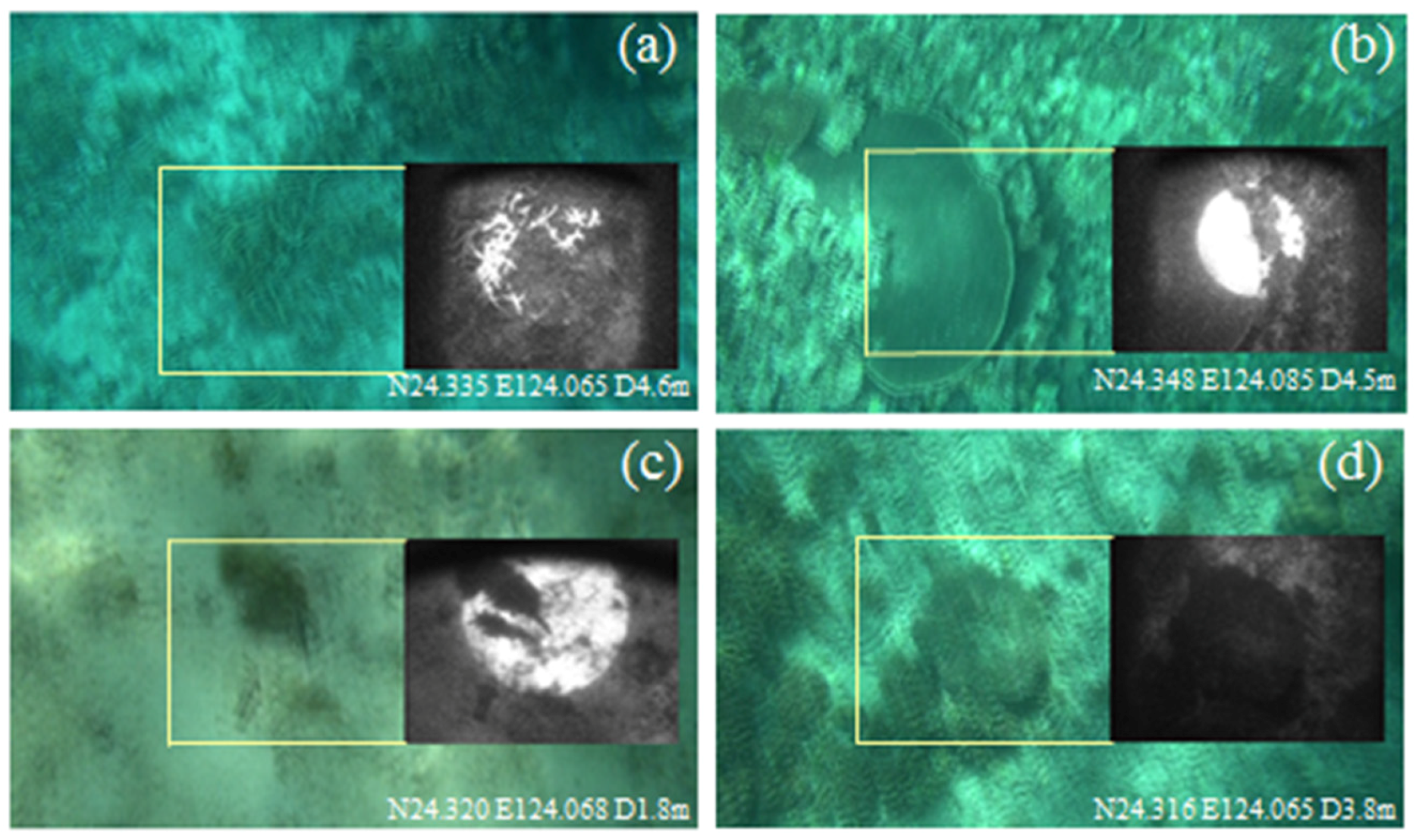
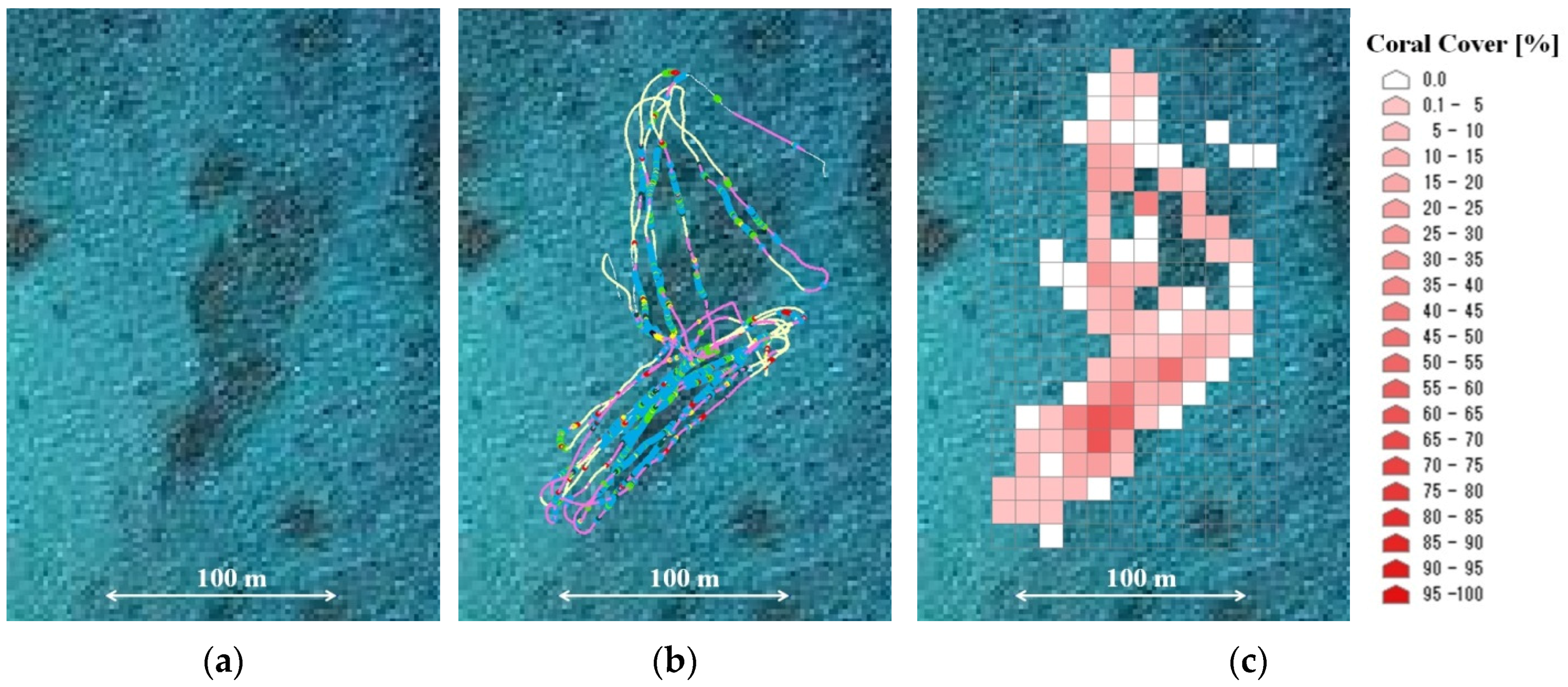
3.2. Coral Cover Observations

To calculate the coral cover from the observed data of the fluorescence imaging LIDAR, we must classify the seabed status into coral cover and other areas. For this purpose, we operated an intensive LIDAR observation in the shallow sea area (eastern sea area of Taketomi Island; depth below 6.5 m) in which the bottom sediment can be observed and determined with high confidence even if it is sand, rock, dead coral skeleton rubble, and other non-coral features. In approximately one hour, the LIDAR observation acquired 15,389 images.

Because we adjusted the laser spread angle and FOV of the ICCD camera, and the water depth varied during the operation, and the actual and recorded image sizes of the laser footprint on the seabed varied. To avoid this effect, we analyzed the center point of the circular laser footprint in each fluorescence image and judged the information as “ON” or “OFF” by eye from the shape and contrast of the substrate. Subsequently, the coral cover results are aggregated with the observation points over a position grid spanning 0.0001° latitude by 0.0001° longitude (approximately 11 m × 10 m), and the grids with more than 20 data of LIDAR observations are used for the coral cover calculation.

This analysis method involved the investigation of random sampled areas along the boat track rather the whole area. Though this approach simplifies the analysis, live corals are easily and reliably separated from other features in the fluorescent seabed images. The results of the coral cover analysis are shown in Figure 9. The total observed sea area comprised 98 grids (each approximately 113 m²), including one coral reef patch.

Figure 9. Coral cover observed by the fluorescence imaging LIDAR system on 24 January 2015. (a) High resolution satellite image (WorldView-3, 28 November 2014) of the LIDAR intensive observation area; (b) Coral distribution observed by the boat-towed fluorescence imaging LIDAR (colors are classified as in Figure 8); (c) Coral cover distribution.

Figure 9. Coral cover observed by the fluorescence imaging LIDAR system on 24 January 2015. (a) High resolution satellite image (WorldView-3, 28 November 2014) of the LIDAR intensive observation area; (b) Coral distribution observed by the boat-towed fluorescence imaging LIDAR (colors are classified as in Figure 8); (c) Coral cover distribution.

4. Conclusions

This paper describes the initial development and testing of a fluorescence imaging LIDAR system installed in a boat-towable buoy. Numerous fluorescence images of the seabed were successfully obtained around Taketomi Island, Okinawa, Japan. The UV—excited fluorescence provided a clear visual record of the coral colony condition or health. In addition, the system can be operated during the day-time, and the obtained fluorescence images were not blurred by the buoy propulsion and motion. The boat moved at approximately three knots, and the data recording repetition was 5 Hz. These operation conditions are practical for boat observations of regional coral reef areas. In addition, in a simplified coral cover analysis, we can determine the coral cover distribution in shallow coral reef areas (depth <6.5 m). As demonstrated in this study, boat observation using the fluorescence imaging LIDAR can be usefully combined with the high—resolution remote satellite images.

References

1. Wild, C.; Hoegh-Guldberg, O.; Naumann, M.S.; Colombo-Pallotta, M.F.; Ateweberhan, M.; Fitt, W.K.; Iglesias-Prieto, R.; Palmer, C.; Bythell, J.C.; Ortiz, J.-C.; et al. Climate change impedes scleractinian corals as primary reef ecosystem engineers. Mar. Freshw. Res. 2011, 62, 205–215. [Google Scholar] [CrossRef]
2. Status of Coral Reefs of the World: 2008, Global Coral Reef Monitoring Network Report 2008. Available online: http://www.icriforum.org/sites/default/files/GCRMN_Status_Coral_Reefs_2008.pdf (accessed on 14 September 2015).
3. Hoegh-Guldberg, O. Climate change, coral bleaching and the future of the world’s coral reefs. Mar. Freshw. Res. 1999, 50, 839–866. [Google Scholar] [CrossRef]
4. Hoegh-Guldberg, O.; Mumby, P.J.; Hooten, A.J.; Steneck, R.S.; Greenfield, P.; Gomez, E.; Harvell, C.D.; Sale, P.F.; Edwards, A.J.; Caldeira, K.; et al. Coral reefs under rapid climate change and ocean acidification. Science 2007, 318, 1737–1742. [Google Scholar] [CrossRef] [PubMed]
5. Hedley, J.D.; Mumby, P.J. Biological and remote sensing perspectives of pigmentation in coral reef organisms. Adv. Mar. Biol. 2002, 43, 277–317. [Google Scholar] [PubMed]
6. Treibitz, T.; Neal, B.P.; Kline, D.I.; Beijbom, O.; Roberts, P.L.; Mitchell, B.G.; Kriegman, D. Wide field-of-view fluorescence imaging of coral reefs. Sci. Rep. 2015, 5, 7694. [Google Scholar] [CrossRef] [PubMed]
7. Okamoto, M.; Sato, T.; Morita, S. Basic coral distribution data for long term monitoring at Sekisei Lagoon. In Proceedings of the OCEANS 2000 MTS/IEEE Conference and Exhibition, Providence, RI, USA, 11–14 September 2000; pp. 1383–1387.
8. Alieva, N.O.; Konzen, K.A.; Field, S.F.; Meleshkevitch, E.A.; Hunt, M.E.; Beltran-Ramirez, V.; Miller, D.J.; Wiedenmann, J.; Salih, A.; Matz, M.V. Diversity and evolution of coral fluorescent proteins. PLoS ONE 2008, 3. [Google Scholar] [CrossRef] [PubMed]
9. Salih, A.; Trevor-Jones, A. Fluorescence census techniques for the early detection of coral recruits. Coral Reefs 2006, 25, 73–76. [Google Scholar]
10. Zawada, D.G.; Mazel, C.H. Fluorescence-based classification of caribbean coral reef organisms and substrates. PLoS ONE 2014, 9. [Google Scholar] [CrossRef] [PubMed]
11. Mazel, C.H.; Cronin, T.W.; Caldwell, R.L.; Marshall, N.J. Fluorescent enhancement of signaling in a mantis shrimp. Science 2004, 303, 51. [Google Scholar] [CrossRef] [PubMed]
12. Research on Cooperative Coral Monitoring for Environmental Impact Assessment of Ocean-Warming and Acidification. Available online: http://www.env.go.jp/earth/kenkyuhi/report/pdf/11_2_3.pdf (accessed on 30 December 2015).
13. Sasano, M.; Matsumoto, A.; Imasato, M.; Yamano, H.; Oguma, H. Coral observation by fluorescence imaging LIDAR on a glass-bottom boat. J. Remote Sens. Soc. Jpn. 2013, 33, 377–389. (In Japanese) [Google Scholar]
14. Gilmore, A.M.; Larkum, A.W.D.; Salih, A.; Itoh, S.; Shibata, Y.; Bena, C.; Yamasaki, H.; Papina, M.; van Woesik, R. Simultaneous time resolution of the emission spectra of fluorescent proteins and zooxanthellar chlorophyll in reef-building corals. Photochem. Photobiol. 2003, 77, 515–523. [Google Scholar] [CrossRef]