A Statistical Algorithm for Estimating Chlorophyll Concentration in the New Caledonian Lagoon

Abstract

Spatial and temporal dynamics of phytoplankton biomass and water turbidity can provide crucial information about the function, health and vulnerability of lagoon ecosystems (coral reefs, sea grasses, etc.). A statistical algorithm is proposed to estimate chlorophyll-a concentration ([chl-a]) in optically complex waters of the New Caledonian lagoon from MODIS-derived “remote-sensing” reflectance (R_rs). The algorithm is developed via supervised learning on match-ups gathered from 2002 to 2010. The best performance is obtained by combining two models, selected according to the ratio of R_rs in spectral bands centered on 488 and 555 nm: a log-linear model for low [chl-a] (AFLC) and a support vector machine (SVM) model or a classic model (OC3) for high [chl-a]. The log-linear model is developed based on SVM regression analysis. This approach outperforms the classical OC3 approach, especially in shallow waters, with a root mean squared error 30% lower. The proposed algorithm enables more accurate assessments of [chl-a] and its variability in this typical oligo- to meso-trophic tropical lagoon, from shallow coastal waters and nearby reefs to deeper waters and in the open ocean.

1. Introduction

New Caledonia is a South Pacific archipelago located between longitudes 162° and 169° and latitudes −23° and −19°. The New Caledonian lagoon, which extends over 24,000 km², contains one of the most extensive reef systems in the world. These systems exhibit exceptional diversity of coral and fish species and a continuum of habitats from mangroves to sea grasses [1]. UNESCO added the New Caledonia Barrier Reef to the World Heritage List on 7 July 2008 [2], emphasizing the importance of preserving such biodiversity sites.

However, this fragile environment is subject to both anthropic and environmental stresses. Nickel mining is the major sector of the economy in New Caledonia. The various islands contain about 10% of the world’s nickel reserves [3]. The massive erosion caused by the mineral extraction process produces mineral matter inputs into the coastal ecosystem, particularly during rainy events [4]. These coastal inputs sometimes lead to fish death, coral bleaching, etc. [5]. Thomas et al. quantified farm discharges and evaluated their impacts in the lagoon of New Caledonia [6] where chlorophyll-a concentration ([chl-a]) is generally lower than 1.2 µg·L⁻¹ except in bays subject to anthropogenic influences where [chl-a] may increase to 3.6 µg·L⁻¹ [7]. Acanthaster planci (a coral-eating starfish) proliferation is probably due to algae proliferation, which is itself due to increased anthropogenic inputs, and a recent study highlighted a link between Acanthaster outbreaks and ocean productivity, favored by upwelling increased due to wind forcing [8].

Such increases in chlorophyll (up to 2 µg·L⁻¹ observed in the South Western lagoon) are either linked to rain [9,10] or to other processes such as upwelling or tides [11,12], which were recently modelled [13,14]. Climate change is also a factor of stress for reefs and lagoon ecosystems. Increase of ocean temperature, acidity, overexposure to sunlight and decrease in salinity affect the rate at which lagoons lose or gain water from evaporation, precipitation, surface runoff, and exchange with the ocean, and therefore water quantity and quality. Disturbances and other stressors may act concomitantly, or even interact, at multiple spatial and temporal scales, with consequences already documented or expected for the physical structure, ecological properties, and social values associated with lagoons. Many coral reefs in the world already suffer from climate and anthropogenic changes. Since 1985, Great Barrier Reef in Australia has lost more than half of its coral meadows [5]. Coral bleaching events happened in 1998 and 2002: more than 60% of the coral populations were hit, and even though the situation improved after several weeks, about 10% of the population perished [5,15,16]. To avoid or to monitor such events, it is necessary to accurately assess water properties in terms of chemical, biogeochemical and thermal characteristics, among which is chlorophyll concentration, an indicator of phytoplankton biomass.

Empirical algorithms have been developed in order to predict [chl-a] from ocean color seen by satellites [17,18]. The NASA OC3 algorithm uses a relation between [chl-a] and logarithms of R_rs ratios. The relation used for MODIS imagery is a polynomial function of the maximum R_rs ratio in spectral bands centered on 443 and 555 nm and 488 and 555 nm. This algorithm is valid in oceanic waters where a change in [chl-a] mainly causes a shift in the blue to green water reflectance ratio [19]. By using a color index defined as the difference between R_rs in the green and a reference formed linearly between R_rs in the blue and in the red, [20] improved OC3 assessments in global ocean where [chl-a] is less or equal to 0.25 µg·L⁻¹. In coastal waters, the ratios used in these algorithms can vary due to the influence of other optical components (colored dissolved organic matter—CDOM—and suspended sediments) besides [chl-a], which may introduce large errors in [chl-a] retrievals from satellite data [21,22]. Recently, a round-robin exercise for MERIS was conducted for some coastal areas of the world including the Great Barrier Reef, giving clues for discrepancies noticed in optically complex waters [23]. In coastal waters with high [chl-a] (10 µg·L⁻¹), algorithms based on regressions between MODIS reflectance ratios and [chl-a] improved the [chl-a] estimates [24]. Supervised learning was also used to develop an algorithm adapted to a coastal eutrophic region (between 5 and up to 50 µg·L⁻¹ chl-a) [25,26]. Camps-Valls et al. [27] showed how to improve the use of Support Vector Regression (SVR) or Relevance Vector Machine (RVM) [28] to estimate oceanic [chl-a] from remote sensing.

Past inter-comparison studies [29,30] reported negative or positive biases in [chl-a] retrievals with OC3 applied in lagoon imagery of New Caledonia, leading us to investigate a new algorithm. Average depth is 25 m in the lagoon and waters are principally oligotrophic, with weak [chl-a] and turbidity [29,31]. The changing bathymetry, very variable bottom types, and the oligotrophic and shallow nature of these waters are sources of errors made with OC3 applied to MODIS data [29]. In such shallow waters, R_rs not only depends on the absorption and scattering properties of dissolved and suspending materials in the water column but also on the depth and reflectivity of the bottom [32]. Recently, an inversion method was developed for the lagoon waters of New Caledonia [33]. A recent study has shown that depth strongly influences [chl-a] assessments [34]. Moreover, the influence of attenuation on seabed reflectance and exact bathymetry retrievals has been defined for the New Caledonia lagoon [35]. Thus, NASA products based on OC3 are not adapted to New Caledonia coastal waters.

Another [chl-a] algorithm, OC5 [36], was tested for New Caledonian lagoon waters. However, OC5 was especially designed for the very turbid waters of the shallow Brittany coast or for Tunisian waters [37] with high [chl-a]. This means it is not well-suited for the oligotrophic waters of New Caledonia. Moreover OC5 sets a minimum [chl-a] value of 0.1 µg·L⁻¹, but lower values are sometimes encountered in the New Caledonia lagoon [38] (see also below).

A preliminary study [39], inspired from encouraging results described in [25,26,27,28], showed that a statistical approach could improve [chl-a] retrievals in coastal New Caledonia waters. Indeed, when using a statistical approach, we expect to take into account particularities of optical properties in the study region. Moreover, even though atmospheric correction algorithms are generally not accurate for coastal applications and could lead to large [chl-a] errors, a statistical approach could overcome such problems for our specific area. In this paper, we show how to design a semi-empirical algorithm for estimating [chl-a] in the New Caledonian lagoon from in situ data collected in the region in coincidence with MODIS data from 2002 to 2010 [38]. The resulting algorithm is compared with the NASA OC3 version 6. No comparison was done with the reflectance difference algorithm [20] because our focus is on lagoon waters. The addition of variables such as bathymetry [32,34] and coastal distance [7] is also tested in order to investigate their ability to improve [chl-a] retrievals.

2. Material and Methods

2.1. Data

Two databases are used in this study: world data from SeaWIFS Bio-optical Archive and Storage System (SeaBASS:[40]) and data collected in the New Caledonia area (NCDataBase). Each database contains in situ and MODIS R_rs values in several spectral bands centered on 412 nm, 443 nm, 488 nm, 531 nm, 555 nm, and 667 nm for NCDataBase [29,31,38] and 547 instead of 555 nm for SeaBASS [40,41]. All MODIS R_rs over New Caledonia in the NCDataBase were extracted from 2002 to 2010 [42]. When the two databases are merged, which we call Full DataBase (FDB), it is assumed that the 547 and 555 nm spectral bands give an equivalent signal, i.e., they are considered one category [20]. The NCDataBase contains bathymetry (in meters) and in situ [chl-a] (µg·L⁻¹) measured by fluorometry and spectrofluorometry [29,43]. Water samples were collected from a Niskin bottle at 2 m depth. SeaBASS contains in situ [chl-a] obtained by fluorometry and HPLC, but for consistency only fluorometric measurements were used, and bathymetry was extracted from each latitude-longitude of the measurements.

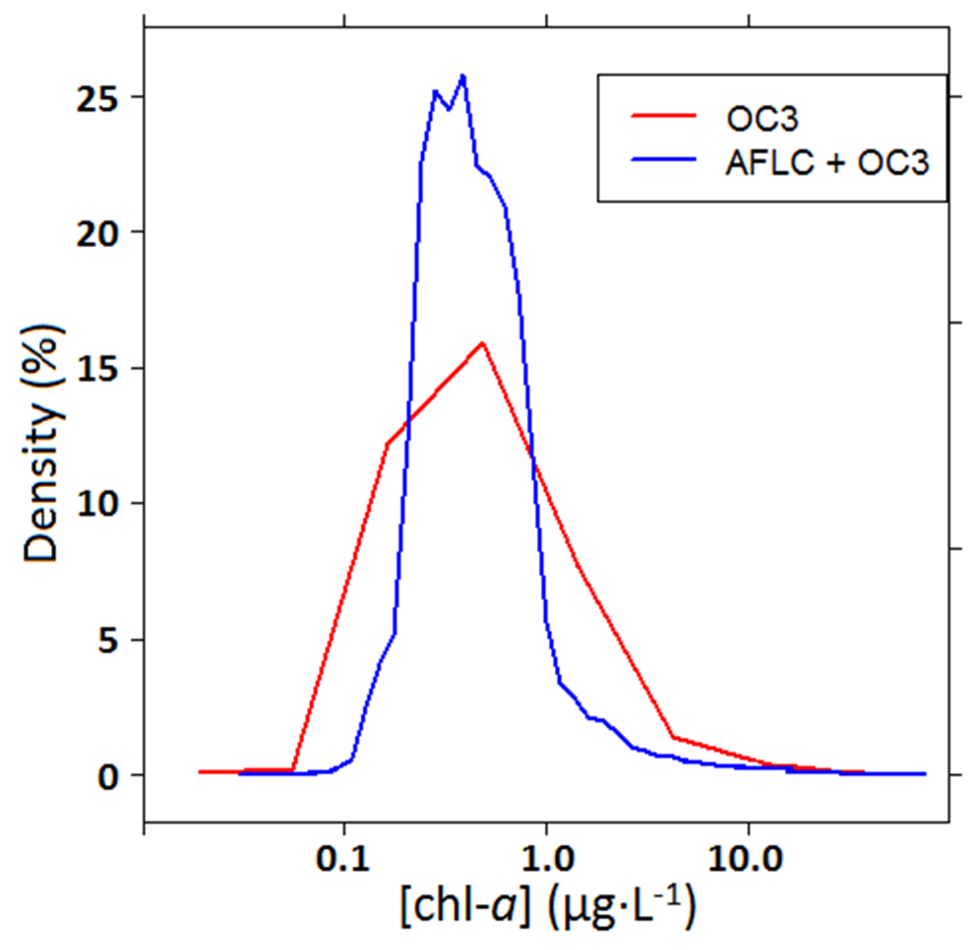
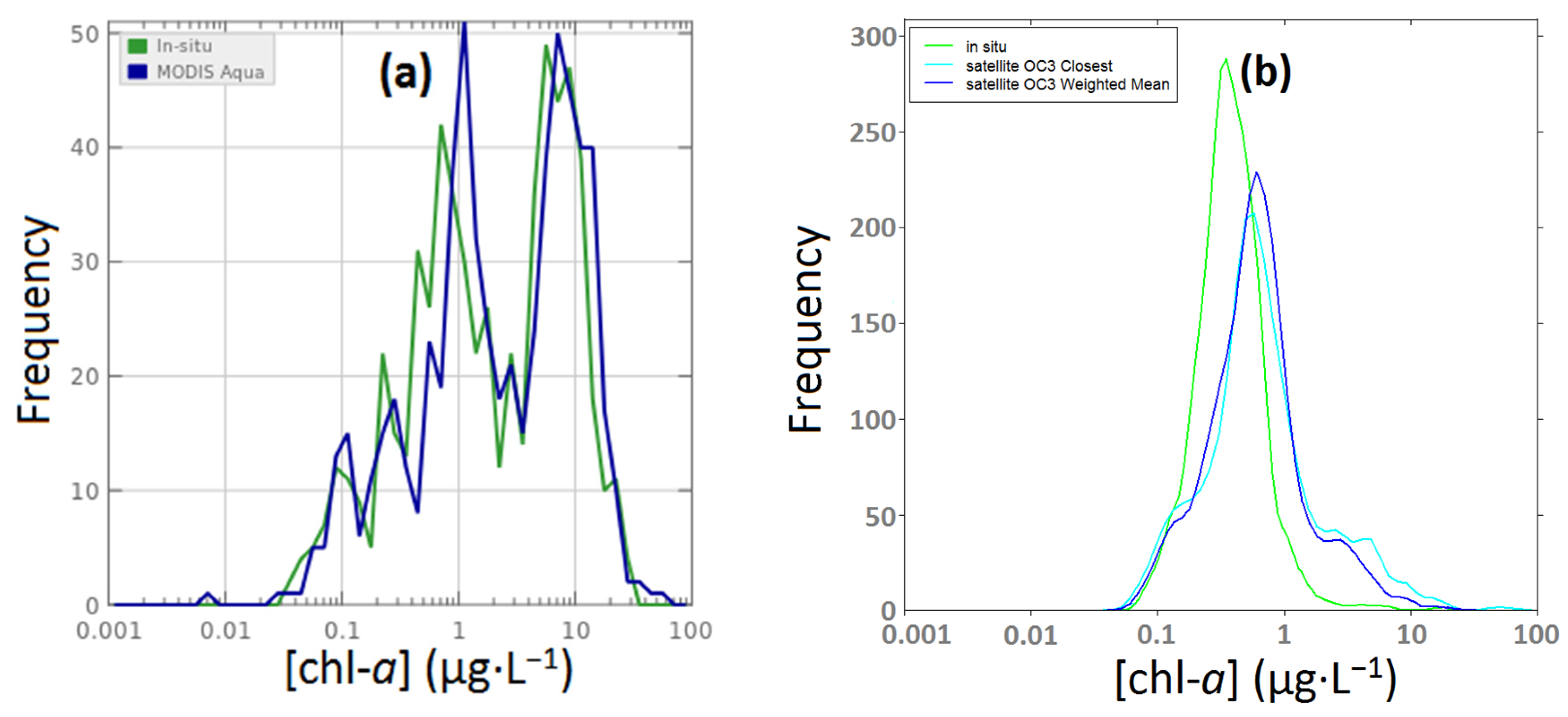
Figure 1a,b display the distribution of satellite and in situ [chl-a] in SeaBASS and NCDataBase, respectively. The SeaBASS data distribution is bi-modal, with separation at about 3 µg·L⁻¹. The two methods for satellite assessments (closest and weighted mean) are introduced in Section 2.2. When constructing the NCDataBase [43], all field measurements of [chl-a] by fluorometry collected from 1997 to 2010 during more than ten campaigns, mainly in the Southern lagoon [26], were selected with coincident MODIS R_rs. The full area extends from 165.95° to 168.65°E and from 24° to 19.99°S [38]. 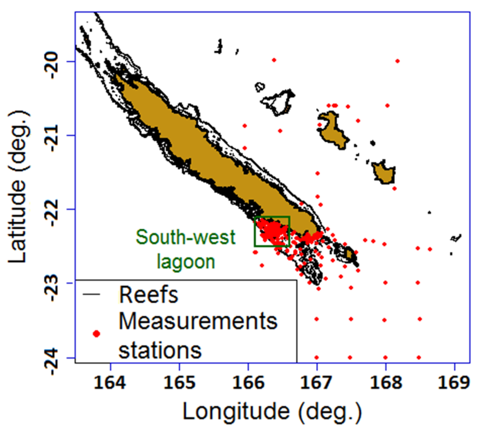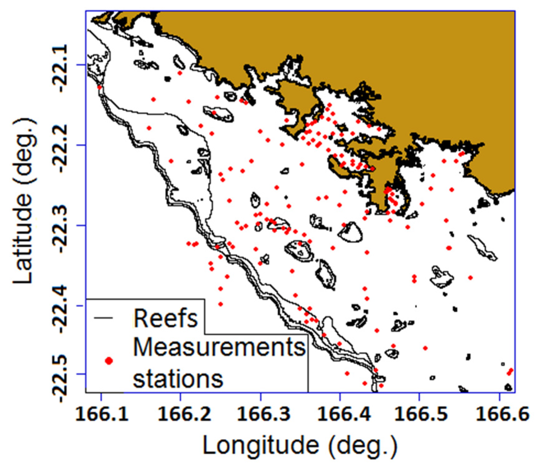Figure 2 and Figure 3 display measurement stations and Table 1 gives information about dates and campaigns used for the NCDataBase. Data were collected during each seasonal period for 13 years, which ensures a large range of situations. As several years and all seasons are sampled, we expect no bias due to El-Niño or La Niña event and seasonal variations.

Figure 1. (a) SeaBASS [chl-a] histogram (from the SeaBASS website): green line for in situ measurements and blue line for MODIS Aqua assessments; (b) NCDataBase [chl-a] histogram: green line for in situ measurements, cyan line for “OC3-Closest pixel” assessment and blue line for “OC3-Weight Mean” assessment.

Figure 1. (a) SeaBASS [chl-a] histogram (from the SeaBASS website): green line for in situ measurements and blue line for MODIS Aqua assessments; (b) NCDataBase [chl-a] histogram: green line for in situ measurements, cyan line for “OC3-Closest pixel” assessment and blue line for “OC3-Weight Mean” assessment.

Table 1. Sea campaigns from 1997 to 2010 in New Caledonia in [43].

Sea Campaign	Dates	Study Area
Camelia and Camecal (1–9)	21 Oct. 1997 to 27 Jun. 2003	South-West lagoon
Diapalis (1–9)	13 Oct. 2001 to 15 Oct. 2003	Loyalty Channel/Ouinné lagoon
Topaze 1–29	26 Apr.2001 to 26 Jan. 2004	South-West lagoon
Transects 1	1 Apr. 2003 to 10 Apr. 2003	South-West lagoon
Timeseries	12 Dec. 2001 to 22 Apr. 2003	South-West lagoon
Transects 2	4 May 2002 to 29 Feb. 2004	South-West lagoon
Southern and Northern 1 transect	21 Jun. 2003 to 7 Aug. 2003	South-West lagoon
Southern and Northern 2 transect	9 Nov. 2004 to 9 Dec. 2004	South-West lagoon
Bissecote	1 Feb. 2006 to 14 Feb. 2006	South-West lagoon
Echolag	14 Feb. 2007 to 5 Mar. 2007	Great South Lagoon
Zonalis	2 Mar. 2008 to 14 Mar. 2008	South of New Caledonia
Valhybio	22 Mar. 2008 to 8 Apr. 2008	LSO and GLS, offshore stations
ValhybioSM	27 Apr. 2008 to 21 Jul. 2010	Lagoon and offshore OC1 station

Table 1. Sea campaigns from 1997 to 2010 in New Caledonia in [43].

Sea Campaign	Dates	Study Area
Camelia and Camecal (1–9)	21 Oct. 1997 to 27 Jun. 2003	South-West lagoon
Diapalis (1–9)	13 Oct. 2001 to 15 Oct. 2003	Loyalty Channel/Ouinné lagoon
Topaze 1–29	26 Apr.2001 to 26 Jan. 2004	South-West lagoon
Transects 1	1 Apr. 2003 to 10 Apr. 2003	South-West lagoon
Timeseries	12 Dec. 2001 to 22 Apr. 2003	South-West lagoon
Transects 2	4 May 2002 to 29 Feb. 2004	South-West lagoon
Southern and Northern 1 transect	21 Jun. 2003 to 7 Aug. 2003	South-West lagoon
Southern and Northern 2 transect	9 Nov. 2004 to 9 Dec. 2004	South-West lagoon
Bissecote	1 Feb. 2006 to 14 Feb. 2006	South-West lagoon
Echolag	14 Feb. 2007 to 5 Mar. 2007	Great South Lagoon
Zonalis	2 Mar. 2008 to 14 Mar. 2008	South of New Caledonia
Valhybio	22 Mar. 2008 to 8 Apr. 2008	LSO and GLS, offshore stations
ValhybioSM	27 Apr. 2008 to 21 Jul. 2010	Lagoon and offshore OC1 station

Table 2 describes the content of the two databases in terms of [chl-a] values. In the NCDataBase (811 coincidences), we distinguish oceanic waters (bathymetry > 70 m, 159 coincidences) for which the bottom does not affect the water color, lagoon’s deep waters (20 m ≤ bathymetry ≤ 70 m, 352 coincidences) for which the bottom has a priori a little influence on the water color, and lagoon’s shallow waters (bathymetry ≤ 20 m, 300 coincidences) for which the bottom may strongly affect the water color [29]. Similarly, we distinguish waters according to bathymetry for SeaBASS even if the influence of bathymetry is probably not equivalent both in world data and NCDataBase (see Section 4.1). However, thereafter and especially during the construction of our algorithm, no distinction is made based on the depth of the station because the bathymetry was not found to be a good explanatory variable (see Section 4.3). Furthermore, we distinguish data according to [chl-a] values, since we will treat high values (>3 µg·L⁻¹) and low values (≤3 µg·L⁻¹) separately; see Section 2.3.

Figure 2. Visited stations in New Caledonia.

Figure 2. Visited stations in New Caledonia.

Figure 3. Visited stations in the south-west lagoon.

Figure 3. Visited stations in the south-west lagoon.

Table 2. Database description.

		[chl-a] (µg·L−1)
Data base	N	Min	Max	≤3 (%)	>3 (%)
FDB (NCDataBase + SeaBASS)	1378	0.03	38.07	81.28	18.72
NCDataBase (<20 m)	300	0.08	2.71	100	0
NCDataBase (20 m ≤ bathy ≤ 70 m)	352	0.11	3.70	99.53	0.47
NCDataBase (>70 m)	159	0.08	1.05	100	0
NCDataBase (total)	811	0.08	3.70	99.75	0.25
SeaBASS (<20 m)	262	0.37	38.07	13.36	86.54
SeaBASS (20 m ≤ bathy ≤ 70 m)	20	0.22	6.26	75.00	25.00
SeaBASS (>70 m)	285	0.03	13.18	91.58	8.42
SeaBASS (total)	567	0.03	38.07	54.85	45.15

Table 2. Database description.

		[chl-a] (µg·L−1)
Data base	N	Min	Max	≤3 (%)	>3 (%)
FDB (NCDataBase + SeaBASS)	1378	0.03	38.07	81.28	18.72
NCDataBase (<20 m)	300	0.08	2.71	100	0
NCDataBase (20 m ≤ bathy ≤ 70 m)	352	0.11	3.70	99.53	0.47
NCDataBase (>70 m)	159	0.08	1.05	100	0
NCDataBase (total)	811	0.08	3.70	99.75	0.25
SeaBASS (<20 m)	262	0.37	38.07	13.36	86.54
SeaBASS (20 m ≤ bathy ≤ 70 m)	20	0.22	6.26	75.00	25.00
SeaBASS (>70 m)	285	0.03	13.18	91.58	8.42
SeaBASS (total)	567	0.03	38.07	54.85	45.15

2.2. Match-Up

The in situ [chl-a] and R_rs data were matched with MODIS Aqua standard retrievals for NCDataBase at original resolution (1-km, non-gridded data) [41], as provided by the NASA Ocean Color Biology Processing Group (OBPG). The atmospheric correction scheme took into account non-black pixels in the near infrared, but no adjacency effects. SeaDAS flags were applied to the satellite data to eliminate situations with sun glint, large viewing zenith angle, high water turbidity, clouds, land, high top-of-atmosphere radiance, and stray light [42]. To assign a value to a station on a day, two methods were used. The first method consists in assigning the value of the closest pixel: the closest neighbor method (CL) [38,41]. The second method consists in averaging the values from neighboring pixels, using weights depending on the distance to the station: the weighted mean method (WMM) [38,41]. This was done for the spectral bands centered on 412, 443, 488, 531, 555 and 667 nm.

The match-ups from MODIS Aqua images were created using a 0.04° square (about 4 × 4 km²) centered on the visited station as in [41] and in a 5-day temporal window. The two aforementioned methods were compared. They were applied with a temporal window from 0-day to 5-day. Several indices were computed, namely the variation coefficient (VC), the normalized mean bias (NMB), mean normalized bias (MNB), and root mean square error (RMSE):

$$VC=\frac{\mathsf{\sigma }}{\overline{x}}$$

(1)

$$NMB=\frac{\overline{y}-\overline{x}}{\overline{x}}$$

(2)

$$MNB=\frac{1}{n}{\displaystyle \sum }_{i=1}^n\frac{y_i-x_i}{x_i}$$

(3)

$$RMSE=\sqrt{\frac{1}{n}{\displaystyle \sum }_{i=1}^n{\left(y_i-x_i\right)}^2}$$

(4)

where $n$ is the number of observations, $x_i$ is the $i^{th}$ observation of in situ parameter, $y_i$ is the $i^{th}$ observation of remote sensing parameter, $\overline{x}$ is the in situ parameter mean, $\overline{y}$ is the remote sensing measures mean and $\mathsf{\sigma }$ is the standard deviation of remote sensing measures.

Table 3 displays the comparison statistics for MODIS and in situ R_rs matched data. It highlights that RMSE is not affected by the temporal window with a difference lower than 0.001 both between 0-day CL and 5-day CL, and between 0-day WMM and 5-day WMM. The VC values are very close too (0.358 for 0-day WMM and 0.355 for 5-day WMM). Moreover, NMB and MNB are better with a 5-day window (from −0.266 for 0-day WMM to −0.204 for 5-day WMM for NMB, and from −0.171 for 0-day WMM to −0.101 for 5-day WMM for MNB). Thus using a 5-day temporal window does not affect much the accuracy of results to assess R_rs(443) retrievals and the WMM [29,38,41,43] provides the best performance. 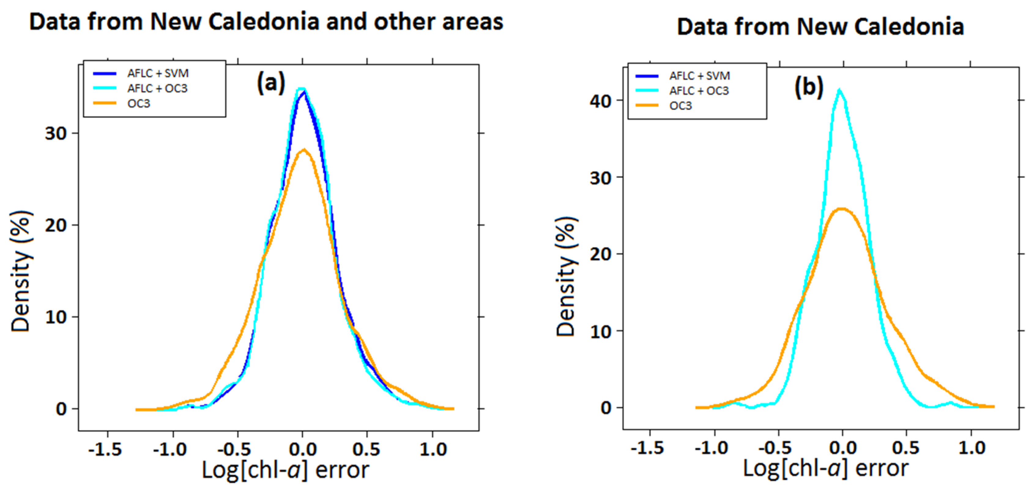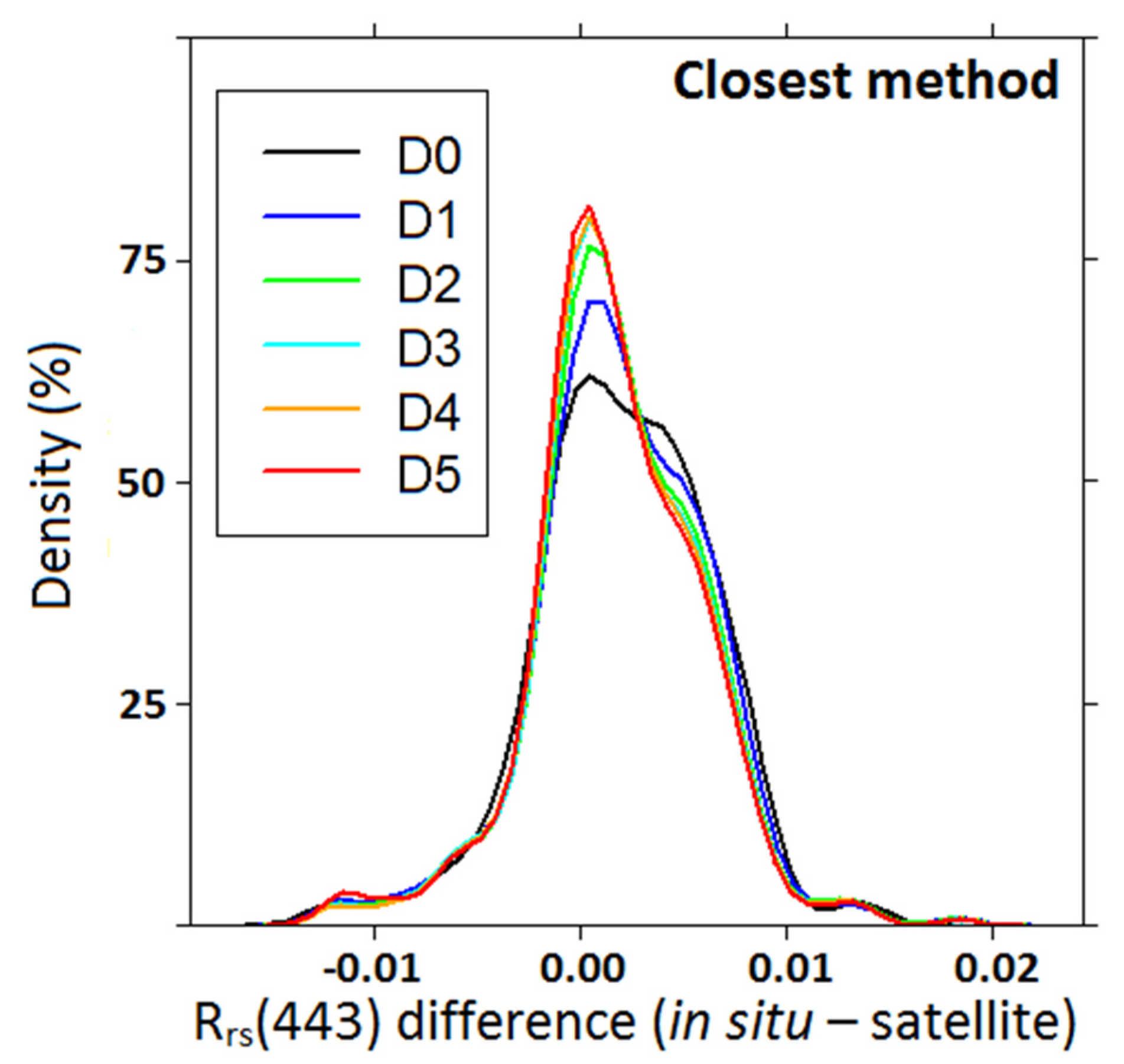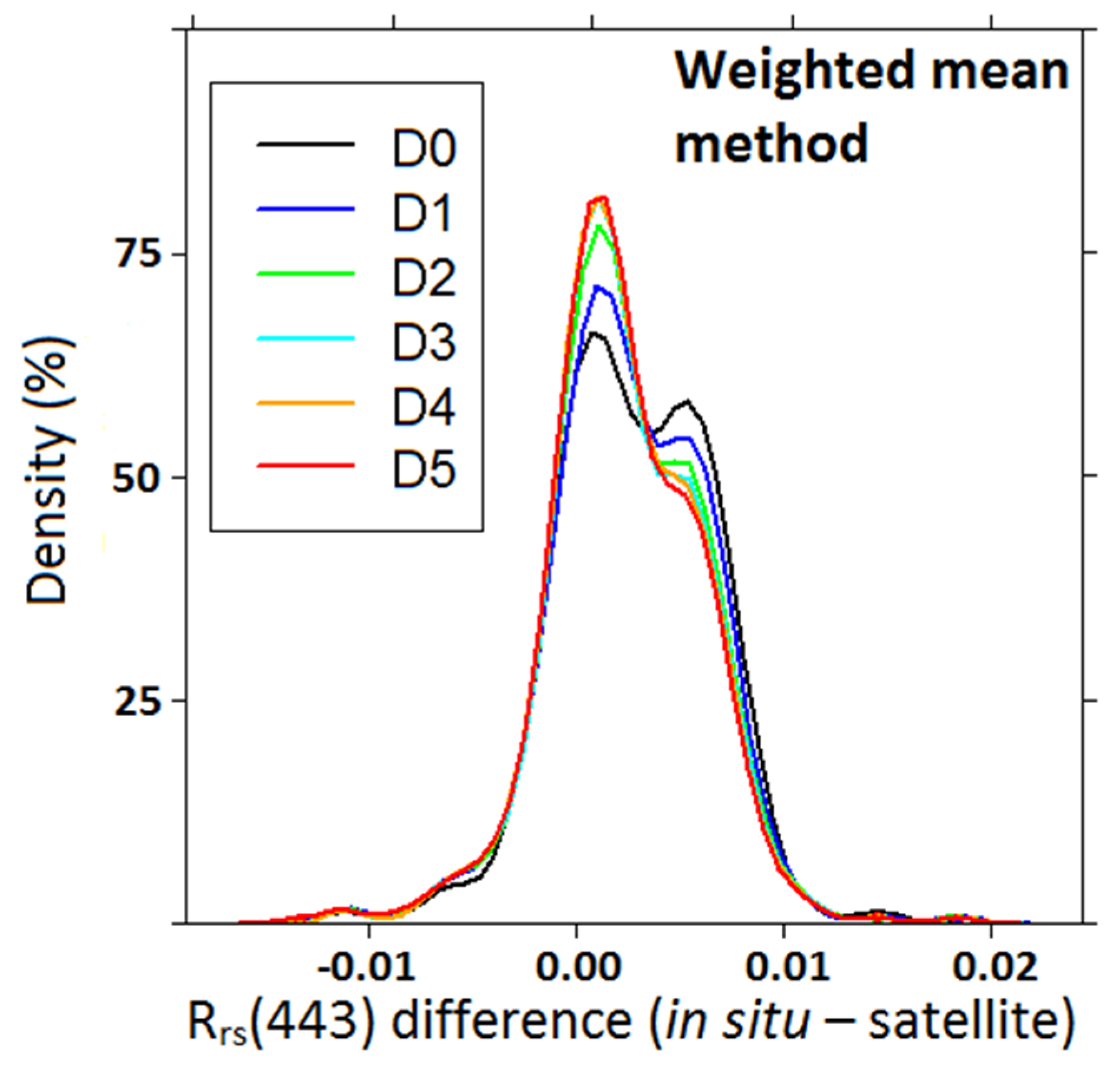Figure 4 and Figure 5 display error densities computed with the different in situ measurements and remote sensing assessments of R_rs(443) for the two methods. “Error densities” enable detection of whether an algorithm tends to overestimate, and whether errors are balanced or distributed around 0. They highlight that errors done with a 5-day temporal window are not much larger than errors made with a narrower window. This is explained by the fact that algorithm errors are similar to those introduces by temporal variability over a few days (see also Section 4.4). Moreover, our full dataset contains more than 86% of match-ups for which the temporal window is lower than or equal to 2 days. In order to keep a maximum of coincidences, we used the 5-day temporal window with the WMM. Since the weighted means method is more efficient, R_rs values were determined using this second method in our NCDataBase to investigate appropriate [chl-a] algorithms for the region.

Table 3. Different methods for generating R_rs(443) (sr⁻¹) match-ups in New Caledonian waters. Min, Max, Mean Median and RMSE are given in sr⁻¹.

Methods	n	Min	Max	Mean	Median	VC	NMB	MNB	RMSE
0-day CL	397	0.0000	0.0281	0.0062	0.0057	0.4298	−0.2700	−0.1633	0.0047
0-day WMM	397	0.0003	0.0213	0.0062	0.0058	0.3584	−0.2660	−0.1705	0.0044
1-day CL	752	0.0000	0.0281	0.0063	0.0059	0.3990	−0.2495	−0.1592	0.0047
1-day WMM	752	0.0003	0.0213	0.0065	0.0062	0.3452	−0.2311	−0.1454	0.0044
5-day CL	986	0.0000	0.0281	0.0062	0.0058	0.4096	−0.2289	−0.1274	0.0045
5-day WMM	986	0.0003	0.0213	0.0064	0.0061	0.3550	−0.2044	−0.1036	0.0042

Table 3. Different methods for generating R_rs(443) (sr⁻¹) match-ups in New Caledonian waters. Min, Max, Mean Median and RMSE are given in sr⁻¹.

Methods	n	Min	Max	Mean	Median	VC	NMB	MNB	RMSE
0-day CL	397	0.0000	0.0281	0.0062	0.0057	0.4298	−0.2700	−0.1633	0.0047
0-day WMM	397	0.0003	0.0213	0.0062	0.0058	0.3584	−0.2660	−0.1705	0.0044
1-day CL	752	0.0000	0.0281	0.0063	0.0059	0.3990	−0.2495	−0.1592	0.0047
1-day WMM	752	0.0003	0.0213	0.0065	0.0062	0.3452	−0.2311	−0.1454	0.0044
5-day CL	986	0.0000	0.0281	0.0062	0.0058	0.4096	−0.2289	−0.1274	0.0045
5-day WMM	986	0.0003	0.0213	0.0064	0.0061	0.3550	−0.2044	−0.1036	0.0042

Figure 4. Error densities between in situ measurements and satellite assessments for R_rs(443) at the same day (D0), and from a 1-day temporal (D1) window to a 5-day temporal window (D5). Closest neighbor method.

Figure 4. Error densities between in situ measurements and satellite assessments for R_rs(443) at the same day (D0), and from a 1-day temporal (D1) window to a 5-day temporal window (D5). Closest neighbor method.

Figure 5. Error densities between in situ measurements and satellite assessments for R_rs(443) at the same day (D0), and from a 1-day temporal window (D1) to a 5-day temporal window (D5). Weighted mean method.

Figure 5. Error densities between in situ measurements and satellite assessments for R_rs(443) at the same day (D0), and from a 1-day temporal window (D1) to a 5-day temporal window (D5). Weighted mean method.

2.3. Algorithm Steps

Our goal was to find an algorithm allowing good [chl-a] assessments in the lagoon of New Caledonia from the ocean color imagery acquired by MODIS. When creating the models, explanatory variables for assessing in situ [chl-a] are satellite R_rs. This is a different approach from the OC* algorithms from NASA, which use in situ R_rs as explanatory variables. The statistical study was conducted without a priori knowledge, i.e., all potentially explanatory variables (R_rs in the various spectral bands) were taken in account.

As indicated in Table 2, there are few data with high [chl-a] (>3 µg·L⁻¹) in the NCDataBase. As a result, the algorithm built from the NCDataBase will not be adapted to cases where the [chl-a] is high. The steps to get an algorithm adapted to New Caledonia are the following: (1) using the NCDataBase, determine a model for low [chl-a] (AFLC), i.e. a well-suited model for waters having low [chl-a]; (2) using the SeaBASS database, determine a model for waters with high [chl-a] (AFHC); (3) using the two merged databases, determine a criterion to distinguish low and high [chl-a]; and (4) implement a continuous connection between the models for low and high [chl-a].

Step 1 consists in determining which variables can give a good [chl-a] estimate. As variables are generally not independent, the support vector machine (SVM) method was used to select the best set of explanatory variables [26,28,44]. This kernel method finds the best regression through optimality criteria even if it means increasing the dimension of the variable space. Note that choosing SVM parameters is easier than with a neural network, for which the architecture can be very complex and hard to interpret. A bootstrap with fifty random draws was performed to determine the best parameters. On each draw, each combination of the explanatory variables was used to create and test a model. The number of all the combinations with six variables (R_rs(412), R_rs(443), R_rs(488), R_rs(531), R_rs(555) and R_rs(667)) is 63 (${{\displaystyle \sum }}_{i=1}^6\left(\begin{array}{c}6\\ i\end{array}\right)=63$). When a model formed with many variables gave results equivalent to a model formed with fewer explanatory variables, the model with fewer variables was chosen. For each of these 63 models, 50 RMSE values, one per sample, were computed. Results were compared by calculating averages, confidence intervals of RMSE averages, and by testing the equality of means. As computed averages did not follow a Normal Law, the Kruskal-Wallis test of means comparison was applied. For both the SeaBASS and NCDataBase combined, the best results were obtained with R_rs(443), R_rs(488) and R_rs(531). Once the best predictors were known, relations, such as a linear or a log regression, between [chl-a] and predictors and ratios of predictors were sought, with a method similar to the previous one: using bootstrap with 50 draws. With results statistically equivalent on test samples between the best SVM and a simpler relation, the simpler relation was selected.

In Step 2, only data with high [chl-a] were kept to build a specific model for [chl-a] greater than 3 µg·L⁻¹. A SVM model was built with a similar method as in Step 1. The predictive variables are the R_rs in the five spectral bands centered on 412, 443, 488, 531, and 555 nm. This SVM model was compared to OC3. The best model between this SVM and OC3 was chosen to complete the algorithm for high [chl-a].

Step 3 consists in determining from MODIS R_rs if the [chl-a] is high or low. In this step, two methods were tested to determine what MODIS color ranges are linked to a high or a low [chl-a]: SVM (as a classifier) and decision tree. As explained in more detail later (Section 4.1), the decision tree was preferred to the SVM because of its practicality. Indeed, only the ratio $R_{rs}\left(488\right)/R_{rs}\left(555\right)$ is used to determine which group of [chl-a] should be linked to a MODIS color.

For Step 4, several kinds of continuous connections, with weight functions, between the AFHC and the AFLC were tried: linear, quadratic, root squared, logarithmic, exponential, and arc-tangential. Equations (5.1)–(5.4) describe some weight functions with $s$ the threshold determining the limit between high and low [chl-a], $\epsilon \in \left]0;s\right[$ the tolerance used to set the transition interval width, $a=s- \epsilon$ the inferior bound of the transition interval, $b=s+\epsilon$ the superior bound of the transition interval, and $x$ is the variable which represents the ratio $R_{rs}\left(488\right)/R_{rs}\left(555\right)$.

$$\begin{array}{cc}\text{Linear:}& f\left(x\right)= \{\begin{array}{c}0 when x \in \left[0;a\right]\\ \frac{x-a}{b-a} when x \in \left]a;b\right[\\ 1 when x \ge b\end{array}\end{array}$$

(5.1)

$$\begin{array}{cc}\text{Quadratic:}& f\left(x\right)= \{\begin{array}{c}0 when x \in \left[0;a\right]\\ {\left(\frac{x-a}{b-a}\right)}^2 when x \in \left]a;b\right[\\ 1 when x \ge b\end{array}\end{array}$$

(5.2)

$$\begin{array}{cc}\text{Square root:}& f\left(x\right)= \{\begin{array}{c}0 when x \in \left[0;a\right]\\ \sqrt{\frac{x-a}{b-a}} when x \in \left]a;b\right[\\ 1 when x \ge b\end{array}\end{array}$$

(5.3)

$$\begin{array}{cc}\text{Arc-tangential:}& f\left(x\right)= \{\begin{array}{c}0 when x \in \left[0;a\right]\\ {\tan }^{-1}\left(\left[\frac{1}{b-x}- \frac{1}{x-a}\right]\frac{b-a}{s}\right)/\pi + 1/2 when x \in \left]a;b\right[\\ 1 when x \ge b\end{array}\end{array}$$

(5.4)

Given a value of the ratio $R_{rs}\left(488\right)/R_{rs}\left(555\right)$, the weight function $f$ is applied to the value determined by the AFLC algorithm, and the weight function $1-f$ is applied to the value determined by the AFHC (SVM or OC3).

We also tested a general SVM (SVMg) from the merged NCDataBase and SeaBASS database, built without differentiating between the two [chl-a] groups. For this SVMg construction, we used the bootstrap method described before (selection with 50 random draws). Explanatory variables belonging to the model were selected with learning and test samples. The model with the lower RMSE on test samples was retained. In this SVM, the kernel is the radial basis kernel and predictors are R_rs channels 443, 531 and 555 nm. The SVMg and the “AFLC + AFHC” algorithms were also compared with OC3.

2.4. Statistical Tests

In order to verify the effectiveness of an algorithm without an overtraining effect, data were systematically divided into two samples: one learning sample to build the model, and one test sample on which the built model was applied and checked with indicators (specified after). The learning sample was constructed with 70% of the data and the test sample was formed with the remaining 30%. To maintain the proportions between high and low [chl-a] in each sample when the NCDataBase and SeaBASS database were merged, samples were obtained with “semi-random draws”, i.e., the dataset was partitioned into two groups (high and low [chl-a]) and then a random draw was made for each group. For model comparisons, we essentially used RMSE (Equation (4)). In order to not rely on a single indicator, we also calculated the correlation coefficient between the values given by algorithms and the measured values, which provided a measure of “the link between two random variables” [31].

3. Results

3.1. Algorithm Specifics

As indicated above, the algorithm uses a log-log linear model for [chl-a] below 3 µg·L⁻¹ and an SVM model or OC3 for [chl-a] above 3 µg·L⁻¹. The log-log linear model, built in Step 1, uses the R_rs ratio of spectral bands centered on 488 and 531 nm and 443 and 531 nm, that is:

$$\ln \left(chl-a\right)=\mathsf{\alpha } \ln \left(\frac{R_{rs}\left(488\right)}{R_{rs}\left(531\right)}\right)+ \mathsf{\beta } \ln \left(\frac{R_{rs}\left(443\right)}{R_{rs}\left(531\right)}\right)+ \mathsf{\gamma }$$

(6)

where $\mathsf{\alpha }=-2.53276$, $\mathsf{\beta }=0.49286$ and $\mathsf{\gamma }=-0.16763$. This model has similarities with OC3. The polynomial used in OC3 is a 4th degree polynomial with one variable, log[max(R_rs(443)/R_rs(555); R_rs(488)/R_rs(555))], and the polynomial used in our relation is a 1st degree polynomial with two variables. The SVM model for high [chl-a], built in Step 2, uses a radial basis kernel and R_rs in five spectral bands (412, 443, 488, 531 and 555 nm) as predictors.

For Step 3, the two tested methods to determine whether the MODIS color is linked to a high or a low [chl-a] (SVM vs. decision tree) provided close results. With optimal parameters for the SVM determined thanks to statistical tests on bootstrap, 95.9% success on tests was achieved in determining whether a pixel had a [chl-a] below or above 3 µg·L⁻¹. The decision tree gave a 95.7% success rate with only two branches:

• $\frac{R_{rs}\left(488\right)}{R_{rs}\left(555\right)}\ge 0.76$: 97% of the pixels have a low [chl-a] and 3% have a high [chl-a];
• $\frac{R_{rs}\left(488\right)}{R_{rs}\left(555\right)}<0.76$: 12% of the pixels have a low [chl-a] and 88% have a high [chl-a].

Given the close results obtained with the SVM and decision tree methods and the simplicity of the latter, the decision tree method was selected to determine pixel category.

To apply our Complete Algorithm (AFLC + AFHC), we proceeded as follows: (1) determine from the 488/555 nm ratio whether the studied pixel should be considered a low or a high [chl-a] pixel; (2) if it is a low [chl-a] pixel, apply the AFLC model (Equation (6)) and if it is a high [chl-a] pixel, apply the AFHC model (SVM model or OC3). Finally, to deal with algorithm continuity, determine the value of the weighting function f (see Section 2.3) and apply it to the estimated [chl-a] value. Tests of our algorithm were first performed without continuous connection, and later on different types of weight functions are shown in Paragraph 3.3.

3.2. Algorithm Performance

Our Complete Algorithm (AFLC + AFHC) was compared with two other ones, SVMg and OC3, and forms of the AFHC (SVM model or OC3) were also compared. Comparisons were carried out on the NCDataBase (for shallow and deep lagoon waters, for oceanic waters, and for all kinds of water) and on the merged NCDataBase and SeaBASS database (Full DataBase: FDB).

Table 4 provides basic statistics, i.e., mean, variance, and range of RMSE, computed on 50 test samples randomly drawn as explained in Section 2.3 and for different depths as explained in Section 2.1 and Table 2. Figure 6 displays scatterplots of estimated and measured [chl-a] values for the various algorithms and databases considered. The comparisons are made on data from a Test sample containing data from SeaBASS and from NCDataBase (A, C, and E), and on full data from NCDataBase, containing data of the learning sample and data of the test sample (B, D and F). As the bathymetry is known on registered stations in NCDataBase (frames B, D, and F), differences in behavior of the algorithm are highlighted for shallow lagoon waters with a bathymetry < 20 m, for deep waters of the lagoon (20 m ≤ bathymetry ≤ 70 m), and for oceanic waters with a bathymetry > 70 m. The separation set to 20 m between shallow and deep waters of the lagoon was determined from observations on data gathered in the lagoon of New Caledonia [23,34].

Table 4. Comparison of algorithm performance on 50 test samples.

Product Name	Database	Mean of RMSE (µg·L−1)	Variance of RMSE (µg·L−1)2	RMSE Range (µg·L−1)
OC3	FDB	2.832	0.179	2.013–3.706
SVMg	FDB	2.766	0.245	1.868–3.774
AFLC + SVM	FDB	2.811	0.217	1.859–3.799
AFLC + OC3	FDB	2.871	0.202	1.993–3.798
OC3	NCDataBase (shallow)	1.130	0.063	0.700–1.709
SVMg	NCDataBase (shallow)	0.940	0.061	0.584–1.560
AFLC + SVM	NCDataBase (shallow)	0.923	0.222	0.234–1.829
AFLC + OC3	NCDataBase (shallow)	0.713	0.113	0.234–1.463
OC3	NCDataBase (deep)	0.363	0.011	0.228–0.558
SVMg	NCDataBase (deep)	0.412	0.011	0.294–0.816
AFLC + SVM	NCDataBase (deep)	0.364	0.052	0.149–0.802
AFLC + OC3	NCDataBase (deep)	0.280	0.012	0.149–0.481
OC3	NCDataBase (ocean)	0.208	0.001	0.164–0.256
SVMg	NCDataBase (ocean)	0.406	0.125	0.215–2.767
AFLC + SVM	NCDataBase (ocean)	0.163	0.001	0.108–0.217
AFLC + OC3	NCDataBase (ocean)	0.163	0.001	0.108–0.217
OC3	NCDataBase (total)	0.669	0.017	0.426–0.969
SVMg	NCDataBase (total)	0.667	0.023	0.442–1.075
AFLC + SVM	NCDataBase (total)	0.589	0.060	0.205–1.108
AFLC + OC3	NCDataBase (total)	0.449	0.027	0.205–0.829

Table 4. Comparison of algorithm performance on 50 test samples.

Product Name	Database	Mean of RMSE (µg·L−1)	Variance of RMSE (µg·L−1)2	RMSE Range (µg·L−1)
OC3	FDB	2.832	0.179	2.013–3.706
SVMg	FDB	2.766	0.245	1.868–3.774
AFLC + SVM	FDB	2.811	0.217	1.859–3.799
AFLC + OC3	FDB	2.871	0.202	1.993–3.798
OC3	NCDataBase (shallow)	1.130	0.063	0.700–1.709
SVMg	NCDataBase (shallow)	0.940	0.061	0.584–1.560
AFLC + SVM	NCDataBase (shallow)	0.923	0.222	0.234–1.829
AFLC + OC3	NCDataBase (shallow)	0.713	0.113	0.234–1.463
OC3	NCDataBase (deep)	0.363	0.011	0.228–0.558
SVMg	NCDataBase (deep)	0.412	0.011	0.294–0.816
AFLC + SVM	NCDataBase (deep)	0.364	0.052	0.149–0.802
AFLC + OC3	NCDataBase (deep)	0.280	0.012	0.149–0.481
OC3	NCDataBase (ocean)	0.208	0.001	0.164–0.256
SVMg	NCDataBase (ocean)	0.406	0.125	0.215–2.767
AFLC + SVM	NCDataBase (ocean)	0.163	0.001	0.108–0.217
AFLC + OC3	NCDataBase (ocean)	0.163	0.001	0.108–0.217
OC3	NCDataBase (total)	0.669	0.017	0.426–0.969
SVMg	NCDataBase (total)	0.667	0.023	0.442–1.075
AFLC + SVM	NCDataBase (total)	0.589	0.060	0.205–1.108
AFLC + OC3	NCDataBase (total)	0.449	0.027	0.205–0.829

On the FDB, the “AFLC + SVM” algorithm globally outperforms OC3 and SVMg. On FDB, results are very similar as the mean of RMSE only differs by 1% and the main difference between OC3 and “AFLC + SVM” is the RMSE range which is more extended for “AFLC + SVM”. Consequently, the “AFLC + SVM” algorithm is able to give better results on some samples but assessments are sometimes worse. On New Caledonia data (NCDatabase), and for the different depth groups, results are better with the “AFLC + *” especially in shallow waters and in the open ocean, but less improved for the deep waters in the lagoon. On the total NCDataBase, mean of RMSE is 12% lower with “AFLC + SVM” (Mean of RMSE = 0.589 µg·L⁻¹) than with OC3 (Mean of RMSE = 0.669 µg·L⁻¹). Using OC3 with AFLC rather than SVM enables better results on New Caledonia data. The mean of RMSE is about 33% lower with “AFLC + OC3” (Mean of RMSE = 0.449 µg·L⁻¹) than with OC3 (Mean of RMSE = 0.669 µg·L⁻¹). Results are also improved with “AFLC + OC3” both in shallow lagoon waters and in deep lagoon waters.

Table 4 highlights why the AFLC model was preferred to a SVM model. Indeed, for the NCDataBase, models using AFLC provides better results than SVMg with mean RMSE values of 0.449 µg·L⁻¹ (AFLC + OC3) and 0.589 µg·L⁻¹ (AFLC + SVM) instead of 0.667 µg·L⁻¹. Consequently, choosing the simple model (i.e., AFLC, Equation (6)) is obvious.

On graphs where the AFLC algorithm is used on world data (Figure 6a,c), there is a separation between the two scatterplots of low and high [chl-a]. This phenomenon, partly due to a lack of [chl-a] data in the range of 1–5 µg⋅L⁻¹, is less obvious with OC3 (Figure 6e). It is linked, however, to the fact that two different algorithms are applied below and above 3 µg⋅L⁻¹, hence the need to introduce a continuous connection between the two models forming the complete algorithm. According to the bathymetry in oligotrophic waters (Figure 6b,d,f), overestimation in shallow waters and underestimation in the open ocean in New Caledonian waters with OC3 both disappear. Figure 6e shows that both the overestimation in shallow waters and underestimation in deep waters by OC3 is not observed with the SeaBASS data. This means the real improvement is made in the New Caledonia area (Figure 6b,d,f), for which points of oceanic stations as well as points of shallow stations are distributed around the first bisector. The AFLC points are generally closer to the line y = x than the OC3 points. In some instances, overestimation is large, especially in shallow waters, but reduced when using AFLC instead of OC3 in oligotrophic waters.

As explained in Section 2.2, “error densities” highlight if an algorithm tends to overestimate or underestimate. Comparisons are made on errors of logarithms in base 10, i.e., for estimates $\widehat{X}$ with an algorithm of a random variable $X$, the density of $\log \left(X\right)-\log \left(\widehat{X}\right)$ was plotted. Figure 6 displays results for a test sample containing data from SeaBASS and NCDataBase (A) and data uniquely from NCDataBase in the same test sample (B). With the Full DataDase (Figure 7a), the difference is not obvious between the three algorithms but errors are closer to 0 with algorithms using AFLC. With data from New Caledonia (Figure 7b), the error density graph shows much better performance by both algorithms using AFLC (“ALFC + SVM” or “AFLC + OC3”—exactly the same curves on Figure 7b) compared with OC3, as error density is higher around 0 and the curve is narrower (most values are between −0.5 and 0.5), indicating smaller errors. The benefits of using AFLC are highlighted with errors distributed around 0 and less dispersed than with OC3, especially for the New Caledonia data.

Finally, the results reveal that using an SVM model for high [chl-a] does not provide any improvement. This may be attributed to the fact that the SVM model uses R_rs in spectral bands in the blue that may be noisy and not sensitive to [chl-a] in the presence of CDOM. Moreover, the use of OC3 to complete the algorithm for waters with high [chl-a] provides good results and is more generic than a SVM model. The use of SVM is suitable for the New Caledonia area, but not necessarily for other parts of the world.

Figure 6. Comparisons of different algorithms on a test sample including data from SeaBASS and data from NCDataBase (left column) and on NCDataBase (right column) (a) “AFLC + OC3”; (b) idem on full NCDataBase; with 3 bathymetry groups (c) “AFLC + SVM”; (d) idem on full NCDataBase; (e) Result of OC3; (f) Idem on full NCDataBase; RMSE, R²_ajusted and the linear regression line between $\log \left(chl-a_{in situ}\right)$ and $\log \left(chl-a_{algorithm}\right)$. The line y = x is red and the regression line is green.

Figure 6. Comparisons of different algorithms on a test sample including data from SeaBASS and data from NCDataBase (left column) and on NCDataBase (right column) (a) “AFLC + OC3”; (b) idem on full NCDataBase; with 3 bathymetry groups (c) “AFLC + SVM”; (d) idem on full NCDataBase; (e) Result of OC3; (f) Idem on full NCDataBase; RMSE, R²_ajusted and the linear regression line between $\log \left(chl-a_{in situ}\right)$ and $\log \left(chl-a_{algorithm}\right)$. The line y = x is red and the regression line is green.

Figure 7. Log[chl-a] error densities for two test samples. (a) Test sample from Full DataBase; (b) Test sample uniquely from NCDataBase.

Figure 7. Log[chl-a] error densities for two test samples. (a) Test sample from Full DataBase; (b) Test sample uniquely from NCDataBase.

3.3. Continuous Connection between Low and High [chl-a]

Performing the continuous connection between AFLC and OC3 provides a complete algorithm (i.e., over the entire [chl-a] range) without unrealistic transition between low and high [chl-a]. Table 5 lists RMSE computed on the two databases and on a test sample used for validation, and Figure 8 allows one to compare the continuous connections obtained using various weighting functions. Parameters are $s=0.76$ and $\mathsf{\epsilon }=0.2$.

Table 5. RMSE (in µg·L⁻¹) shown to compare continuous connections on different databases.

Algorithms without and with Connections	RMSE on NCDataBase	RMSE on SeaBASS	RMSE on a Test Sample
OC3	0.640	2.850	2.018
AFLC	0.267	3.016	3.105
No continuous connection (AFLC + OC3)	0.496	2.976	2.000
Linear weight function	0.448	2.799	2.050
Square root weight function	0.366	2.874	2.161
Quadratic weight function	0.515	2.766	2.011
Logarithmic weight function	0.415	2.845	2.087
Exponential weight function	0.469	2.773	2.033
Arc-tangential weight function	0.476	2.910	2.021

Table 5. RMSE (in µg·L⁻¹) shown to compare continuous connections on different databases.

Algorithms without and with Connections	RMSE on NCDataBase	RMSE on SeaBASS	RMSE on a Test Sample
OC3	0.640	2.850	2.018
AFLC	0.267	3.016	3.105
No continuous connection (AFLC + OC3)	0.496	2.976	2.000
Linear weight function	0.448	2.799	2.050
Square root weight function	0.366	2.874	2.161
Quadratic weight function	0.515	2.766	2.011
Logarithmic weight function	0.415	2.845	2.087
Exponential weight function	0.469	2.773	2.033
Arc-tangential weight function	0.476	2.910	2.021

The continuous connection between AFLC and OC3 works well with all the weighting functions tested: the shift around 3 µg·L⁻¹ in Figure 6a,c has disappeared in Figure 8. RMSE computed on NCDataBase is lower using “AFLC + OC3” continuously connected with weighting functions (0.515 µg·L⁻¹ maximum) than using OC3 (0.640 µg·L⁻¹). Results provided by the different kinds of connection are very close. For the test sample (last column of Table 5), RMSE values are between 2.011 µg·L⁻¹ and 2.161 µg·L⁻¹. Moreover, accuracy is not greatly affected according to Table 5, i.e., results in terms of performance are very close with and without the connection scheme. The worst result obtained with a quadratic weight function provides a RMSE 8% higher than does “AFLC + OC3” without continuous connection.

Figure 8. Complete algorithm with a continuous connection applied on a test sample (a) with a linear; (b) a quadratic; (c) a square root and (d) an arc-tangential connection. Comments are similar to comments on Figure 6.

Figure 8. Complete algorithm with a continuous connection applied on a test sample (a) with a linear; (b) a quadratic; (c) a square root and (d) an arc-tangential connection. Comments are similar to comments on Figure 6.

3.4. Application to MODIS Imagery

Figure 9a,b display the [chl-a] imagery obtained by applying OC3 to two parts of the New Caledonia area (North-East and South lagoon), and Figure 10a,b display the corresponding imagery obtained by applying “AFLC + OC3 linearly connected”. Results obtained with other weighting functions for the linear connection are very close, except for very coastal pixels, and are not shown here.

The best results are obtained in the lagoon. In Figure 9a and Figure 10a (North-East lagoon) [chl-a] values are less saturated in bays and in the whole lagoon. Around reefs, our algorithm gives high [chl-a] but values are lower than those provided by OC3. In the black circle, [chl-a] is 2.6 µg·L⁻¹ with OC3 and 1.5 µg·L⁻¹ with the proposed algorithm. In Figure 9b and Figure 10b (South lagoon), [chl-a] values in the red circle are about 0.2 µg·L⁻¹ with our algorithm, but OC3 gives 0.3 µg·L⁻¹.

Maps built with AFLC + OC3 exhibit more homogeneous [chl-a] patterns than with OC3, especially in the open ocean and in the lagoon. However, both types of maps highlight the major difference between the lagoon and the open ocean [chl-a]. Near reef areas, the AFLC + OC3 values are more realistic, and continuity is better with adjacent waters. Observations between in situ [chl-a] and [chl-a] retrieved using OC3 have led us to conclude that OC3 overestimates [chl-a] in major parts of the lagoon but underestimates [chl-a] in the open ocean (Figure 6). The AFLC + OC3 algorithm balances these errors, providing lower [chl-a] waters in the lagoon and higher [chl-a] in the open ocean. The differences observed between OC3 and in situ [chl-a] in the open ocean may be partly due to the fact that our in situ [chl-a] are issued from fluorometric extraction method, i.e., they may be slightly higher than HPLC values (used in constructing OC3). Since our algorithm AFLC + OC3 was built from our in situ dataset, it is not surprising that it yields higher [chl-a] outside the lagoon.

Figure 9. (a) Coral reefs and [chl-a] assessment (µg·L⁻¹) with OC3 in the North-East lagoon of New Caledonia on 20 July 2008; (b) Coral reefs and [chl-a] assessment (µg·L⁻¹) with OC3 in the South lagoon of New Caledonia on 20 July 2008.

Figure 9. (a) Coral reefs and [chl-a] assessment (µg·L⁻¹) with OC3 in the North-East lagoon of New Caledonia on 20 July 2008; (b) Coral reefs and [chl-a] assessment (µg·L⁻¹) with OC3 in the South lagoon of New Caledonia on 20 July 2008.

Figure 10. (a) Coral reefs and [chl-a] assessment (µg·L⁻¹) with “AFLC + OC3 linearly connected” in the North-East lagoon of New Caledonia on 20 July 2008; (b) Coral reefs and [chl-a] assessment (µg·L⁻¹) with “AFLC + OC3 linearly connected” in the South lagoon of New Caledonia on 20th July 2008.

Figure 10. (a) Coral reefs and [chl-a] assessment (µg·L⁻¹) with “AFLC + OC3 linearly connected” in the North-East lagoon of New Caledonia on 20 July 2008; (b) Coral reefs and [chl-a] assessment (µg·L⁻¹) with “AFLC + OC3 linearly connected” in the South lagoon of New Caledonia on 20th July 2008.

Figure 11 displays the distribution of [chl-a] estimated using OC3 and “AFLC + OC3 linearly connected” in the lagoon of New Caledonia on 20 July 2008. We observe that [chl-a] values are more homogeneous with “AFLC + OC3 linearly connected” but centered on the in situ median value and may be less sensitive to the bottom effects. The range of values extends from 0.04 to 58.26 µg·L⁻¹ whereas with OC3 it extends from 0 to 1913 µg·L⁻¹ (Table 6). The interquartile range is about two times lower with “AFLC + OC3 linearly connected” showing a much lower spread.

Figure 11. Densities of [chl-a] assessments in the lagoon of New Caledonia on 20 July, 2008. The red line is the OC3 assessment density and the blue line is the “AFLC + OC3 linearly connected” assessment.

Figure 11. Densities of [chl-a] assessments in the lagoon of New Caledonia on 20 July, 2008. The red line is the OC3 assessment density and the blue line is the “AFLC + OC3 linearly connected” assessment.

Table 6. Quantiles of [chl-a] assessments (µg·L⁻¹) in the lagoon of New Caledonia on 20 July 2008.

Quantile	OC3	AFLC + OC3 Linearly Connected
0	0	0.04
0.25	0.26	0.28
0.5	0.49	0.41
0.75	0.94	0.64
1	1913	58.26

Table 6. Quantiles of [chl-a] assessments (µg·L⁻¹) in the lagoon of New Caledonia on 20 July 2008.

Quantile	OC3	AFLC + OC3 Linearly Connected
0	0	0.04
0.25	0.26	0.28
0.5	0.49	0.41
0.75	0.94	0.64
1	1913	58.26

4. Discussion

4.1. Comparison with Other Algorithms

On the one hand, numerical indicators, providing a global view since they were computed thanks to several draws, clearly demonstrate that AFLC, especially “AFLC + OC3”, is well suited for waters in New Caledonia and it can be equivalent to OC3 for world data. On the other hand, error densities in Figure 7 for algorithms using AFLC are higher around 0 and narrower than for OC3. This shows that using AFLC allows one to get smaller errors. Figure 6 also underlines that overestimation in shallow waters and underestimation in oceanic waters of New Caledonia are reduced with AFLC.

Moreover, seabed effects are reduced in the lagoon. In areas where coral reefs and white sand are present (south lagoon), [chl-a] is overestimated with OC3 (values higher than 5 µg·L⁻¹), but with AFLC + OC3 values are generally lower than 1 µg·L⁻¹. Figure 9 and Figure 10 indicate that the effect of coral reefs on [chl-a] retrieval is smaller with this new algorithm compared to OC3: [chl-a] values are smoother around the coral reef barrier. Since [chl-a] estimated with the complete algorithm (AFLC + OC3 continuously connected) are higher in the open ocean and lower in the lagoon than with OC3, and as the bottom effect of shallow waters is reduced, results are globally satisfying.

Note that the effect of bathymetry seen on NCDataBase with OC3 (Figure 6f) is less obvious on world data (Figure 6e). There is nonetheless a small underestimation for the offshore group (dark blue) especially for low [chl-a]. In Figure 6a,c, low [chl-a] points are also closer to the y = x line. Even though the underestimation with OC3 is weak on offshore world data, the use of AFLC reduces this underestimation.

Table 7 shows the comparison between OC3 and “AFLC + OC3”. This comparison was computed on FDB (merged SeaBASS and NCDataBase), on SeaBASS only, on NCDataBase only for the different bathymetry groups. It provides further information about the effect of bathymetry on algorithm performance. Errors are generally higher in shallow waters for both algorithms. Indeed, RMSE and MNB are always larger in the group “bathy < 20 m”, except on “SeaBASS (20 m < bathy < 70 m)” for which the MNB value is up to 1.29 µg·L⁻¹ with OC3. Bathymetry obviously decreases the algorithm performance in shallow waters and the best results are obtained in the deepest waters where the water column is sufficiently deep to avoid a bottom effect on assessments. For instance, RMSE values computed with OC3 are equal to 4.59 µg·L⁻¹ for the group “bathy < 20 m” and equal to 1.26 µg·L⁻¹ for the group “bathy > 70 m” and results are similar with AFLC + OC3 with 4.66 µg·L⁻¹ and 1.33 µg·L⁻¹, respectively. MNB values highlight the efficiency of AFLC in each bathymetry group, since they are always lower than those computed with OC3. This observation clearly shows that AFLC provides better results, especially for low [chl-a] in both SeaBASS and NCDataBase.

Table 7. Algorithm performance according to bathymetry.

	RMSE (µg·L−1)		MNB
	OC3	AFLC + OC3	OC3	AFLC + OC3
FDB (bathy < 20 m)	4.59	4.66	0.69	0.42
FDB (20 m ≤ bathy ≤ 70 m)	0.42	0.39	0.24	0.14
FDB (bathy > 70 m)	1.26	1.33	0.10	0.03
SeaBASS (bathy < 20 m)	6.23	6.37	0.41	0.35
SeaBASS (20 m ≤ bathy ≤ 70 m)	1.12	1.14	1.29	0.32
SeaBASS ocean	1.56	1.65	0.38	0.05
NCDataBase (bathy < 20 m)	1.08	0.82	1.01	0.49
NCDataBase (20 m ≤ bathy ≤ 70 m)	0.34	0.30	0.18	0.13
NCDataBase (bathy > 70 m)	0.21	0.16	−0.40	−0.01

Table 7. Algorithm performance according to bathymetry.

	RMSE (µg·L−1)		MNB
	OC3	AFLC + OC3	OC3	AFLC + OC3
FDB (bathy < 20 m)	4.59	4.66	0.69	0.42
FDB (20 m ≤ bathy ≤ 70 m)	0.42	0.39	0.24	0.14
FDB (bathy > 70 m)	1.26	1.33	0.10	0.03
SeaBASS (bathy < 20 m)	6.23	6.37	0.41	0.35
SeaBASS (20 m ≤ bathy ≤ 70 m)	1.12	1.14	1.29	0.32
SeaBASS ocean	1.56	1.65	0.38	0.05
NCDataBase (bathy < 20 m)	1.08	0.82	1.01	0.49
NCDataBase (20 m ≤ bathy ≤ 70 m)	0.34	0.30	0.18	0.13
NCDataBase (bathy > 70 m)	0.21	0.16	−0.40	−0.01

The main difference between OC3 and algorithms based on AFLC is in concept/design. OC3 is built by empirically regressing in situ [chl-a] against in situ R_rs ratios. Then, users count on a suitable atmospheric correction to retrieve R_rs and to apply the relation obtained using in situ R_rs. For AFLC, in contrast, match-ups link directly in situ [chl-a] to satellite R_rs, already atmospherically corrected. Consequently, the relation found with the AFLC algorithm is dependent of the MODIS sensor and of the atmospheric correction applied to retrieve R_rs. It will be interesting to check whether the change in the coefficients α,β,γ will provide good results or whether a different relation than Equation (6) should be used for another sensor and/or another atmospheric correction scheme.

The atmospheric correction used by the NASA OBPG assumes a relation between red and infrared R_rs. This relation is not necessarily suitable for the New Caledonian lagoon. Even if it is not perfect, statistical learning from the large dataset NCDataBase enables this uncertainty to be overcome or reduced. Improved [chl-a] are expected, but only when atmospheric corrections will provide more accurate R_rs values.

4.2. Functional Form of the Algorithm

During the selection of predictors via SVM regression, no a priori information was retained. All models using combinations of available variables were tested in the same way. From this variable selection, it appears that the best wavelengths to retrieve [chl-a] are already known and used by most algorithms. Thus in the log-log regression (Equation (6)), the chosen wavelengths are 443, 488 and 531 nm; they correspond to blue and green light. Interestingly 555 nm was not selected, and this might be due to a larger sensitivity to bottom effects at that wavelength than at 531 nm in the New Caledonia lagoon. Sensitivity to [chl-a] is less using 531 instead of 555 nm, which may partly explain the reduced range in retrieved [chl-a] values. Finally, to retrieve [chl-a], we use a first-degree polynomial with two variables, each a ratio of R_rs in the blue and green.

When it has to be determined whether a pixel should be classified in the group of high or low [chl-a], the selected reflectance ratio is the ratio of R_rs at 488 and 555 nm, i.e., blue and green, which is consistent with expectations e.g., [11]. Note that Kahru et al. [45] found a similar relation in the California Current. They used the ratio of 488 and 547 nm to determine if [chl-a] is either high or low and they found that when R_rs(488)/R_rs(547) < 0.8, [chl-a] is greater than or equal to 3.3 µg·L⁻¹.

4.3. Adding Other Variables Than Reflectance in the Area of New Caledonia

For data from the New Caledonia lagoon, we knew the bathymetry and we had computed the distance of stations to the coast. Since the bottom affects the [chl-a] estimate [29,34,35], we tried to eliminate the bottom effect by introducing bathymetry as an explanatory variable. The distance to the coast might help to determine if the station could be impacted by high nutrient and/or sediment inputs, facilitating or mitigating phytoplankton production and thus modifying the chlorophyll concentration. A station close to the coast generally has greater [chl-a] than far distant stations. Unfortunately, neither bathymetry nor distance to the coast was a variable statistically decisive for estimating [chl-a] in the New Caledonia lagoon. This suggests that bathymetry information, in some way to be determined, is contained in the MODIS-derived R_rs.

We have found that overestimation in shallow waters and underestimation in oceanic waters have been largely eliminated with our complete algorithm, since scatter plots are fairly distributed around the y = x line (Figure 6). Thus using R_rs is probably sufficient. Nevertheless, in recent studies, bottom types were mapped in the south part of the lagoon in New Caledonia [35]. This information could be used to get more efficient estimates. According to bottom types, we could predict whether an algorithm tends to overestimate or underestimate [chl-a]. Potentially, bathymetry would complete this new information with coefficients relative to depth, and the bottom effect on [chl-a] assessments could be reduced. With such an approach, it would be possible to generalize the algorithm to other areas in the world, provided that we can retrieve both bottom color and bathymetry maps in these other areas with dedicated algorithms [33,34,35].

4.4. Temporal Window for Match-Ups

An a posteriori check was performed concerning the 5-day temporal window. The algorithm is applied to the full NCDataBase and results were tested according to the temporal window of each match-up with the WMM for R_rs (better than the CL—see Section 2.2).

Table 8 shows that in the New Caledonia area, choosing 0-day or 5-day match-ups are equivalent, as shown in Table 3 and Figure 4 and Figure 5. Indeed, the greatest difference in terms of RMSE is 0.092 µg·L⁻¹, obtained for AFLC + OC3 without continuous connection. There are more differences in choosing the algorithm (OC3, AFLC or mixing AFLC and OC3) than in choosing a temporal window of 0 or 5 days, suggesting that algorithm errors could be more important than the variability for two or five days.

Recall that match-ups are determined in a 0.04° square centered on a station in spite of significant variability in bottom types and bathymetry in the lagoon. The R_rs and therefore [chl-a] estimates are also affected by atmospheric correction. We must therefore admit that spatial errors can be greater than temporal errors, but this does not mean that lagoon waters in New Caledonia have a high residence time. On the contrary, coastal variability from rivers, upwelling processes and tides have major impacts [13,14]. A larger temporal window provides more match-ups, indeed, but improving atmospheric correction and getting coincidences as close as possible both spatially and temporally will certainly improve [chl-a] assessments.

Table 8. Indices to compare the accuracy of assessment when using different temporal windows for six algorithms: OC3, AFLC, AFLC + OC3 without continuous connection, AFLC + OC3 with a linear connection, AFLC + OC3 with a quadratic connection and AFLC + OC3 with an arc-tangential connection. Min, Max, Mean, Median, and RMSE are given in µg·L⁻¹.

Methods	n	Min	Max	Mean	Median	VC	NMB	MNB	RMSE
0-day OC3	330	0.019	7.912	0.598	0.382	1.847	0.280	0.270	0.682
0-day AFLC	330	0.098	1.488	0.444	0.387	0.508	−0.051	0.177	0.296
0-day no continuous connection	330	0.098	7.912	0.514	0.387	1.573	0.099	0.223	0.588
0-day linear connection	330	0.098	7.023	0.508	0.387	1.358	0.088	0.226	0.493
0-day quadratic connection	330	0.098	7.789	0.529	0.387	1.574	0.132	0.246	0.580
0-day arc-tangential connection	330	0.098	7.657	0.512	0.387	1.476	0.094	0.225	0.542
1-day OC3	614	0.019	8.053	0.577	0.386	1.812	0.315	0.314	0.667
1-day AFLC	614	0.098	1.893	0.437	0.389	0.528	−0.003	0.192	0.263
1-day no continuous connection	614	0.098	8.053	0.485	0.389	1.452	0.105	0.242	0.547
1-day linear connection	614	0.098	7.249	0.489	0.389	1.307	0.114	0.250	0.483
1-day quadratic connection	614	0.098	7.948	0.506	0.389	1.505	0.153	0.269	0.558
1-day arc-tangential connection	614	0.098	7.825	0.488	0.389	1.395	0.113	0.246	0.519
5-day OC3	811	0.019	8.053	0.565	0.385	1.688	0.287	0.307	0.640
5-day AFLC	811	0.098	1.893	1.436	0.391	0.518	−0.007	0.172	0.267
5-day no continuous connection	811	0.098	8.053	0.472	0.391	1.286	0.075	0.209	0.496
5-day linear connection	811	0.098	7.249	0.478	0.391	1.178	0.089	0.222	0.448
5-day quadratic connection	811	0.098	7.948	0.493	0.391	1.357	0.124	0.241	0.515
5-day arc-tangential connection	811	0.098	7.825	0.476	0.391	1.246	0.085	0.217	0.476

Table 8. Indices to compare the accuracy of assessment when using different temporal windows for six algorithms: OC3, AFLC, AFLC + OC3 without continuous connection, AFLC + OC3 with a linear connection, AFLC + OC3 with a quadratic connection and AFLC + OC3 with an arc-tangential connection. Min, Max, Mean, Median, and RMSE are given in µg·L⁻¹.

Methods	n	Min	Max	Mean	Median	VC	NMB	MNB	RMSE
0-day OC3	330	0.019	7.912	0.598	0.382	1.847	0.280	0.270	0.682
0-day AFLC	330	0.098	1.488	0.444	0.387	0.508	−0.051	0.177	0.296
0-day no continuous connection	330	0.098	7.912	0.514	0.387	1.573	0.099	0.223	0.588
0-day linear connection	330	0.098	7.023	0.508	0.387	1.358	0.088	0.226	0.493
0-day quadratic connection	330	0.098	7.789	0.529	0.387	1.574	0.132	0.246	0.580
0-day arc-tangential connection	330	0.098	7.657	0.512	0.387	1.476	0.094	0.225	0.542
1-day OC3	614	0.019	8.053	0.577	0.386	1.812	0.315	0.314	0.667
1-day AFLC	614	0.098	1.893	0.437	0.389	0.528	−0.003	0.192	0.263
1-day no continuous connection	614	0.098	8.053	0.485	0.389	1.452	0.105	0.242	0.547
1-day linear connection	614	0.098	7.249	0.489	0.389	1.307	0.114	0.250	0.483
1-day quadratic connection	614	0.098	7.948	0.506	0.389	1.505	0.153	0.269	0.558
1-day arc-tangential connection	614	0.098	7.825	0.488	0.389	1.395	0.113	0.246	0.519
5-day OC3	811	0.019	8.053	0.565	0.385	1.688	0.287	0.307	0.640
5-day AFLC	811	0.098	1.893	1.436	0.391	0.518	−0.007	0.172	0.267
5-day no continuous connection	811	0.098	8.053	0.472	0.391	1.286	0.075	0.209	0.496
5-day linear connection	811	0.098	7.249	0.478	0.391	1.178	0.089	0.222	0.448
5-day quadratic connection	811	0.098	7.948	0.493	0.391	1.357	0.124	0.241	0.515
5-day arc-tangential connection	811	0.098	7.825	0.476	0.391	1.246	0.085	0.217	0.476

4.5. Behavior of the Algorithm in New Caledonian Waters

This study was conducted on both a lagoon and the ocean. Recall that the waters in New Caledonia are oligotrophic. The lagoon is delimited by coral reef and is connected to the open ocean by passes (Figure 2, Figure 3, Figure 9 and Figure 10). Bathymetry in lagoon does not exceed 70 m. The effect of non-algae particles (mineral suspended solids—NAP) is negligible in this typical oligotrophic lagoon, except in small enclosed and shallow bays. Measured SPM concentration ranges from 0.2 mg·L⁻¹ off the barrier reef to 0.38 mg·L⁻¹ in the middle part of the lagoon (deep lagoon) to up to 2 mgL⁻¹ in bays [46] (there are exceptional values of 6 mg·L⁻¹ in some laterite impacted bays during special events, such as cyclones or strong rains [29,31]). In this study, few match-ups are in bays, and it is difficult to get match-ups during rainy events because of clouds. Thus most of our coincidences in NCDataBase are in fact obtained over clear waters, i.e., the impact of NAP on algorithm performance is not significant.

In New Caledonian waters, despite of many differences in water compositions between ocean and lagoon waters, the new algorithm especially designed in this study provides better results for both lagoon and offshore waters (Table 4, Figure 6 and Figure 7).

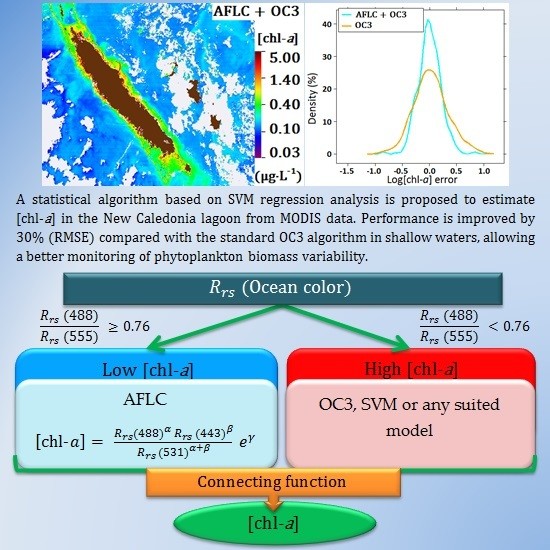
5. Conclusions

In this paper, we have introduced an algorithm for estimating [chl-a] from satellite-derived R_rs without a priori information, based solely on statistical considerations. Through this approach, we have obtained a suitable algorithm for optically complex waters of New Caledonia. The bottom influence in the lagoon is smaller than with OC3. The main improvement is obtained for waters with [chl-a] less than 3 µg·L⁻¹, with a RMSE 30% lower in average than with OC3 in New Caledonian lagoon waters. We have also shown satisfactory results for both world data and New Caledonia data.

It is notable, but not surprising, that the best explanatory variables from the SVM regression analysis are R_rs corresponding to wavelengths of blue and green light. For the data sets considered, the best wavelengths are 443, 488, and 531 nm. To classify a pixel in the group of high or low [chl-a], it is sufficient to simply use a threshold in the ratio of R_rs in the blue (488 nm) and green (555 nm), here 0.76 to separate waters with [chl-a] below and above 3 µg·L⁻¹. This algorithm is sensor-dependent but it had been constructed and checked with around 1400 match-ups from two different data sources. The risks of overtraining are very low and it is therefore possible to apply this algorithm at least to MODIS data. Tests should be performed to extend this algorithm to other sensors and coefficients should be adjusted accordingly.

A great deal of work is ongoing concerning atmospheric correction in coastal, optically complex waters. This is essential to obtain satisfactory match-ups. A major step will be made when much better agreement is obtained with in situ R_rs measurements. The [chl-a] algorithms will then provide more accurate results, allowing more efficient evaluation of the impact of environmental stress factors on lagoon ecosystems, especially coral reefs. Stress factors affect coral health both with intensity and time, hence the interest in having a continuous monitoring of water properties over large areas, which is only possible thanks to satellite data.