Article

Prediction of Soil Moisture Content and Soil Salt Concentration from Hyperspectral Laboratory and Field Data

1
State Key Laboratory of Water Resources and Hydropower Engineering Science, Wuhan University, Wuhan 430072, China
2
School of Natural Resources and the Environment, University of Arizona, Tucson, AZ 85721, USA
*
Author to whom correspondence should be addressed.
Remote Sens. 2016, 8(1), 42; https://doi.org/10.3390/rs8010042
Submission received: 25 November 2015 / Revised: 29 December 2015 / Accepted: 4 January 2016 / Published: 7 January 2016

Abstract

:
This research examines the simultaneous retrieval of surface soil moisture and salt concentrations using hyperspectral reflectance data in an arid environment. We conducted laboratory and outdoor field experiments in which we examined three key soil variables: soil moisture, salt and texture (silty loam, clay and silty clay). The soil moisture content models for multiple textures (M_SMC models) were based on selected hyperspectral reflectance data located around 1460, 1900 and 2010 nm and resulted in R2 values higher than 0.933. Meanwhile, the soil salt concentrations were also accurately (R2 > 0.748) modeled (M_SSC models) based on wavebands located at 540, 1740, 2010 and 2350 nm. When the different texture samples were mixed (SL + C + SC models), soil moisture was still accurately retrieved (R2 = 0.937) but the soil salt not as well (R2 = 0.47). After stratifying the samples by retrieved soil moisture levels, the R2 of calibrated M_SSCSMC models for soil salt concentrations improved to 0.951. This two-step method also showed applicability for analyzing soil-salt samples in the field. The M_SSCSMC models resulted in R2 values equal to 0.912 when moisture is lower than 0.15, and R2 values equal to 0.481 when soil moisture is between 0.15 and 0.2.

Graphical Abstract

1. Introduction

An irrigation monitoring program is often required to maintain soil moisture at a reasonable range to grow crops while reducing salinity risks and ecological concerns. Remote sensing technology is a tool that can provide geospatially extensive irrigation monitoring capabilities. Identification and monitoring of Soil Moisture Content (SMC) and Soil Salt Concentration (SSC) are important for setting up a sustainable and economically beneficial irrigation program. Precise and accurate measurements of SMC and SSC can be performed in a laboratory. One robust SMC indicator is gravimetric water content (GWC) [1], but it is restricted to a small volume of soil. For SSC measurements, electrical conductivity (EC), total soluble salts (TSS) [2], sodium adsorption ratio (SAR) and exchangeable sodium percentage (ESP) [3] are typical indicators. Some more practical in situ measurements of SMC and SSC, such as time domain reflectometry (TDR), electromagnetic induction, e.g., EM38 [4], Hydra-probe [5] and SCT-10, employ probes or sensors.
Remote sensing technology has the potential to measure soil moisture content (SMC) and soil salt concentration (SSC) across wide swaths in a nondestructive manner with a high temporal sampling frequency. Currently, there are three main remote sensing band widths applied to SMC and SSC monitoring: thermal infrared, microwave and optical (visible/near infrared/short wave infrared) electromagnetic radiation. Land surface temperature monitored via thermal infrared (TIR) energy (surface flux) is related to SMC conditions [6]. Coarse resolution SMC can be derived using the Atmosphere Land Exchange Inverse (ALEXI) model [7]. TIR regions are sensitive to salt emissivity properties and have been used to study SSC [8]. Microwave (MW) radiometers are suitable for predicting SMC and SSC even in non-precipitating cloudy weather conditions because of the large contrast between the dielectric properties of dry soil and water that result in variable microwave emissivity responses [9]. The C-band (5.3 GHz) and L-band (1.44 GHz) have shown promising results for SSC detection [10]. Nevertheless TIR and MW techniques often have the disadvantage of coarser sensor spatial resolutions (i.e., pixel size), because the footprint size often increases with increasing wavelength and decreasing signal levels. Passive optical remote sensing uses solar radiation as its energy source. The optical signature is directly related to surface properties, and quickly attenuates with soil depth. During the last few decades, much work has been done to characterize soil properties using optical spectral signatures that are mainly governed by absorption and reflectance. Quantities and mineralogy of salts, moisture content, color, and surface roughness [10,11,12] determine spectral reflectance data acquired by spectroradiometers and allow for SMC or SSC estimation [13,14,15,16].
Generally, the radiation reflected from soil surfaces varies with changes in soil constituents and wavelengths [17]. Most of the soil spectral variations occur in narrow wavelength regions that gradually fade with coarser bandwidths, or a limited number of spectral bands [18]. Nevertheless, conventional remote sensing data are commonly acquired by broad-band sensors such as Landsat TM or SPOT which have limited capacity to assess drought or saline affected areas.
Hyperspectral remote sensing can capture subtle differences in spectral soil properties. For example, Hyperion is a satellite based hyperspectral imager providing reflectance data at 10 nm bandwidths from 400 nm to 2500 nm. The ground-based Analytical Spectral Device (ASD) spectrometer (350–2500 nm) has the advantage of 1 nm spectral resolution. Hyperspectral data have great potential to quantify SMC and SSC because the hydrogen bond with soil water and soil salt concentrations result in subtle spectral changes [19]. Consequently, all the electronic processes and photon vibrational processes in response to overtones and combinations of minerals, water, and carbonates among others, are significant for the analysis of saline-soil using hyperspectral data. This is encouraging for monitoring SMC and SSC in arid or semi-arid lands [20]. Metternicht and Zinck [16] discussed the potential and constraints of salinity identification by remote sensing techniques, including hyperspectral technology. Ben-Dor, et al. [21] successfully applied a Visible and Near Infrared Analysis (VNIRA) approach to retrieve field soil moisture and salinity separately by using the hyperspectral airborne sensor DAIS–7915. Weng, et al. [22] calibrated a salinity index based on 2052 nm and 2203 nm bands with the ASD spectrometer (350–2500 nm), and evaluated its feasibility using the Hyperion reflectance image which resulted in R2 value of 0.627 [23]. Nawar, et al. [24] applied partial least squares regression (PLSR) and multivariate adaptive regression splines (MARS) to calibrate SSC models (R2 ≥ 0.87). Haubrock, et al. [25] developed a surface soil moisture model by using a soil moisture index (NSMI) resulting in a soil moisture map with R2 values of 0.82. Oltra-Carrió, et al. [26] further examined NSMI using laboratory and in situ data, and achieved R2 values larger than 0.76.
However, some weaknesses have been identified that limit SMC and SSC characterizations, especially in the field. First, most relations between reflectance measurements and salinity work best for severely salt-affected soils, but are weaker for slightly and moderately salt-affected areas [20]. The latter is the main challenge for salinity identification [27]. For cultivated farmland in arid and semi-arid areas, the magnitude of salinity often remains relatively low. Secondly, reflectance measurements are usually affected by soil texture [28], producing uncertainties in specific moisture or salt content assessments. Thirdly, both salt and moisture content could potentially result in similar soil reflectance or albedo data. In addition, increased moisture reduces albedo in a non-linear manner, and reduces the absorption features of the salty minerals [29,30]. Generally, soil salinity is hard to assess in wet soils.
The main objectives of this research are to: (1) examine the effect of soil moisture, salt and texture on both laboratory and field based hyperspectral reflectance data; and (2) develop an improved spectral methodology to quantify low and medium level soil moisture and salt levels. We pose that the measured or simulated soil moisture will be a valuable parameter for improving the soil salinity model.

2. Materials and Methods

We analyzed hyperspectral data as a function of soil moisture, salinity and texture mixtures. After examining the response of the hyperspectral reflectance measurements to surface soil and different proportions and levels of soil moisture, salt and texture, the reflectance response variables were expanded with three other transformations of the original reflectance data. Subsequently, their eigenvectors were analyzed to select the wavebands that explained the most variance. We used soil moisture information to stratify the samples to help with the modeling of soil salt concentrations.

2.1. Soil Preparation

To relate soil reflectance data with soil moisture, salt and texture, we conducted the following experimental procedures on synthetic soil samples (Figure 1a):
(1)
Soils were gathered from three study sites. Two of them are located in the Hetao Irrigation District, Inner Mongolia, China (108.01°E, 41.07°N), while the other one is located in Changzhou, China (119.97°E, 31.81°N).
(2)
Sand, silt, and clay proportions of the collected soil samples were quantified using the pipette method [31]. Results exhibited three textures: silty loam (SL, collected in Changzhou), clay and silty clay (C and SC, both were collected in the Hetao Irrigation District).
(3)
Salt from these soils were washed out and the soils air dried.
(4)
Salts were mixed using MgCl2, CaCl2, Na2CO3, NaHCO3, and Na2SO4 with molar concentration ratios of 11.74:8.54:1.00:15.39:20.83. These represent the average salt constitution in the Hetao Irrigation District.
(5)
Salty water solutions were made by mixing salt in certain amounts of water. We added these solutions to the air-dried soil to maintain the initial gravimetric soil moisture close to 0.3. Meanwhile, the nine different salt concentrations (g/g) were controlled to range from 0.1% to 1% (Table 1).
(6)
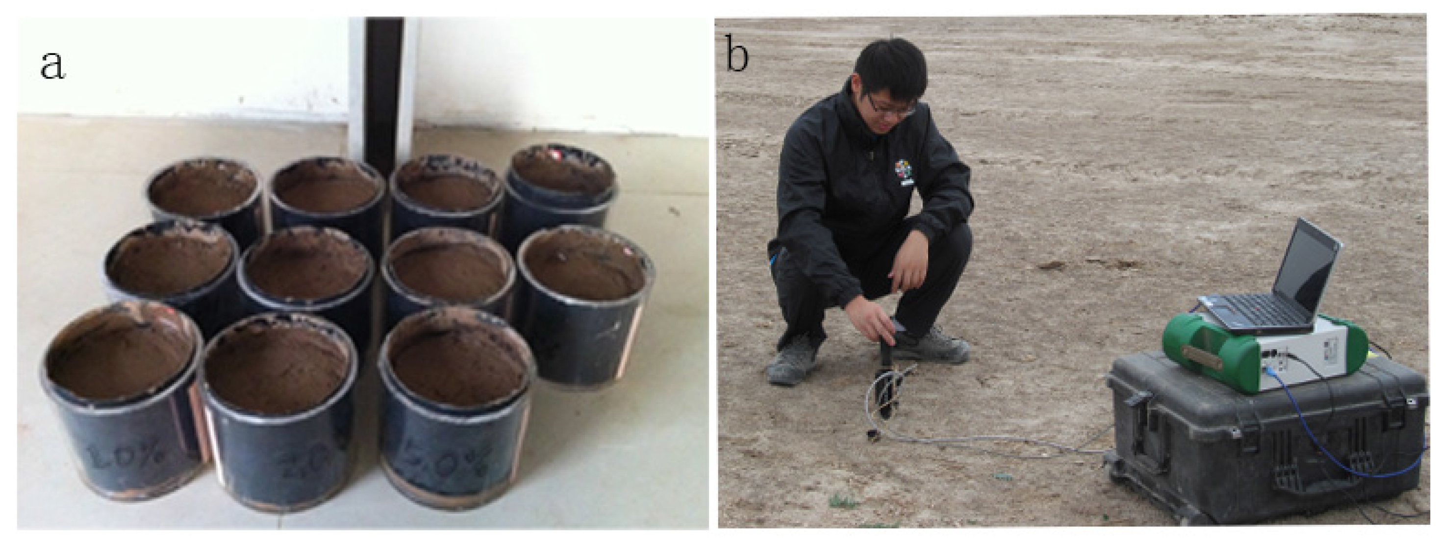
We filled the cylindrical container with soil and aimed (20 cm height and 15 cm diameter) to keep the soil bulk density at 1.4 g/cm3.
(7)
Time-series of surface hyperspectral reflectance data were measured while measuring the weight for these containers. Measurements continued until the container weights became constant. In total, there were nine measurements for the silty loam, ten measurements for clay and twelve measurements for silty clay.

2.2. Hyperspectral Measurements

We used the Analytical Spectral Device (ASD) AgriSpec (ASD, USA) spectrometer covering wavelengths from 400 to 2500 nm at an interval of one nm for spectral reflectance measurements. Soils were scanned with an ASD contact probe connected to the AgriSpec with a fiber-optic cable, having a 2 cm diameter circular viewing area and built-in halogen light source [32]. Relative reflectance is the quantity actually measured by the instrument, which is computed by dividing the energy reflected from the soil sample by the energy reflected off a calibrated white spectralon panel. The contact probe had full perpendicular contact with the soil surface. Twenty-five repetitive readings were averaged for each soil sample in order to minimize random noise. The dark current was also taken into account.

2.2.1. Laboratory Measurements

We conducted laboratory experiments by simultaneously weighing containers and measuring hyperspectral data for three sets of soil samples (SL, C and SC) during a two to four week period, depending on the decline of soil moisture in the containers (Table 1). To be more specific, the evaporation rate is mainly controlled by ambient conditions and soil texture. We paid close attention to the soil moisture content during the hyperspectral measurements. Each consecutive hyperspectral measurement was made after soil moisture changed between about 0.005 g/g and 0.05 g/g. The measurements and procedures for each group of soil texture samples lasted two to four weeks during which the soils dried out. Consequently, we measured hyperspectral soil reflectance values for different values and ratios of soil moisture, salinity and texture.
Table 1. Soil moisture, salt and texture characteristics of synthetic laboratory and field soil samples. (S.D. = standard deviation)
Laboratory Samples
Sampling SiteMoisture (g/g)Salt (g/g)Soil Texture
MinimumMaximumS.D.
Changzhou0.0400.2500.0580.1,0.2,0.3,0.4,0.5,0.6,0.7,0.8,1.0 (%)silty loam (SL)
Inner Mongolia0.0320.3520.0960.1,0.2,0.3,0.4,0.5,0.6,0.7,0.8,1.0 (%)Clay (C )
Inner Mongolia0.0530.3640.0950.1,0.15,0.2,0.3,0.4,0.5,0.6,0.7,0.8,1.0 (%)silty clay (SC)
Field Samples
Sampling SiteMoisture (g/g)Salt (g/g)
MinimumMaximumS.D.MinimumMaximumS.D.
Field0.1320.2380.0230.060%0.930%0.180%

2.2.2. Field Measurements

We conducted field experiments in Inner Mongolia, China in April of 2013 (Figure 1b). A total of 212 topsoil samples (up to a depth < 5 cm) were collected for analysis of soil and salt properties after in situ field spectral measurements were made using an ASD. The soil samples were measured for gravimetric soil moisture content (g/g) and soil salt concentration (g/g).
In the following content, SL, C, and SC are referring to the lab samples with soil texture of silty loam, clay and silty clay, respectively; ”SL + C + SC“ represents all three of the texture lab samples together; “Field” is specified for the field samples which have several soil textures including silty loam, clay, silty clay, silty clay loam, loam, silt, and clay loam.
Figure 1. (a) Prepared soil samples for laboratory measurements and (b) in situ field experiment using the Analytical Spectral Device (ASD) AgriSpec (ASD, USA) spectrometer.
Remotesensing 08 00042 g001

2.3. Spectral Transforms

After the soil surface hyperspectral reflectance values were measured by the ASD instrument, two spectral ranges, 350–400 nm and 2450–2500 nm, were discarded due to their low signal-to-noise ratio [29]. The retained 400–2450 nm reflectance values with one nm spectral resolution were converted to 10 nm by averaging every contiguous ten reflectance values. The majority of information was retained after these conversions. In addition, the 10 nm spectral resolution is consistent with the EO–1 Hyperion sensor [22].
It is difficult to extract a specific spectral signal solely from reflectance spectra (R) [33]. Consequently, we applied three other manipulations to the reflectance spectra to enhance the spectral information. The first spectral manipulation was the normalization (N) of reflectance spectra by the highest reflectance in that spectrum, which reduced the variation due to the intrinsic reflectance values of a soil [15]; the second and third spectral manipulations were the first (A′) and second derivative (A″) of apparent absorption (A) [A = log(1/R)] [33]. Consequently, reflectance (R), normalized reflectance spectra (N), first derivative (A′) and second derivative (A″) of apparent absorption were included in the modeling efforts (Figure 2). In order to standardize the scales of A′ and A″, we first normalized them to zero mean and unit variance.
Figure 2. Mean hyperspectral reflectance values of (a) Reflectance (R); (b) Normalized Reflectance (N); (c) First Derivative of log(1/R) (A′) and (d) Second Derivative of log(1/R) (A″) for silty loam (blue), clay (red), silty clay (black) and Field samples (purple). Dash lines indicate positive or negative standard deviation values from the mean value. The hyperspectral data in figure c and d is standardized to unit variance.
Remotesensing 08 00042 g002

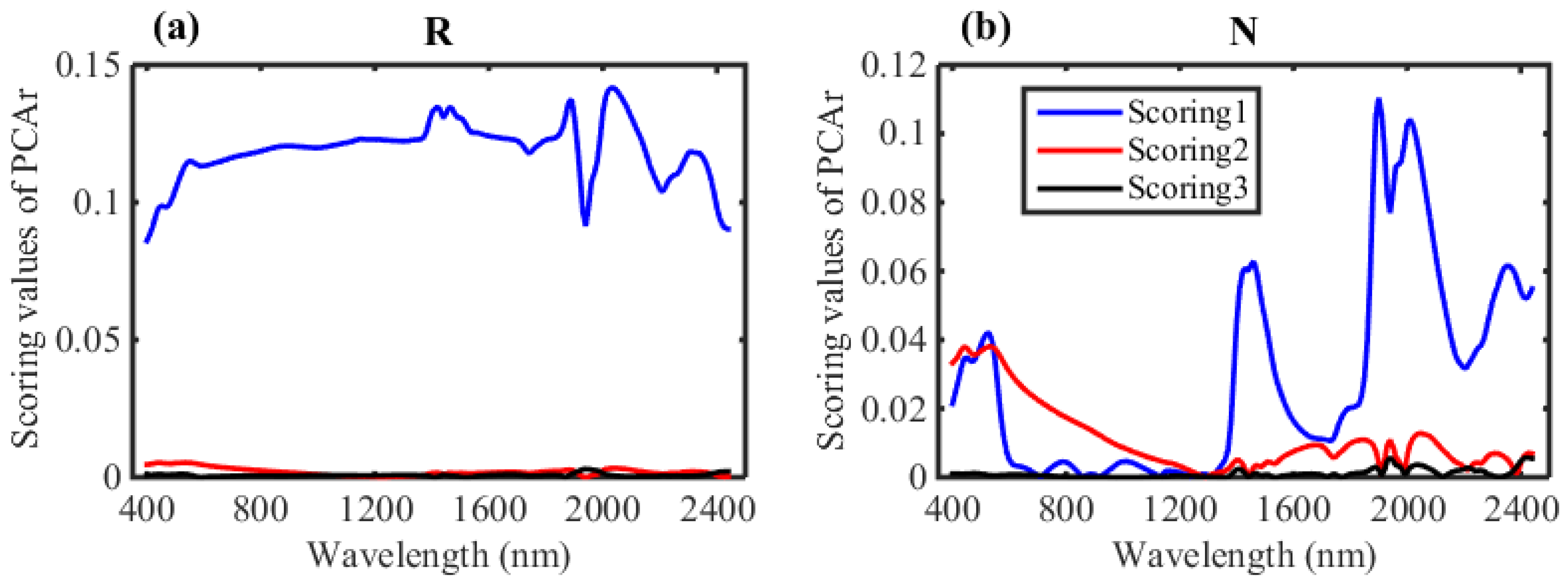
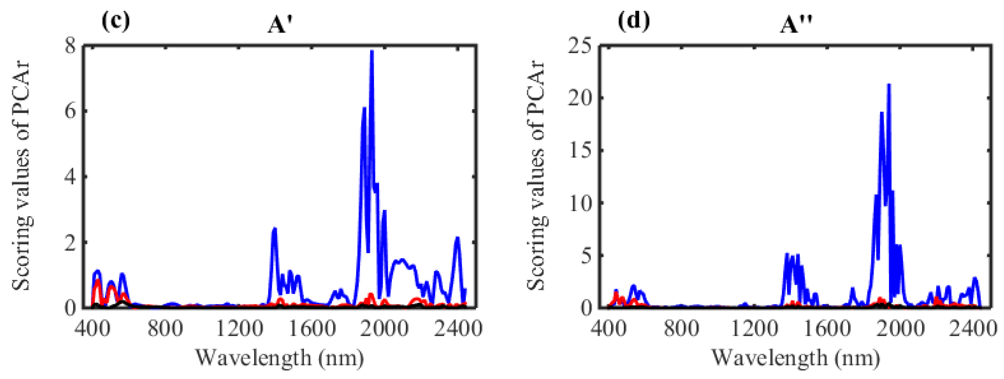
2.4. Waveband Selection of Sensitive Bands

According to William of Ockham, among competing hypotheses, the one with the fewest assumptions should be selected. To calibrate a parsimonious model, sensitive wavebands were selected according to the Principal Component Analysis (PCA) based ranking system (PCAr) [34]. PCA provides a multivariate overview to extract key variables that summarize and represent the variation in the hyperspectral reflectance signatures. The processes of PCA create two sets of outputs, the first are principal component coefficients (also known as loadings) and the second are principal component variances (also known as eigenvalues). The PCA based ranking system (PCAr) identifies the sensitive wavebands by the scoring values, which are the multiplication of the loadings and eigenvalues. Large scoring values for certain wavebands indicate the large contribution of these key variables.

2.5. Soil Moisture and Salt Model Calibration and Evaluation

We used a stepwise multiple linear regression [35] to relate reflectance to SMC and/or SSC. The p-values for each waveband we added to the model are 0.05 or smaller. After the predictors were selected by the scoring values of PCAr, stepwise regression analysis subsequently selected the most efficient predictors to build parsimonious M_SMC and M_SSC models. Since SMC is easier to interpret in salty wet soils than SSC, we also primarily derived SMCs from hyperspectral reflectance data, and subsequently used SMC as a parameter to enhance SSC inversion to build the M_SSCSMC model (Table 2).
We assessed both model calibration and evaluation for each dataset by separating the dataset into two groups by sorting them according to an ascending order of soil moisture content; then choosing the odd numbered samples for calibration, and using the rest of the samples for evaluation.
Table 2. Hyperspectral inversion models of soil moisture content and salt concentration.
Model NameFunctionInputs and Outputs
M_SMC SMC = f(Rλ, T)SMC—soil moisture content; SSC—soil salt concentration; Rλ or Nλ or Aλ′ or Aλ″—Spectral Reflectance & Transforms
T—exture
M_SSCSSC = f(Rλ, T)
M_SSCSMCSSC = f(Rλ, SMC)

2.6. Model Performance Indicators

Coefficient of determination (R2), relative Root Mean-Square Error (rRMSE) and Mean Error (ME) were the three statistical variables to test model performances. R2 values indicate how well the regression line approximates the measured data [36], rRMSE is the ratio between Root Mean-Square Error and the mean of the measured data, which indicates the relative estimated error [37]. The ME variable measures the bias between measured and predicted data.

3. Results and Discussion

3.1. Waveband Selections Sensitive to Soil Moisture and Salt

In order to calibrate and develop parsimonious models, a PCA based ranking system (PCAr) was applied to the SL + C + SC data set for R, N, A′ and A″. Sensitive wavebands were selected according to the scoring values of PCAr [34]. Specifically, most of the variance (sum of eigenvalues) was explained by the first three components (Figure 3) and was 99.8%, 98.5%, 95.1% and 90.5%, respectively for R, N, A′ and A″. The scoring values of the first principal component were larger than the second and third scoring values for the whole range of wavelengths. We thus mainly focused on the first scoring values of PCAr.
Figure 3. First three scoring values of hyperspectral reflectance variables: (a) Reflectance (R); (b) Normalized Reflectance (N); (c) First Derivative of log(1/R) (A′) and (d) Second Derivative of log(1/R) (A″) for SL + C + SC samples.
Remotesensing 08 00042 g003aRemotesensing 08 00042 g003b
The scoring value curves have clear patterns with some clear peaks, which are located in several sub-ranges: 400–600 nm, 1300–1550 nm, 1690–1800 nm, 1810–2200 nm and 2200–2450 nm (Figure 3). We subsequently refer to these spectral ranges as Zone 1, Zone 2, Zone 3, Zone 4 and Zone 5 here. Sensitive wavebands are selected for each zone based on simultaneous large first scoring values for R, N, A′ and A″. Finally, the fourteen selected wavebands (Table 3) represent the key bands that are sensitive to a range of different chemical and physical mechanisms. Each zone has a clear physical meaning in terms of photon absorption.
Table 3. Selected wavebands based on hyperspectral PCAr results along with reported corresponding active groups with physical mechanisms [38].
ZoneRangesSelected WavebandsPhysical MechanismActive Groups and Wavelength in Soil Spectrum
1400–600 nm440 nm, 540 nm, 570 nmCrystal-field effectsFe3+, Fe2+, Cr3+, Mn2+
Charge transferFe-O, B-O
21300–1550 nm1390 nm, 1430 nm, 1460 nmCrystal-field effectsFe2+, Ni2+
Vibrational processes2υ(OH-Al), 2υ32(H2O)
2υ(OH-Fe)
υ1+2υ3(H2O)
31690–1800 nm1740 nmCrystal-field effectsFe2+
Vibrational processes-
41810–2200 nm1870 nm, 1900 nm, 1940 nm, 2010 nmCrystal-field effectsFe2+
Vibrational processes2υ+δ (OH-P)
υ1+3υ3 (CO3)
υ13(H2O)
1+3υ3 (CO3)
υ1+2υ3 (CO3)
1+2υ1(CO3)
υ+2δ (OH-P)
52200–2450 nm2270 nm, 2350 nm, 2410 nmCrystal-field effectsFe2+
Vibrational processesυ+δ (OH-Al)
υ+δ (OH-Fe)
υ3 (CO3)
υ+δ (OH-Mg)
υ+δ (OH-P)
υ(H2O)
υ1+2υ3 (CO3)
In the range of 400–600 nm (Zone 1), the main process is occupied by crystal-field effects of transitional metal ions such as Cr, Fe and Mn [38]. At the same time, some charge-transfer, or inter-element electron transition produced by Fe-O, or B-O pairs also has influence [38]. In addition, some periodic minerals in soil, such as sulphur and cinnabar, have “conduction” electrons that show well-defined absorptions. Apart from that, soil organic matter has spectral activity in this visible region. In the other four zones (1300–2450 nm), spectral chromophores, which are defined as a parameter or substance that affects the shape and nature of a soil spectrum, are mostly produced by clay minerals, carbonates, water and soil salinity. Clay minerals and especially the hydroxide group (OH) are associated with overtones and combinations of fundamental vibrations in the NIR-SWIR range. For a general representative clay mineral like Ca-montmorillonite, a 2:1 layer silicate with a calcium saturated interlayer, has OH groups that absorb at 1410 nm and 2206 nm, whereas adsorbed OH features of free water are found at 1456 nm, 1910 nm and 1978 nm [39]. Carbonate ions exhibit features of overtones or combinations of the internal vibration between 1600 nm and 2500 nm [38]. Liquid water has overtones or combination features occurring at 1875, 1454, 1380, 1135 and 942 nm [38]. The spectral signature of saline soils can be a result of the salt itself or some other chromophores. The latter is indirectly related to the presence of the salt, such as water molecules, organic matter or particle size distribution [40]. Actually, these assigned positions are not constant, because they change slightly with actual chemical composition and surface activity [39]. The most common active groups and mechanisms affecting the soil spectrum are summarized in Table 3.

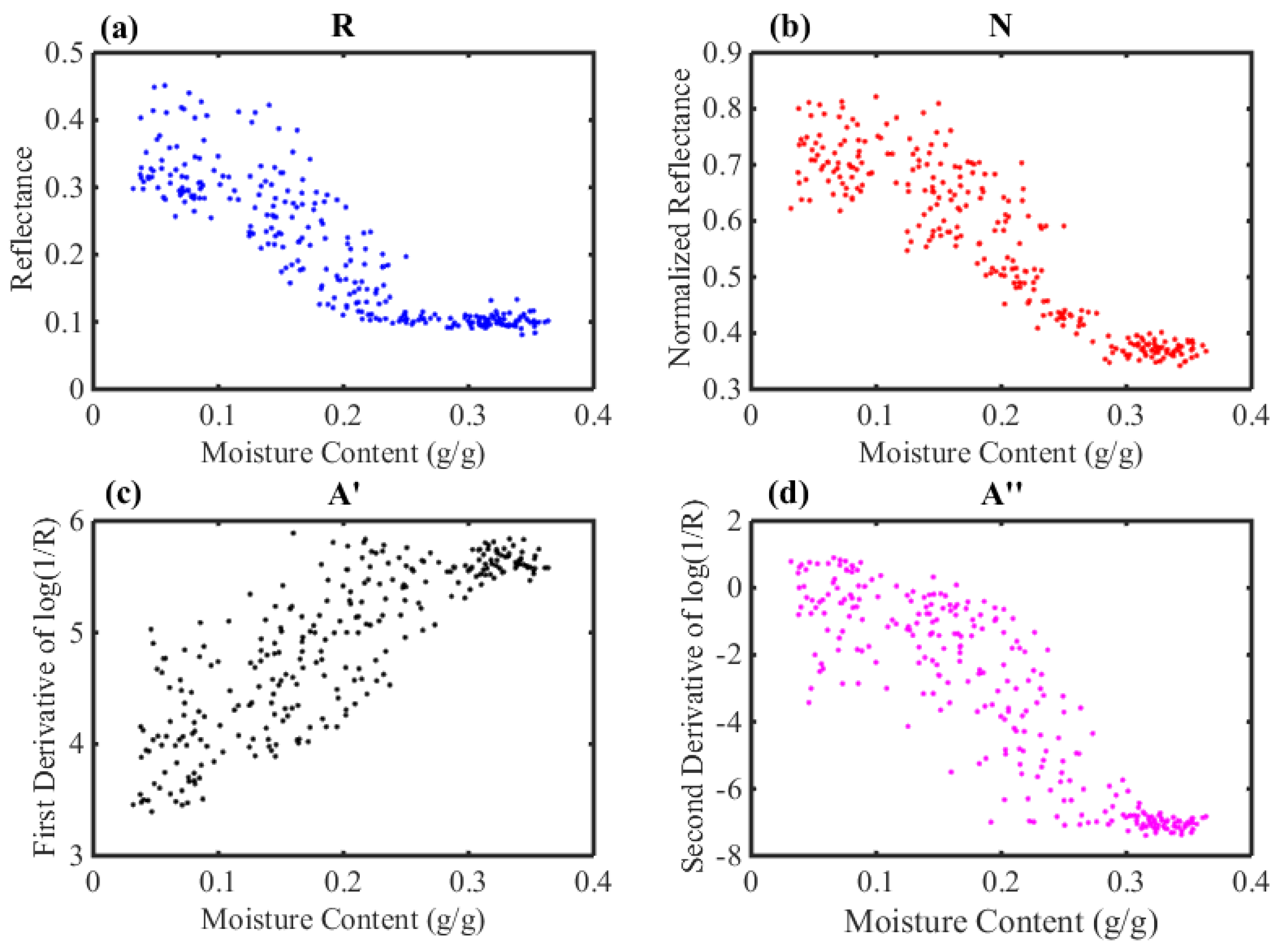
3.2. Soil Moisture Characterization

3.2.1. Relationship between Hyperspectral Reflectance and Soil Moisture

To discover the influence of moisture on hyperspectral reflectance values, we examined reflectance variations affected by various moisture contents for all selected wavebands (Figure 4, we only selected 1900 nm as a representative waveband). An obvious inflection point is always located around 0.3 gravimetric moisture content. R, N and A″ decrease as moisture increases from 0 to 0.3 SMC, while above 0.3 SMC, these variables do not change much. A′ increases with SMC as more radiation gets absorbed by soil moisture. In addition, for most arid and semi-arid farmland soil, the moisture content is generally lower than 0.3, hence we only examined the soil samples with moisture levels lower than 0.3 in the remaining presentation of the results and discussion.
Figure 4. Reflectance for wavelength of 1900 nm of (a) Reflectance (R); (b) Normalized Reflectance (N); (c) First Derivative of log(1/R) (A′) and (d) Second Derivative of log(1/R) (A″) with increasing soil moisture content for SL + C + SC samples.
Remotesensing 08 00042 g004

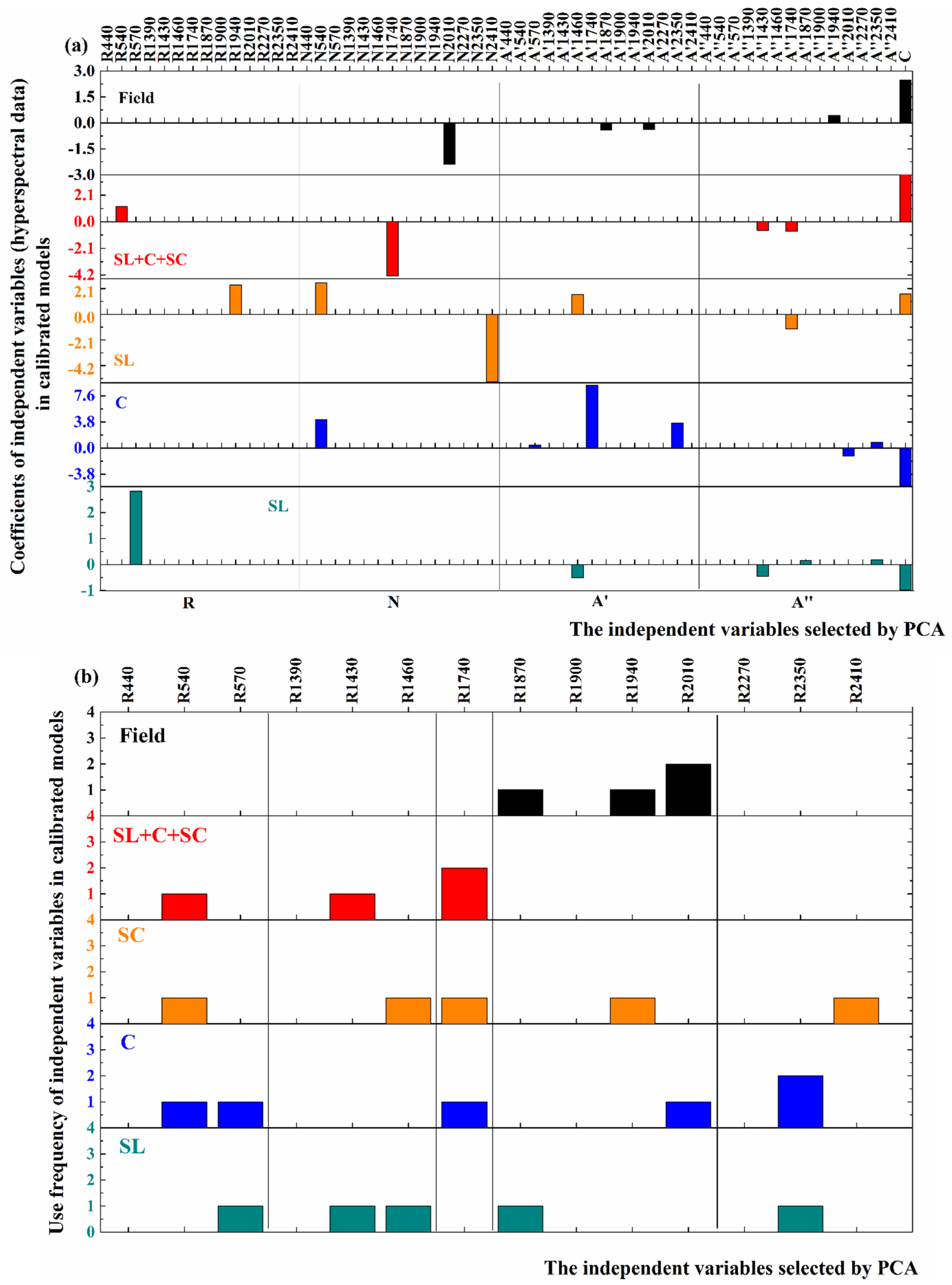
3.2.2. Calibration and Evaluation of M_SMC Models (SMC = f(Rλ, T)) for Soil Moisture Content

We used multi-linear stepwise regression for calibration and evaluation of the M_SMC models with the SL, S, SC, SL + C + SC and “Field” datasets. Generally, two to eight independent variables were selected to build these models. The statistical results showed that the (Table 4), SL, C, SC and SL + C + SC samples exhibit excellent fitting accuracy with small rRMSE (<0.115) for the model calibration, and also preserve very low rRMSE for the model evaluation with the independent data. The R2 is close to 1, which shows that the variance of measured soil moisture is modeled very well. This suggests that hyperspectral signatures can accurately derive SMC. Some uncertainty in the soil moisture quantification is attributed to soil texture (see M_SMC model for SL + C + SC) and salinity. Although the M_SMC model run with “Field” data also maintains the low fitting error (rRMSE = 0.085 for calibration, and rRMSE = 0.104 for evaluation), it does not simulate the measured soil moisture variance as well since the coefficient of determination (R2) is 0.529 for the calibrated model. Some of the reasons could be related to organic matter and soil porosity in the field [16]. All these calibrated and evaluated M_SMC models provide un-biased soil moisture estimates, since the mean error for all models is close to zero (i.e., ME Table 4). Among the five M_SMC models, the C model appears to be statistically the best, followed by the SC model. Meanwhile, it is also the most parsimonious model with just two independent variables.
Table 4. Statistical results for the calibration and evaluation of multi-textured soil moisture content models (M_SMC). The number of samples is shown for each calibration dataset. The evaluation dataset has the same number of samples or one less. The number of variables are indicated for each of the stepwise regression equations. Not included is the constant term.
Data setLabField
SLCSCSL + C + SC
Number of samples413533109106
Number of variables82684
CalibrationR20.9330.9730.9790.9370.529
rRMSE0.1150.0790.0610.1150.085
ME0.0000.0000.0000.0000.000
EvaluationR20.7580.9400.9130.8420.309
rRMSE0.2130.1170.1210.1810.104
ME0.001−0.002−0.0010.000−0.001
When comparing the coefficients of the independent variables of the M_SMC models (Figure 5a), the transformed hyperspectral data (N, A′ and A″) emerges more frequently than the reflectance data(R), especially for the “Field” model and SL + C + SC model, where none of the independent response variables is spectral reflectance. In addition, for the SC model and SL model, just one independent reflectance variable is selected, which is R440 for the SL model and R2410 for the SC model. These findings support the advantages of transforming the original reflectance data to bring out some subtle signature differences contained in the intrinsic hyperspectral reflectance data (N), A′ and A″. However, reflectance data of just two wavebands are enough to calibrate a precise model (C model) for clay data, which further illustrates that clay texture samples provide for easier retrieval of soil moisture.
Some of the selected wavebands exhibit auto-correlation, the wavebands extracted by the stepwise selection criteria [41] for model calibration are not consistent for the five M_SMC models.
Figure 5. Bar graphs for (a) coefficients of M_SMC models for soil moisture content, where C (last variable on the X-axis in (a) is a constant in the models; and (b) use frequency of the coefficients in different zone.
Remotesensing 08 00042 g005
Nevertheless, all the selected wavebands are related to water molecules and hydroxyl spectral interactions. Among the fourteen wavebands, ten of them: 440, 570, 1430, 1740, 1870, 1900, 2010, 2270, 2350 and 2410 nm appear in these models (Figure 5b), among which, 440 (visible range), 1430, 1900, 2010, 2270 and 2350 are (SWIR range) selected as independent variables more than three times. This implies that the SWIR range is significant for moisture identification. Similarly, Ben-Dor, et al. [42] suggested 2362 and 2120 nm are useful for prediction of arid and semiarid hygroscopic moisture; Dalal and Henry [43] recommended 1926, 1954 and 2150 nm for hygroscopic moisture estimation; Tian and Philpot [44] suggested that the spectral absorption features at 1440 and 1930 nm were strongly related to SMC during an entire drying period. These wavebands have clear physical mechanisms. For example, moisture absorption features located at 440 and 570 nm are possibly caused by the lattice water of minerals, such as chrysocolla and almandine. 1430 and 1900 nm have very strong absorption features (2υ1 + υ3 and υ2 + υ3) due to the vibrational process introduced by overtones and combinations by the fundamental vibrational modes. The other three sensitive wavebands, 2010, 2270 and 2350 nm are related with the hydroxyl (−OH) group, which are usually attached to Mg and Al, and produced the first overtone of the OH stretch near 1400 nm (the fundamental OH-stretching mode lie outside the SWIR range), or other bands in the 2000 nm region. The hygroscopic moisture (lattice water) attached in gypsum also displays some absorption features near these wavebands (See Table 3).
In order to build a more consistent and parsimonious model across all response variables, just one variable is selected for each of the hyperspectral R, N, A′ and A″ data transforms. Finally, four variables are chosen as the independent variables. Multi-linear regression is applied to calibrate the model. In total there are 144 kinds of possibilities for selecting independent variables, but the best prediction model, which has the largest sum of R2 for the five models of SL, C, SC, SL + C + SC and Field, is retained. In these simple consistent models, the combination of 1460, 1900 and 2010 nm is the best set of independent variables that make the best predictable model. Due to the high correlation between 1430 and 1460 nm, either one can represent the relative absorption features mentioned above. The simple models further demonstrate that the wavebands near 1400, 1900 and 2000 nm are sensitive to soil moisture.

3.3. Soil Salt Characterization

3.3.1. Calibration and Evaluation of Soil Salt Concentration Models (SSC = f(Rλ, T))

Four to six independent variables were chosen by the stepwise significance criteria, upon which soil salt inversion models (M_SSC) were established (Table 5). For the SSC models with three different soil textures, the SL SSC model explains the largest proportion of variance in soil salt that is estimated by the hyperspectral data (R2 = 0.874 for calibration, R2 = 0.730 for evaluation). The SC model is second best, with R2 = 0.822 for the model calibration, and R2 = 0.639 for the model evaluation. The C model has the lowest explained variation for the calibration (R2 = 0.748) and in particular for the evaluation (R2 = 0.282) model results. This implies that clay reduces the accuracy of the SSC inversion, while the silt component has less of an impact. The SSC is harder to predict when the three textures of the soil samples were mixed together in the SL + C + SC model (R2 = 0.47, rRMSE = 0.380), and confirms that soil texture is another important factor that influences the SSC inversion [45]. When we applied the M_SSC model to the field samples, the results did not compare well with the laboratory results. The evaluation of the calibrated M_SSC models shows some biases (i.e., ME Table 5) that are not observed in the M_SMC models (i.e., ME Table 4). Consequently, soil salt models are susceptible to soil texture and moisture and are therefore harder to develop compared to soil moisture models. This is especially true for arid-land field samples in our study area (R2 = 0.333, rRMSE = 0.526), where most areas maintain slight to moderate level soil salinity conditions [27].
Table 5. Statistics for calibration and evaluation of the soil salt concentration models (M_SSC). The number of samples is shown for each calibration dataset. The Evaluation dataset has the same number of samples or one less. The number of variables are indicated for each of the stepwise regression equations. The constant term is not included in this table.
Data setLabField
SLCSCSL + C + SC
Number of samples413533109106
Number of variables56544
CalibrationR20.8740.7480.8280.4700.333
rRMSE0.2060.2430.2000.3800.526
ME0.0000.0000.0000.0000.000
EvaluationR20.7300.2820.6390.5430.306
rRMSE0.3040.5300.3440.3680.529
ME−0.0900.016−0.006−0.026−0.020
When we compare the use frequency of the independent variables by the stepwise regression models, it is obvious that the N, A′ and A″ transforms appear more frequently than the reflectance (R) variables (Figure 6a). Among the five models, the “Field” model and C model do not select any reflectance bands as independent variables. Nevertheless, the hyperspectral manipulations, especially the A″ transform, which appears up to nine times in these five models, is always used as an independent variable. Therefore, including soil moisture conditions and transforms of the original hyperspectral data are important for optimizing soil salt retrievals.
Ten of the originally chosen fourteen wavebands, 540, 570, 1430, 1460, 1740, 1870, 1940, 2010, 2350 and 2410 nm are selected as significant (p ≤ 0.05) independent variables to model soil salt concentrations (Figure 6b). This also implies that these wavebands are related to the reflectance and absorption features of soil salt. Because some similar wavebands can be retrieved from the Advanced Land Imager (ALI) to make good quality (R2 > 0.689) soil salinity predictions [46], the calibrated models have good application prospects. Among the wavebands, 540, 1740, 2010 and 2350 nm appear more than three times as the independent variables in the stepwise regression models. These four regions have more intense electronic and vibrational processes directly connected with the spectral signature of salt, or indirectly connected with other chromophores, such as water, due to the presence of salt. The main cations and anions that constitute the soil salt of the study area are Mg, Ca, Na, and Cl, CO3, HCO3, respectively. These ions constitute some typical minerals which have characteristic absorption features. For example, Farifteh, et al. [47] reported that Bischofite (MgCl2∙6H2O) has absorption features located around 758, 985, 1190, 1451, 1556, 1824 and 1952 nm, similar to the 1451, 1824 and 1952 nm bands we identified.
Figure 6. Bar graphs for (a) coefficients of M_SSC models for soil salt concentration, where C (last variable on the X-axis in (a) is a constant in the models; and (b) use frequency of the independent variables/wavebands in the calibration models.
Remotesensing 08 00042 g006
We found a high correlation between similar wavebands at 1430, 1870 and 1940 nm. Halite (NaCl) has absorption features located at 1440 and 1933 nm, and Epsomite (MgSO4∙7H2O) has absorption features at 793, 999, 1240, 1490, 1631, 1760 and 1946 nm. This confirms that the wavebands that we used, 1430, 1740 and 1940 nm, were significant in retrieving Halite and Epsomite. Hunt [38] states that gypsum (CaSO4∙2H2O) has absorption features around 1000, 1200, 1400, 1700, 2000, 2200 and 2500 nm due to the presence of water at specific sites essential to the structure of the mineral. Carbonate (CaCO3) and Ca bicarbonate (CaHCO3) ions have overtones or combinations of the internal vibrations which produce absorption features between 1600 and 2500 nm, including 2350 nm (3υ3), 2160 nm (υ1 + 2υ3 + υ4 and 3υ1 + 2υ4), 2000 nm (2υ1 + 2υ3) and 1900 nm (υ1 + 3υ3) [38]. Actually, the spectral signals related to the given minerals overlap with each other, thereby obscuring the obvious absorption features solely attributable to one kind of mineral. As a result, the above presented absorption features can vary according to the actual natural situations and could be impacted by a variety of soil components such as mineral composition, moisture content and soil porosity. In our study, although we resampled the spectral resolution to 10 nm, the detected absorption features were similar as reported for finer spectral resolution data in the literature [38].

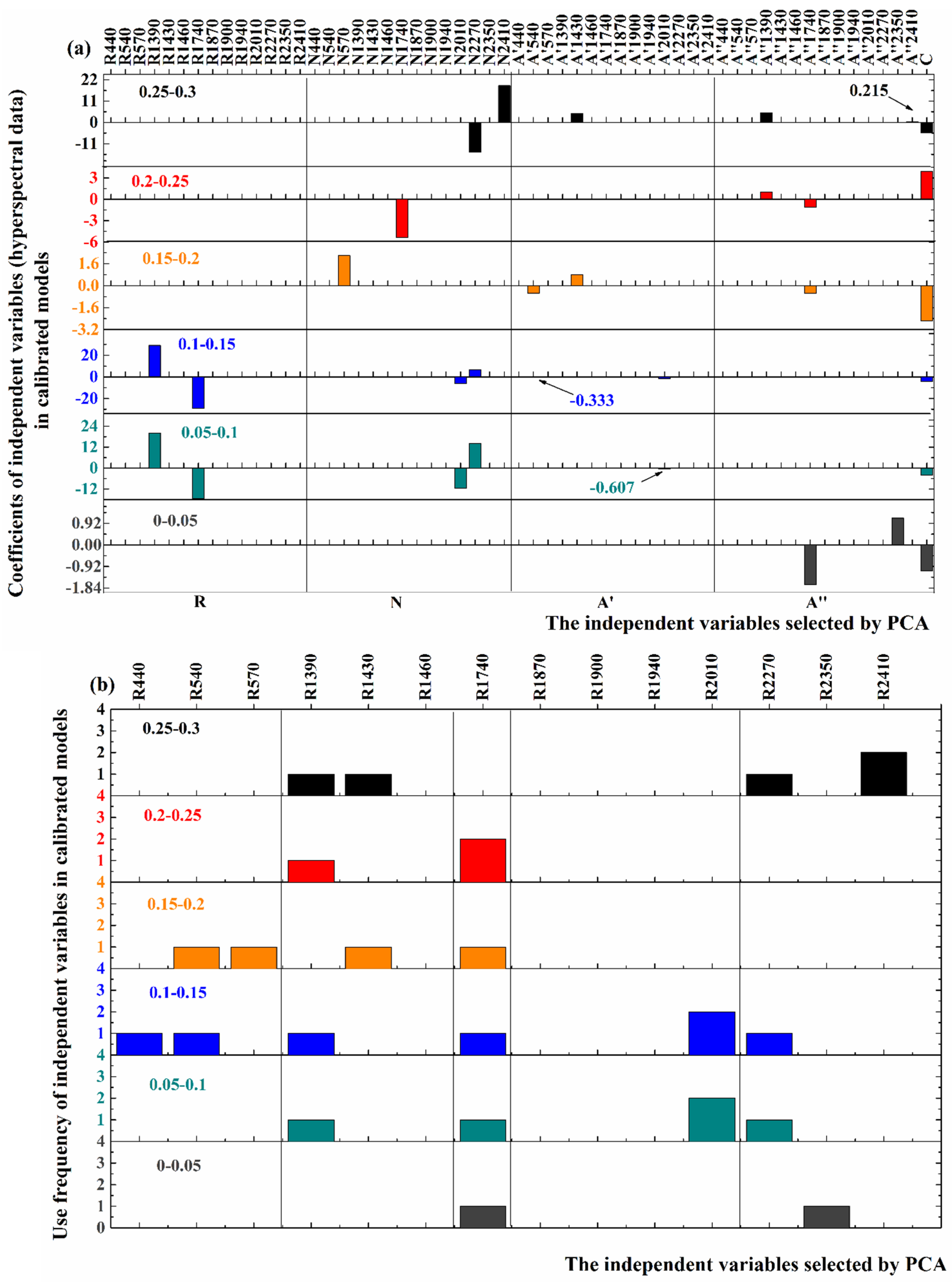
3.3.2. Calibration of M_SSCSMC Models (SSC = f(Rλ, SMC)) for Soil Salt Concentration

Because soil surface salinity is highly correlated with the hygroscopic soil moisture content, as was pointed out by Ben-Dor [48], the impact of soil moisture on the retrieval of soil salt concentrations was taken into account by separating soil samples into sub-samples according to predicted soil moisture levels (see Section 3.2.2.) M_SSCSMC models used to predict soil salt concentrations were calibrated using stepwise regression. The soil salt modeling results are displayed for 0.05 soil moisture intervals in Table 6.
Table 6. Statistics for calibration results of M_SSCSMC models for soil salt concentration. The number of samples is shown for each calibration dataset. The number of variables are indicated for each of the stepwise regression equations. Not included is the constant term.
SMC Scale0–0.050.05–0.10.1–0.150.15–0.20.2–0.250.25–0.3
SL + C + SCNumber of samples114454444416
Number of variables257435
R20.739 0.801 0.848 0.637 0.631 0.951
rRMSE0.366 0.251 0.201 0.294 0.293 0.132
ME0.000 0.000 0.000 0.000 0.000 0.000
FieldNumber of samples\716342\
Number of variables262
R20.912 0.481 0.316
rRMSE0.175 0.479 0.451
ME0.000 0.000 0.000
Due to the limited sample size, the M_SSCSMC models only include SL + C + SC laboratory samples, where all M_SSCSMC models represent compelling higher explained variance and a lower relative Root Mean-Square Error respectively (0.63 < R2 < 0.95, 0.132 < rRMSE < 0.366) than the previous M_SSC model (Table 5, R2 = 0.47, rRMSE = 0.380). More specifically, soil salinity was better predicted when the gravimetric moisture contents of the samples are lower than 0.15 or higher than 0.25 (Table 6). Moderate moisture values in the range of 0.15 to 0.25 were less predictable.
During the experiments, upward water and salt movement was due to evaporation. Therefore, the surface soil moisture was likely slightly smaller than the mean value of the containers. Over time some of the soil salt concentrations at the surface are likely slightly higher than the mean salt concentration of the container. Because we used the mean values in the containers, the continuous evaporation process likely overestimated actual surface soil moisture content and likely underestimated the actual salt concentration. Soil moisture content measured for the “Field” samples only ranged from 0.132 to 0.238. Therefore, three sub-groups were examined with a 0.05 moisture interval. Among the three sub-groups, only 7 samples were located in the moisture range of 0.1 to 0.15. The relative M_SSCSMC model shows good statistical results (R2 = 0.912, rRMSE = 0.175) when 2 independent variables are used for calibration. The sample quantity is the largest when moisture ranges from 0.15 to 0.2, and the regression results of this M_SSCSMC model are better than the M_SSC model (Table 5). The “Field” samples with moisture content from 0.2 to 0.25, exhibit statistics for the M_SSCSMC models (Table 6) almost equivalent to the M_SSC models (Table 5). Comparatively speaking, “Field” M_SSCSMC models do not provide much improvement in salinity retrieval in the moisture range of 0.15 to 0.25. We suggest that more in situ field experiments should be conducted with a wider range of moisture levels to further test the applicability of this approach. Meanwhile, we collected the top 5 cm of each soil sample and measured the mean soil moisture content and soil salt concentration. This likely introduces some uncertainties when establishing the hyperspectral inversion models, because the hyperspectral signatures are related directly to surface soil properties, rather than the mean value of the top 5 cm. We also suggest including organic matter levels along with soil moisture, salt and texture in the interaction analysis, because the spectral response of organic matter might have some responses similar to soil moisture.
The independent variable selection for the M_SSCSMC models (Figure 7a) is closely related with the moisture range. When soil moisture is lower than 0.05, only the second derivative of reflectance data at two wavebands, 1740 and 2350 nm, are selected as efficient independent variables in the stepwise regression model for inversion of salt concentrations (Figure 7a). When the soil moisture content is between 0.05 and 0.15, the reflectance at 1390 and 1740 nm, as well as normalized reflectance at 2010 and 2270 nm are the common independent variables. When soil moisture is greater than 0.15, the reflectance transforms N, A′ and A″ are kept as independent variables, while all original reflectance variables are not used.
Bands at 440, 540, 570, 1390, 1430, 1740, 2010, 2270, 2350 and 2410 nm are selected as independent variables in the M_SSCSMC models (Figure 7b). Four of them, 1390, 1740, 2010 and 2270 nm appear more frequently than other wavebands. Consequently, 1740 nm is the most important wavebands for calibrating the salt sub-model. The use frequency of certain wavebands in the M_SSCSMC models are a little different from M_SSC models (Figure 6b), and implies that this method calibrates the models more skillfully after the samples are grouped according to the retrieved soil moisture levels.
The coefficients for the “Field” M_SSCSMC models, show similar patterns as the SL + C + SC M_SSCSMC models. The reflectance transforms, especially the first and second derivative value, appear to be more significant in the regression models (Figure 8a) than the reflectance data. The stepwise regression selected wavebands at 440, 1390, 1430, 1740, 1870, 1900, 2010 and 2270 nm as significant independent variables (Figure 8b). Consequently, the developed models can be applied to multispectral missions such as Sentinel-2, which has medium spatial resolution (10–60 m) and 13 spectral bands. Sentinel-2 bands at 443, 490, 560,1375, 1610, 2190 nm are efficient bands that could be used as variables in our models [49]. Compared with traditional field sampling and chemical analysis, our models could be more economic and save time once calibrated and established. In addition, with the development of computing and remote sensing technology, the costs and time required for applying our models have become less expensive and more acceptable. These predictive SMC and SSC models can likely also be used for other soil properties such as soil organic carbon [50,51,52,53].
Figure 7. Bar graphs for (a) coefficients of laboratory SL + C + SC M_SSCSMC models for soil salt concentration (some coefficient values are too small to mark with bar plots, so values with arrows are plotted to identify them), where C (last variable on the X-axis in (a) is a constant in the models; and (b) use frequency of the coefficients/wavebands in different zones.
Remotesensing 08 00042 g007
Figure 8. Bar graphs for (a) coefficients of Field M_SSCSMC models for soil salt concentration (some coefficient values are too small to mark with bar plots, so values with arrows are plotted to identify them), where C (last variable on the X-axis in (a) is a constant in the models; and (b) use frequency of the salt model coefficients/wavebands for different soil moisture ranges.
Remotesensing 08 00042 g008

4. Conclusions

Inversion of soil moisture and salt concentration using remote sensed spectral technology is meaningful for agricultural management, especially in the vast arid and semi-arid lands [54] that encompass ~35% of the earth’s land surface. Nevertheless, moisture, salt and texture soil properties all simultaneously influence soil spectra [55], which makes single soil property inversions for soil moisture or salt concentration more complicated.
Our modeling results also show that the transforms of normalized reflectance (N), first derivative values (A′) and second derivative values (A″) of the absorption, can improve our soil moisture and salt modeling predictions. At the same time, hyperspectral waveband selections are crucial for developing soil moisture, salt and texture based models. The selected wavebands reduce the dimensionality and represent the variability in the spectral data sets, the development of simple soil moisture and salt models are feasible.
Our findings indicate that relative to soil salt, the soil moisture models are easier to interpret because they are less sensitive to soil salt and texture. On the other hand, soil salt models are more susceptible to soil moisture and texture. Consequently, we retrieved both soil moisture and salt simultaneously, by including the accurately estimated soil moisture (0.032–0.364 for laboratory samples, 0.132–0.238 for field samples) as a factor to separate samples into several sub-groups. Compared with the results from direct retrieval, soil salinity (0.1%–1.0% g/g for laboratory samples, and 0.06%–0.932% g/g for field samples) retrieval improves when soil moisture estimates are included in the models. Furthermore, our methodology also performs well for the field samples. We showed that the remote sensing methodologies coupled with reflectance spectroscopy techniques have the potential to provide non-destructive and rapid predictions of soil moisture and salt in the short-term at low cost and an acceptable level of error.

Acknowledgments

This research is supported by the State Natural Science Funds (Research on the Production Function of Water–fertilizer in Saline Soil Based on Crop Growth Simulation grant No. 51379151, and Soil Salinization Prediction of Irrigation District Based on Data Assimilation grant No. 51279142), China Postdoctoral Science Foundation (No. 2015M582274), and the Fundamental Research Funds for the Central Universities (grant No. 2014206020201).

Author Contributions

Chi Xu wrote the paper and did the experiments; Wenzhi Zeng, supervised the study, did part of the experiments, reviewed and edited the manuscript; Jiesheng Huang supervised the study and reviewed the manuscript; Jingwei Wu reviewed the manuscript; Willem J.D. van Leeuwen provided feedback to the research and helped with editing the manuscript. All authors read and approved the manuscript.

Conflicts of Interest

The authors declare no conflict of interest.

References

  1. Klute, A. Methods of Soil Analysis. Part 1. Physical and Mineralogical Methods; American Society of Agronomy, Inc.: Madison, WI, USA, 1986. [Google Scholar]
  2. Rhoades, J. Salinity: Electrical conductivity and total dissolved solids. Methods Soil Anal. Part 1996, 3, 417–435. [Google Scholar]
  3. Paliwal, K.; Gandhi, A. Effect of salinity, SAR, Ca: Mg Ratio in Irrigation Water, and Soil Texture on the Predictability of Exchangeable Sodium Percentage. Soil Sci. 1976, 122, 85–90. [Google Scholar] [CrossRef]
  4. Schelde, K.; Thomsen, A.; Hougaard, H. Comparison of EM38 and TDR measurements of soil moisture and electrical conductivity. In Proceedings of the 5th European Conference on Precision Agriculture, Uppsala, Sweden, 9–12 June 2005.
  5. Seyfried, M.; Grant, L.; Du, E.; Humes, K. Dielectric loss and calibration of the Hydra Probe soil water sensor. Vadose Zone J. 2005, 4, 1070–1079. [Google Scholar] [CrossRef]
  6. Anderson, M.C.; Norman, J.M.; Mecikalski, J.R.; Otkin, J.A.; Kustas, W.P. A climatological study of evapotranspiration and moisture stress across the continental united states based on thermal remote sensing: 1. Model formulation. J. Geophys. Res.: Atmos. 2007, 112, D10. [Google Scholar] [CrossRef]
  7. Hain, C.R.; Mecikalski, J.R.; Anderson, M.C. Retrieval of an available water-based soil moisture proxy from thermal infrared remote sensing. Part I: Methodology and validation. J. Hydrometeorol. 2009, 10, 665–683. [Google Scholar] [CrossRef]
  8. Lane, M. Upcoming Themis investigation of salts on Mars. In Proceedings of the Lunar and Planetary Science Conference, League City, TX, USA, 11–15 March 2002.
  9. Schmugge, T.; Gloersen, P.; Wilheit, T.; Geiger, F. Remote sensing of soil moisture with microwave radiometers. J. Geophys. Res. 1974, 79, 317–323. [Google Scholar] [CrossRef]
  10. Mougenot, B.; Pouget, M.; Epema, G.F. Remote sensing of salt affected soils. Remote Sens. Rev. 1993, 7, 241–259. [Google Scholar] [CrossRef]
  11. Ciani, A.; Goss, K.U.; Schwarzenbach, R.P. Light penetration in soil and particulate minerals. Eur. J. Soil Sci. 2005, 56, 561–574. [Google Scholar] [CrossRef]
  12. Skidmore, E.L.; Dickerson, J.D.; Schimmelpfennig, H. Evaluating surface-soil water content by measuring reflectance. Soil Sci. Soc. Am. J. 1975, 39, 238–242. [Google Scholar] [CrossRef]
  13. Ben-Dor, E.; Chabrillat, S.; Demattê, J.A.M.; Taylor, G.R.; Hill, J.; Whiting, M.L.; Sommer, S. Using imaging spectroscopy to study soil properties. Remote Sens. Environ. 2009, 113, S38–S55. [Google Scholar] [CrossRef]
  14. Van der Meer, F. Analysis of spectral absorption features in hyperspectral imagery. Int. J. Appl. Earth Obs. Geoinf. 2004, 5, 55–68. [Google Scholar] [CrossRef]
  15. Whiting, M.L.; Li, L.; Ustin, S.L. Predicting water content using gaussian model on soil spectra. Remote Sens. Environ. 2004, 89, 535–552. [Google Scholar] [CrossRef]
  16. Metternicht, G.I.; Zinck, J.A. Remote sensing of soil salinity: Potentials and constraints. Remote Sens. Environ. 2003, 85, 1–20. [Google Scholar] [CrossRef]
  17. Csillag, F.; Pásztor, L.; Biehl, L.L. Spectral band selection for the characterization of salinity status of soils. Remote Sens. Environ. 1993, 43, 231–242. [Google Scholar] [CrossRef]
  18. Cloutis, E. Review article hyperspectral geological remote sensing: Evaluation of analytical techniques. Int. J. Remote Sens. 1996, 17, 2215–2242. [Google Scholar] [CrossRef]
  19. Hirschfeld, T. Salinity determination using nira. Appl. Spectrosc. 1985, 39, 740–741. [Google Scholar] [CrossRef]
  20. Wang, Q.; Li, P.; Chen, X. Modeling salinity effects on soil reflectance under various moisture conditions and its inverse application: A laboratory experiment. Geoderma 2012, 170, 103–111. [Google Scholar] [CrossRef]
  21. Ben-Dor, E.; Patkin, K.; Banin, A.; Karnieli, A. Mapping of several soil properties using DAIS-7915 hyperspectral scanner data—A case study over clayey soils in Israel. Int. J. Remote Sens. 2002, 23, 1043–1062. [Google Scholar] [CrossRef]
  22. Weng, Y.; Gong, P.; Zhu, Z. Reflectance spectroscopy for the assessment of soil salt content in soils of the yellow river delta of China. Int. J. Remote Sens. 2008, 29, 5511–5531. [Google Scholar] [CrossRef]
  23. Weng, Y.L.; Gong, P.; Zhu, Z.L. A spectral index for estimating soil salinity in the yellow river delta region of china using eo-1 hyperion data. Pedosphere 2010, 20, 378–388. [Google Scholar] [CrossRef]
  24. Nawar, S.; Buddenbaum, H.; Hill, J.; Kozak, J. Modeling and mapping of soil salinity with reflectance spectroscopy and landsat data using two quantitative methods (PLSR and MARS). Remote Sens. 2014, 6, 10813–10834. [Google Scholar] [CrossRef]
  25. Haubrock, S.N.; Chabrillat, S.; Kuhnert, M.; Hostert, P.; Kaufmann, H. Surface soil moisture quantification and validation based on hyperspectral data and field measurements. J. Appl. Remote Sens. 2008, 2, 023552. [Google Scholar] [CrossRef]
  26. Oltra-Carrió, R.; Baup, F.; Fabre, S.; Fieuzal, R.; Briottet, X. Improvement of soil moisture retrieval from hyperspectral vnir-swir data using clay content information: From laboratory to field experiments. Remote Sens. 2015, 7, 3184–3205. [Google Scholar] [CrossRef]
  27. Farifteh, J.; Farshad, A.; George, R.J. Assessing salt-affected soils using remote sensing, solute modelling, and geophysics. Geoderma 2006, 130, 191–206. [Google Scholar] [CrossRef]
  28. Yao, Y.; Wei, N.; Chen, Y.; He, Y.; Tang, P. Soil moisture monitoring using hyper-spectral remote sensing technology. In Proceedings of the 2010 Second IITA International Conference on Geoscience and Remote Sensing (IITA-GRS), Qingdao, China, 28–31 August 2010; pp. 373–376.
  29. Weidong, L.; Baret, F.; Xingfa, G.; Qingxi, T.; Lanfen, Z.; Bing, Z. Relating soil surface moisture to reflectance. Remote Sens. Environ. 2002, 81, 238–246. [Google Scholar] [CrossRef]
  30. Whiting, M.L.; Ustin, S.L.; Zarco-Tejada, P.; Palacios-Orueta, A.; Vanderbilt, V.C. Hyperspectral mapping of crop and soils for precision agriculture. Proc. SPIE 2006, 6298, 62980B. [Google Scholar] [CrossRef]
  31. Miller, W.; Miller, D. A micro-pipette method for soil mechanical analysis. Commun. Soil Sci. Plant Anal. 1987, 18, 1–15. [Google Scholar] [CrossRef]
  32. Chakraborty, S.; Weindorf, D.C.; Ali, M.N.; Li, B.; Ge, Y.; Darilek, J.L. Spectral data mining for rapid measurement of organic matter in unsieved moist compost. Appl. Opt. 2013, 52, B82–B92. [Google Scholar] [CrossRef] [PubMed]
  33. Ben-Dor, E.; Inbar, Y.; Chen, Y. The reflectance spectra of organic matter in the visible near-infrared and short wave infrared region (400–2500 nm) during a controlled decomposition process. Remote Sens. Environ. 1997, 61, 1–15. [Google Scholar] [CrossRef]
  34. Bajcsy, P.; Groves, P. Methodology for hyperspectral band selection. Photogramm. Eng. Remote Sens. 2004, 70, 793–802. [Google Scholar] [CrossRef]
  35. Kokaly, R.F.; Clark, R.N. Spectroscopic determination of leaf biochemistry using band-depth analysis of absorption features and stepwise multiple linear regression. Remote Sens. Environ. 1999, 67, 267–287. [Google Scholar] [CrossRef]
  36. Mtamba, J.; van der Velde, R.; Ndomba, P.; Zoltán, V.; Mtalo, F. Use of Radarsat-2 and Landsat TM images for spatial parameterization of manning’s roughness coefficient in hydraulic modeling. Remote Sens. 2015, 7, 836–864. [Google Scholar] [CrossRef]
  37. Corona, P.; Fattorini, L.; Franceschi, S.; Chirici, G.; Maselli, F.; Secondi, L. Mapping by spatial predictors exploiting remotely sensed and ground data: A comparative design-based perspective. Remote Sens. Environ. 2014, 152, 29–37. [Google Scholar] [CrossRef] [Green Version]
  38. Hunt, G.R. Spectral signatures of particulate minerals in the visible and near infrared. Geophysics 1977, 42, 501–513. [Google Scholar] [CrossRef] [Green Version]
  39. Ryerson, R. Manual of Remote Sensing, Volume 3: Remote Sensing for the Earth Sciences; American Society for Photogrammetry and Remote Sensing, John Wiley & Sons: New York, NY, USA, 1999. [Google Scholar]
  40. Hick, P.; Russell, W. Some spectral considerations for remote sensing of soil salinity. Soil Res. 1990, 28, 417–431. [Google Scholar] [CrossRef]
  41. Derksen, S.; Keselman, H. Backward, forward and stepwise automated subset selection algorithms: Frequency of obtaining authentic and noise variables. Br. J. Math. Stat. Psychol. 1992, 45, 265–282. [Google Scholar] [CrossRef]
  42. Ben-Dor, E.; Banin, A.; Singer, A. Simultaneous determination of six important soil properties by diffuse reflectance in the near infrared region. In Proceedings of the 5th International Colloquium on Physical Measures and Signatures in Remote Sensing, Courchevel, France, 14–18 January 1991; pp. 159–163.
  43. Dalal, R.; Henry, R. Simultaneous determination of moisture, organic carbon, and total nitrogen by near infrared reflectance spectrophotometry. Soil Sci. Soc. Am. J. 1986, 50, 120–123. [Google Scholar] [CrossRef]
  44. Tian, J.; Philpot, W.D. Relationship between surface soil water content, evaporation rate, and water absorption band depths in swir reflectance spectra. Remote Sens. Environ. 2015, 169, 280–289. [Google Scholar] [CrossRef]
  45. Metternicht, G.; Zinck, A. Remote Sensing of Soil Salinization: Impact on Land Management; CRC Press: Boca Raton, FL, USA, 2008. [Google Scholar]
  46. Fan, X.; Liu, Y.; Tao, J.; Weng, Y. Soil salinity retrieval from advanced multi-spectral sensor with Partial Least Square Regression. Remote Sens. 2015, 7, 488–511. [Google Scholar] [CrossRef]
  47. Farifteh, J.; Tolpekin, V.; van der Meer, F.; Sukchan, S. Salinity modelling by inverted gaussian parameters of soil reflectance spectra. Int. J. Remote Sens. 2010, 31, 3195–3210. [Google Scholar] [CrossRef]
  48. Ben-Dor, E. Quantitative remote sensing of soil properties. In Advances in Agronomy; Academic Press: Cambridge, MA, USA, 2002; pp. 173–243. [Google Scholar]
  49. Van der Meer, F.D.; van der Werff, H.M.A.; van Ruitenbeek, F.J.A. Potential of ESA’s Sentinel-2 for geological applications. Remote Sens. Environ. 2014, 148, 124–133. [Google Scholar] [CrossRef]
  50. Peng, X.; Shi, T.; Song, A.; Chen, Y.; Gao, W. Estimating soil organic carbon using VIS/NIR spectroscopy with SVMR and SPA methods. Remote Sens. 2014, 6, 2699–2717. [Google Scholar] [CrossRef]
  51. Ji, W.; Rossel, R.V.; Shi, Z. Improved estimates of organic carbon using proximally sensed vis–NIR spectra corrected by piecewise direct standardization. Eur. J. Soil Sci. 2015, 66, 670–678. [Google Scholar] [CrossRef]
  52. Dhawale, N.; Adamchuk, V.; Prasher, S.; Viscarra Rossel, R.; Ismail, A.; Kaur, J. Proximal soil sensing of soil texture and organic matter with a prototype portable mid-infrared spectrometer. Eur. J. Soil Sci. 2015, 66, 661–669. [Google Scholar] [CrossRef]
  53. Villa, P.; Malucelli, F.; Scalenghe, R. Carbon stocks in peri-urban areas: A case study of remote sensing capabilities. IEEE J. Sel. Top. Appl. Earth Obs. Remote Sens. 2014, 7, 4119–4128. [Google Scholar] [CrossRef]
  54. Worthington, E.B. Arid Land Irrigation in Developing Countries: Environmental Problems and Effects; Elsevier: Amsterdam, The Netherlands, 2013. [Google Scholar]
  55. Mulder, V.; de Bruin, S.; Schaepman, M.; Mayr, T. The use of remote sensing in soil and terrain mapping—A review. Geoderma 2011, 162, 1–19. [Google Scholar] [CrossRef]

