1. Introduction
Biophysical parameters retrieved from Earth observation data are crucial for improving our understanding of biosphere–atmosphere interactions (e.g., [
1]). Spectral vegetation indices (VIs) derived from remotely sensed data have been used successfully to estimate biophysical parameters, for example, the fraction of photosynthetically active radiation (FAPAR), leaf area index (LAI) [
2], and green vegetation fraction [
3]. The normalized difference vegetation index (NDVI) has been the most widely used index. The NDVI has been found to be highly correlated with the biophysical properties of vegetation canopies and able to reduce the effects of topographic shading and shadowing for seasonal trend analyses of terrestrial vegetation [
4] and global carbon cycle modeling [
5]. However, the NDVI is affected by other factors such as soil background brightness and aerosol contamination [
6]. The enhanced vegetation index (EVI), developed for Moderate Resolution Imaging Spectroradiometer (MODIS) of the National Aeronautics and Space Administration’s (NASA) Earth Observing System (EOS), was designed to optimize the vegetation signal with improved sensitivity in high biomass regions and improved vegetation monitoring through a decoupling of the canopy background signal and a reduction in atmospheric aerosol influences that affect the NDVI [
7]:
where
are the total- or partial (uncorrected for aerosols)-atmosphere corrected reflectances, subscripts “
n”, “
r”, and “
b” represent the near-infrared (NIR), red, and blue bands, respectively,
L is the canopy background brightness adjustment factor, and
and
are the coefficients of the aerosol resistance term. The coefficients adopted in the MODIS EVI algorithm are:
= 1.0,
= 6.0,
= 7.5, and
(gain factor) = 2.5 [
8]. MODIS was designed to be highly calibrated and to have explicit atmospheric corrections and, thereby, EVI has been used in a wide range of applications including ecosystem resilience studies [
9], an estimation of gross primary production (GPP) [
10], and evapotranspiration estimates [
11].
The Visible Infrared Imaging Radiometer Suite (VIIRS) sensor onboard Suomi-National Polar-orbiting Partnership (S-NPP) has begun to collect data, which is slated to replace the Advanced Very-High Resolution Radiometer (AVHRR) onboard the National Oceanic and Atmospheric Administration (NOAA) polar-orbiting satellite series with afternoon overpass, and to continue the MODIS highly calibrated data stream. The VIIRS geophysical product, termed environmental data records (EDRs), includes the top-of-atmosphere (TOA) NDVI and top-of-canopy (TOC) EVI [
12]. VI continuity/compatibility across AVHRR, MODIS, and VIIRS is of great importance for understanding spatial and temporal dynamics of global vegetation over several decades.
Differences in sensor and platform characteristics, and product generation algorithms, however, cause systematic errors in VI time series across sensors. Spectral bandpasses are one major issue in using multi-sensor data [
13] and, thus, this study was focused on inter-sensor spectral compatibility and calibration of the EVI between MODIS and VIIRS. Numerical experiments using Earth Observing-1 (EO-1) Hyperion data showed that VIIRS EVI was higher than MODIS EVI with the maximum differences reaching 0.040 EVI units over a tropical forest-savanna eco-gradient in Brazil [
14] and the same trend was observed in a Hyperion-based bandpass simulation analysis conducted over AERONET sites in the conterminous United States [
15]. An initial assessment of actual VIIRS EVI data was reported in [
16]; an average (bias) of VIIRS EVI minus MODIS EVI (a gain factor G = 2.5) was zero when EVI was zero, but always positive for the rest of EVI dynamic range, indicating that VIIRS EVI was always higher than the MODIS counterpart. Another EVI compatibility analysis using Aqua MODIS (L2G daily 500 m, Collection 5) and VIIRS (L2G daily 500 m) showed that an average of MODIS EVI minus VIIRS EVI was −0.022 for North America for August 2013 [
17], indicating that VIIRS EVI was generally higher than MODIS EVI. The positive errors in VIIRS EVI over MODIS EVI were consistently observed in both Hyperion-simulated and actual sensor data. It should be noted that the errors might contain not only the spectral effects but the effects of other factors including differences in the product generation algorithm such as atmospheric correction and quality flags, geolocation errors, spatial resolution differences, and radiometric calibration uncertainties, to name a few.
Numerous cross-sensor VI translation equations, especially for the NDVI, have been proposed and the techniques can basically be applied to the EVI. These techniques for cross-sensor VI translations can be categorized into three approaches as summarized in [
17]: (1) polynomial based approach [
18,
19,
20,
21,
22,
23]; (2) band-averaging approach [
24,
25,
26]; and (3) vegetation isoline-based approach [
27,
28]. In our previous study, the vegetation isoline-based approach, that translates a reflectance of an arbitrary wavelength to that of another wavelength in the solar-reflective region based on the radiative transfer theory [
29], was employed and a MODIS-compatible EVI with VIIRS spectral bandpasses was derived [
17]. The derived equation had four coefficients that were a function of soil, canopy, and atmosphere, e.g., soil line slope, leaf area index (LAI), and aerosol optical thickness (AOT). The MODIS-compatible EVI resulted in a reasonable level of accuracy when the coefficients were fixed at values found via optimization for model-simulated and actual sensor data (the North American continent in August 2013), demonstrating the potential practical utility of the derived equation [
17].
The primary objective of this study was to calibrate the MODIS-compatible VIIRS EVI equation for global conditions. “Optimized” coefficients were sought using a year-long, global VIIRS-MODIS dataset at the climate modeling grid (CMG) resolution of 0.05°-by-0.05°. A secondary objective of this study was to develop a cross-calibration protocol that can be used to revise the optimum coefficients when a new dataset becomes available. We evaluated the extent to which errors decreased by applying the obtained VIIRS EVI equation with the optimized coefficients on global data and the degree to which errors varied as a function of sun-target-sensor viewing geometry, EVI values, and land cover type.
2. MODIS-Compatible VIIRS EVI
The MODIS-compatible VIIRS EVI was derived using the vegetation isoline equations [
17]. The equations analytically approximate and describe the vegetation isoline, which is defined as the line formed between the reflectances at two different wavelengths for an optically and structurally constant canopy and a constant atmospheric condition over varying canopy background brightness [
29]. A horizontally infinite homogeneous atmospheric layer was assumed and a portion of the target area was assumed to be covered with a homogeneous canopy. It was further assumed that the radiative transfer problem in both the covered and uncovered areas could be simulated independently by modeling a horizontally homogeneous canopy and Lambertian soil surface, respectively. The first-order photon interactions between soil and canopy and between canopy and atmosphere were considered (higher order interaction terms were truncated) for deriving the vegetation isoline equations.
In deriving the MODIS-compatible VIIRS EVI, we first obtained equations that related the VIIRS blue, red, and NIR (M3, I1, and I2 bands) to the MODIS respective counterparts (band 3, band 1, and band 2) [
17] using the vegetation isoline equations
where
,
, and
are MODIS blue, red, and NIR band reflectances which are TOC or partial (uncorrected for aerosol)-atmosphere corrected reflectances that are modeled by adding aerosol layer over the canopy;
,
, and
are VIIRS counterparts.
,
, and
(slopes of the isoline equation for blue, red, and NIR bands) and
,
, and
(offsets of the isoline equation for blue, red, and NIR bands) are dependent on the reflectance and transmittance of the canopy and atmospheric layers, and the soil line slope and offset for MODIS blue and VIIRS blue, MODIS red and VIIRS red, and MODIS NIR and VIIRS NIR band pairs, respectively.
We then substituted Equations (2a–c) for the MODIS reflectances in Equation (1) to express the MODIS EVI equation as a function of VIIRS reflectances [
17],
and
where
is the MODIS-compatible VIIRS EVI. The coefficients in Equation (3),
,
,
, and
vary with the soil, vegetation, and aerosol conditions [
17] and that the exact translation is possible only when the exact conditions of soil, vegetation, and atmosphere are known.
4. Evaluation of MODIS-Compatible VIIRS EVI
The MODIS-compatible VIIRS EVI with the optimized coefficients (in
Table 3) was evaluated using another dataset,
i.e., MODIS and VIIRS global, daily CMG data of which acquisition dates did not overlap with those used in the calibration/optimization. The period of data for the evaluation spanned between 8/1/2013 and 11/30/2013 (four months). The total number of MODIS and VIIRS reflectance pairs, which fell in any of the angular bins described in
Section 3.2, was more than 2.8 million from which an evaluation dataset was randomly extracted. The size of this subsample was 200,000. This evaluation dataset had different frequencies over angular and EVI bins from the one used in the previous section.
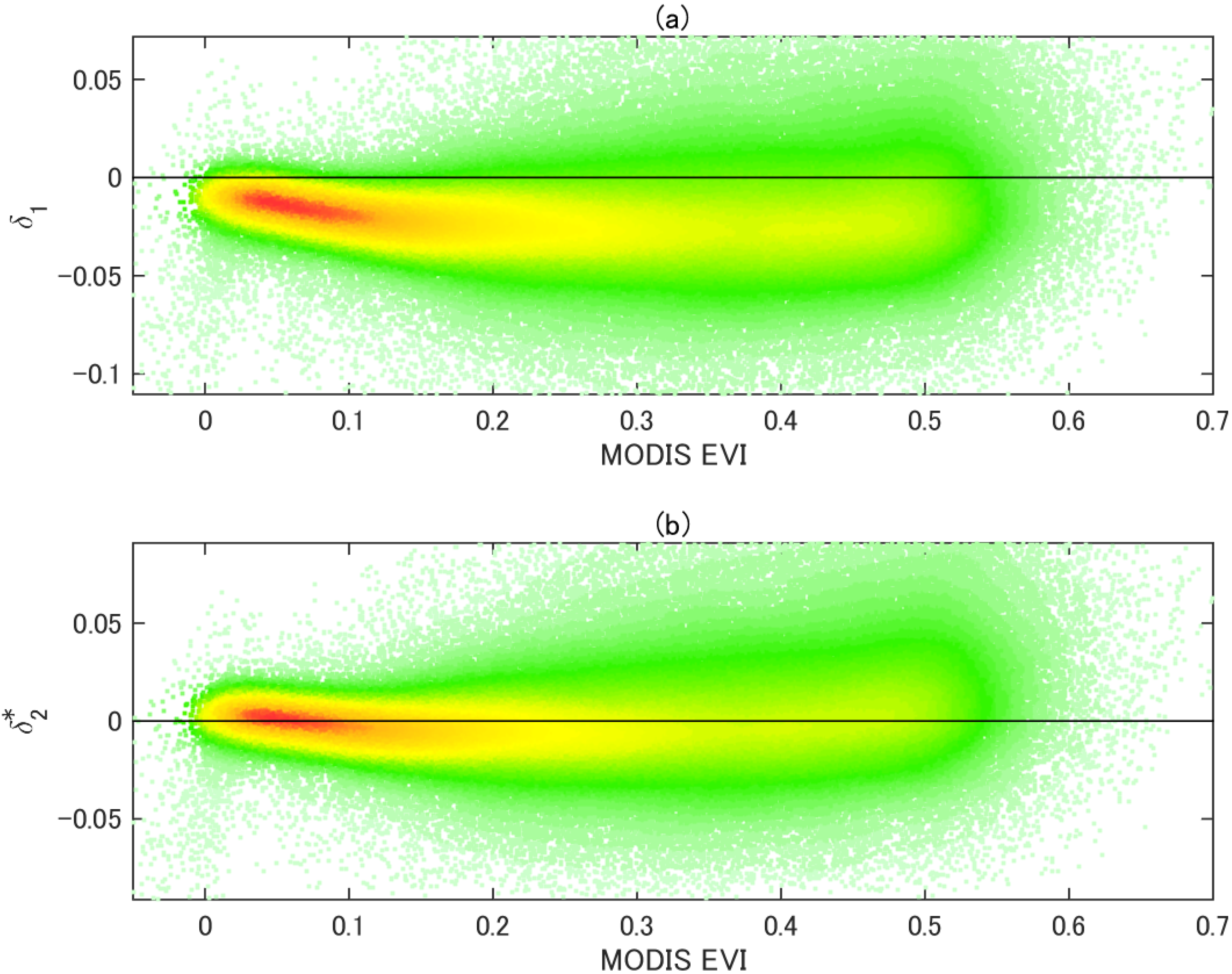
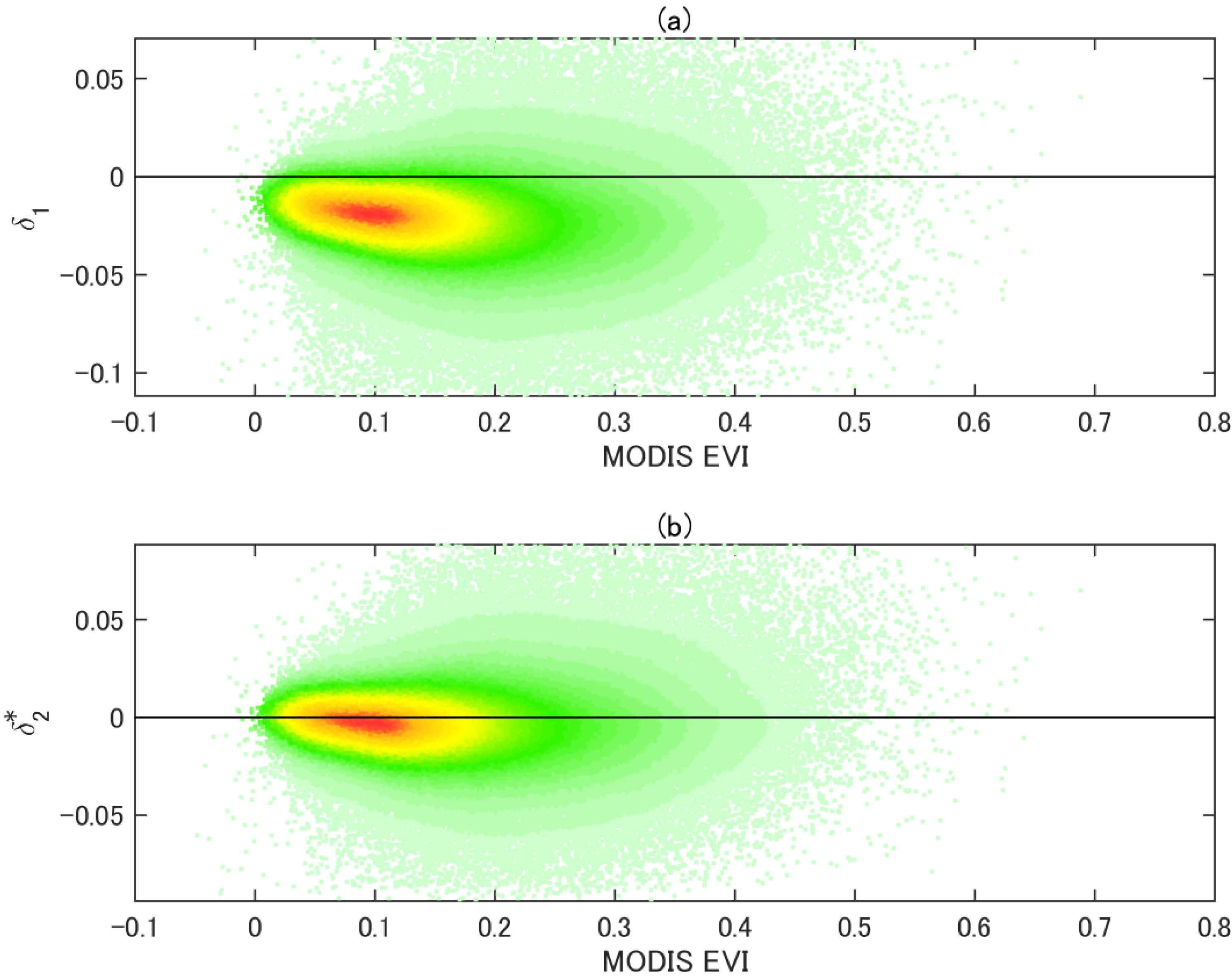
A density plot of MODIS EVI minus VIIRS EVI (
) as a function of MODIS EVI is shown in
Figure 5a. Trends of negative biases and high density in lower EVI values were similar to
Figure 3a but the appearance of the plot (distribution of dots) was different because of different scenarios in extracting sample data. The mean of the error (−0.021) was similar to that obtained from the calibration dataset in
Figure 3a (−0.019), whereas STD and RMSE (0.021 and 0.029) of this evaluation dataset were smaller than those in
Figure 3a (0.028 and 0.034) as summarized in
Table 4.
Figure 5b shows a density plot of MODIS EVI minus MODIS-compatible EVI (
) as a function of MODIS EVI. The absolute average of
(0.003) was reduced from that of
(0.021). STD of
(0.020) was slightly lower than that of
(0.021). RMSE of
(0.020) was reduced from that of
(0.029). These results indicate that the coefficients obtained in the previous section were reasonable.
Figure 5.
Density plots of EVI differences using the data for the evaluation. (a) Density plot of MODIS EVI minus VIIRS EVI () vs. MODIS EVI; (b) Density plot of MODIS EVI minus MODIS-compatible VIIRS EVI () vs. MODIS EVI.
Figure 5.
Density plots of EVI differences using the data for the evaluation. (a) Density plot of MODIS EVI minus VIIRS EVI () vs. MODIS EVI; (b) Density plot of MODIS EVI minus MODIS-compatible VIIRS EVI () vs. MODIS EVI.
Table 4.
Statistics of MODIS EVI minus VIIRS EVI () and MODIS EVI minus MODIS-compatible VIIRS EVI () for the evaluation.
Table 4.
Statistics of MODIS EVI minus VIIRS EVI () and MODIS EVI minus MODIS-compatible VIIRS EVI () for the evaluation.
| | Mean | STD | RMSE |
|---|
| −0.021 | 0.021 | 0.029 |
| −0.003 | 0.020 | 0.020 |
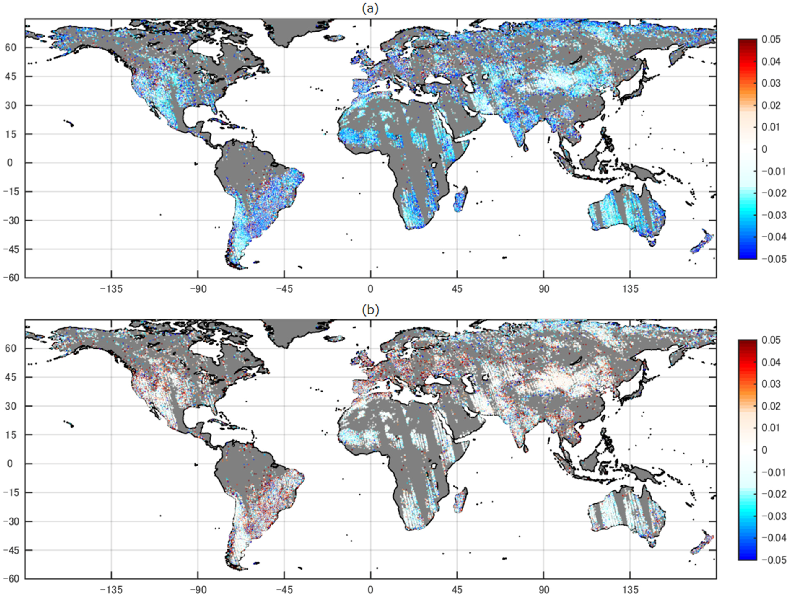
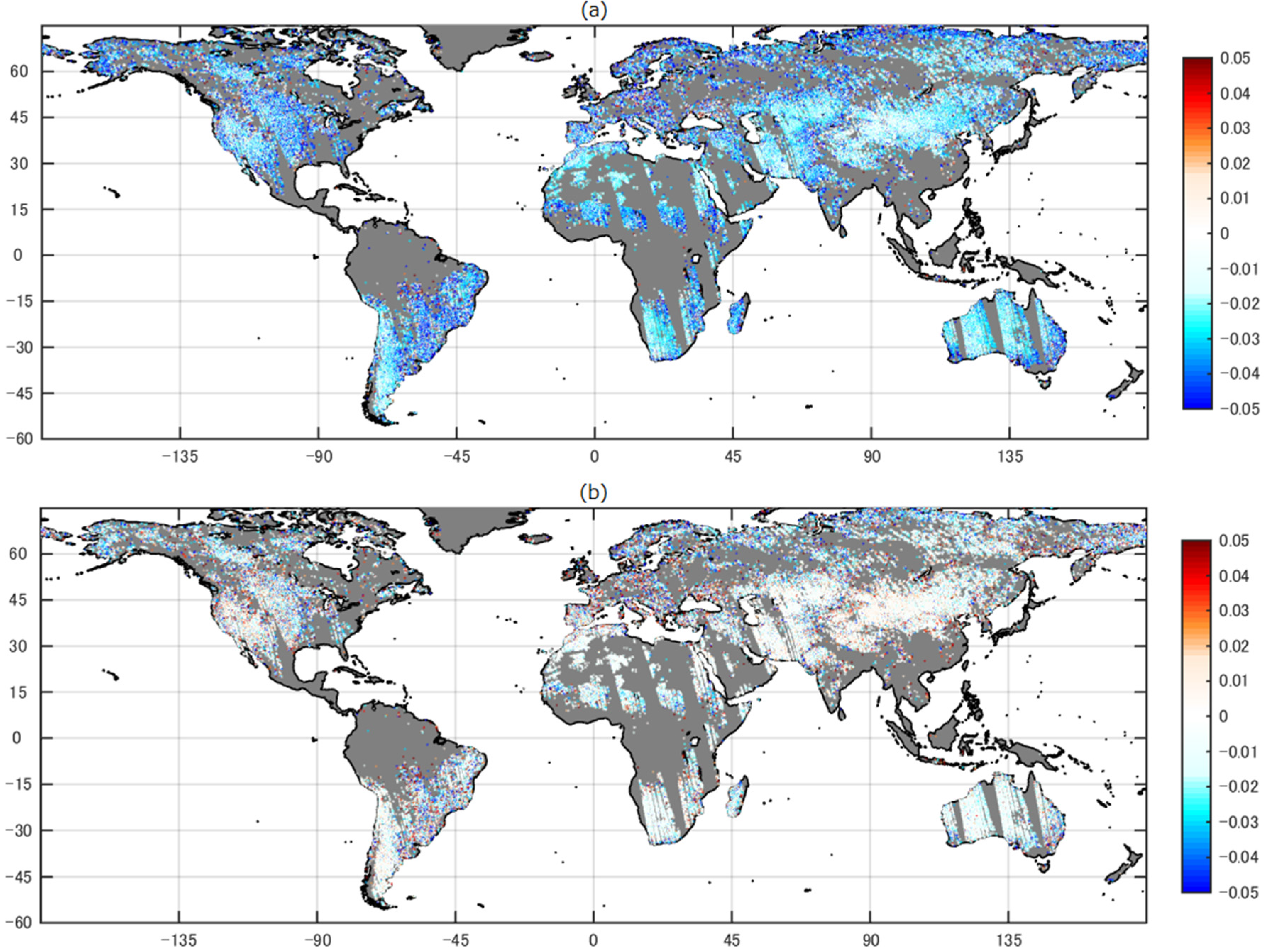
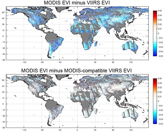
Figure 6a,b show the spatial distribution of MODIS EVI minus VIIRS EVI (
) and MODIS EVI minus MODIS-compatible EVI (
), respectively, for evaluation data. Spatial trends of errors in
Figure 6 are very similar to those in
Figure 4. The spatial coverage of
Figure 6 is slightly wider than
Figure 4 since the sample size of the evaluation dataset (200,000) was larger than that of the calibration/optimization dataset (137,278). The number of positive error occurrences in
Figure 6b appears slightly smaller than that in
Figure 4b because of the two different scenarios used in obtaining the evaluation and calibration datasets. For example, the southern part of the South American continent shows fewer dots of positive errors (red dots) compared to
Figure 4b.
The MODIS-compatible VIIRS EVI was further evaluated by examining its performance with respect to sun-target-sensor viewing angle, EVI dynamic range, and land cover type. Mean, STD, and RMSE of
and
were computed and those of
were divided by the respective counterparts of
, referred to as the ratio of mean (RM), ratio of STD (RS), and ratio of RMSE (RR), for each angle bin, each EVI bin, and each land cover type (
Figure 7,
Figure 8 and
Figure 9, respectively). The MODIS Land Cover Type Yearly CMG (MCD12C1 [
33], resolution of 0.05°-by-0.05°) for 2012 was used to identify the land cover type of each CMG pixel (the 17-class International Geosphere-Biosphere Programme (IGBP) classification) [
34].
Figure 6.
(a) Spatial distribution of MODIS EVI minus VIIRS EVI () over geographic coordinate for the evaluation; (b) Spatial distribution of MODIS EVI minus MODIS-compatible EVI ().
Figure 6.
(a) Spatial distribution of MODIS EVI minus VIIRS EVI () over geographic coordinate for the evaluation; (b) Spatial distribution of MODIS EVI minus MODIS-compatible EVI ().
Figure 7.
(a) Ratio of absolute mean of difference between MODIS EVI minus MODIS-compatible VIIRS EVI () to that between MODIS EVI minus VIIRS EVI () for angular-dependent data (characterized by backward or forward scatterings and view zenith angle); (b) Ratio of STD for to that for ; (c) Ratio of RMSE for to that for ; (d) Frequency of angular distribution in data for evaluation.
Figure 8.
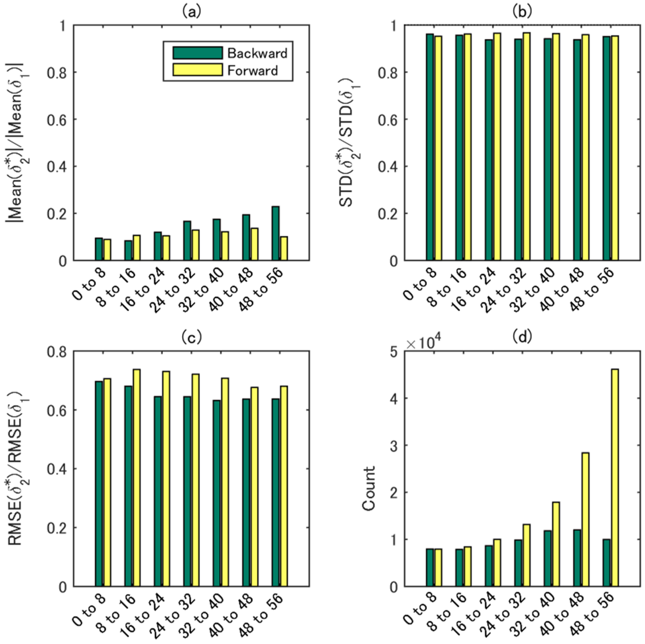
(a) Ratio of absolute mean of difference between MODIS EVI minus MODIS-compatible VIIRS EVI () to that between MODIS EVI minus VIIRS EVI () for EVI-dependent data; (b) Ratio of STD for to that for ; (c) Ratio of RMSE for to that for ; (d) Frequency of EVI distribution in data for evaluation.
Figure 8.
(a) Ratio of absolute mean of difference between MODIS EVI minus MODIS-compatible VIIRS EVI () to that between MODIS EVI minus VIIRS EVI () for EVI-dependent data; (b) Ratio of STD for to that for ; (c) Ratio of RMSE for to that for ; (d) Frequency of EVI distribution in data for evaluation.
Figure 9.
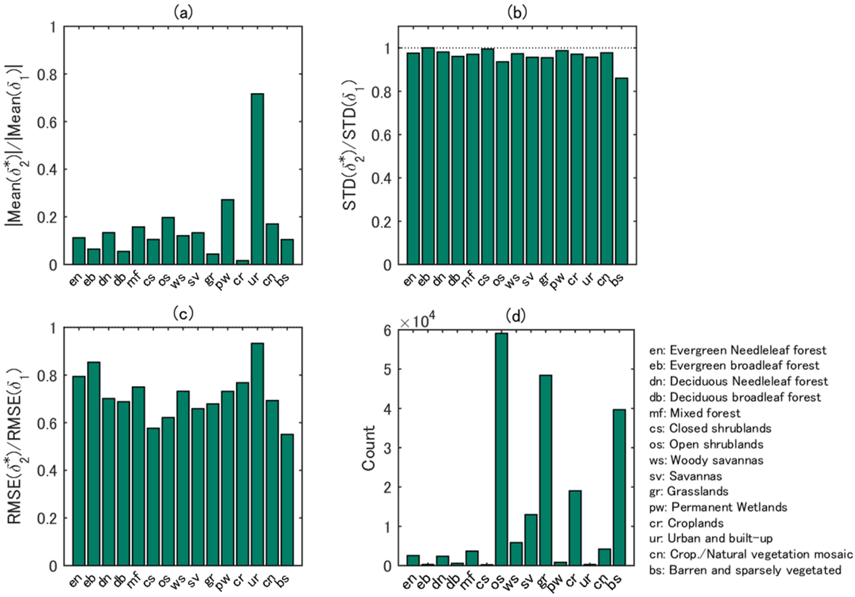
(a) Ratio of absolute mean of difference between MODIS EVI minus MODIS-compatible VIIRS EVI () to that between MODIS EVI minus VIIRS EVI () for land cover-dependent data; (b) Ratio of STD for to that for ; (c) Ratio of RMSE for to that for ; (d) Frequency of land cover type distribution in data for evaluation.
Figure 9.
(a) Ratio of absolute mean of difference between MODIS EVI minus MODIS-compatible VIIRS EVI () to that between MODIS EVI minus VIIRS EVI () for land cover-dependent data; (b) Ratio of STD for to that for ; (c) Ratio of RMSE for to that for ; (d) Frequency of land cover type distribution in data for evaluation.
The RM increased with view zenith angle for the backward scattering geometry, while it remained nearly the same over the view zenith angle range examined here for the forward scattering direction (
Figure 7a). The RS was close to one for both the backward and forward scattering directions, but was slightly smaller for the former than the latter (
Figure 7b). The RR was less than 0.8 and smaller for the backward scattering (
Figure 7c). It tended to decrease with increasing view angles. The MODIS-compatible EVI performed better for the forward scattering direction in terms of bias but better for the backward scattering direction from the perspective of variability.
Figure 7d shows the frequency distribution of each angular condition for this evaluation dataset. The frequency of backward scattering does not show a strong angular dependency, whereas that of forward scattering showed a monotonic increasing trend.
Dependencies of the improvement of RM, RS, and RR on EVI values from MODIS are shown in
Figure 8. Note that the maximum MODIS EVI in our evaluation was 0.688. The RM differed largely across EVI bins (
Figure 8a). The bias was the smallest for the EVI range of 0.3–0.4 and was the largest for higher EVI values (from 0.5 to 0.7). Whereas the RS was less than unity and varied a little across EVI bins (
Figure 8b), the RR varied greatly from 0.5 to 1.25 (
Figure 8c). According to the histogram of this dataset (
Figure 8d), most of samples were in the EVI range between 0 and 0.5. Since the coefficients of the MODIS-compatible VIIRS EVI are sensitive to canopy greenness [
17], a smaller number of samples in higher EVI values would have been a source of the large RM and RR for that EVI value range. It should be noted that cloud leakage in VCM could degrade the performance of the atmospheric correction algorithm, which may likely be associated with densely vegetated areas due to persistent cloud coverage.
Land cover dependencies of RM, RS, and RR are shown in
Figures 9a–c, respectively. Note that data corresponding to “Water” and “Permanent snow and ice” were excluded from this evaluation. The RM was less than 0.4 except for the urban and built-up (ur) cover type (
Figure 9a). The RS was close to unity (
Figure 9b). The RR was smaller than unity, and showed large improvements for barren and sparsely vegetated area (bs), closed shrublands (cs), and open shrublands (os) followed by savanna (sv) and grass land (gr) (
Figure 9c). The urban and built-up area, in general, shows totally different spectral characteristics from vegetated areas, which might have caused the largest RM and RR.
Figure 9d shows the land cover frequency of this evaluation dataset. The sample sizes of os, gr, and bs were large, and a general negative correlation between the sample size and the improvements in statistics was observed. The forest cover types where high EVI values are expected (first five cover types in
Figure 9a–d) showed some improvements in the statistics, although samples with large EVI values resulted in larger errors. The MODIS/VIIRS EVI tended to fall approximately between 0.1 and 0.5 (0.25 in average) for forest types, in which the MODIS-compatible VIIRS EVI showed higher performance than in the higher EVI value range.
5. Discussions
The coefficients obtained through the calibration/optimization using the one-year global dataset were (
,
,
,
) = (1.026, −0.001, 0.874, 1.022). The optimum coefficients obtained for North America in August 2013 in our previous study [
17], represented here by
(
= 1, 2, 3, 4), were (
,
,
,
) = (0.947, 0.010, 0.265, 0.995). These differences in the optimum coefficient values resulted from the spatiotemporal coverages of the calibration datasets used in the present and previous studies. It should be noted that
obtained in this study fell in or approached the range of coefficients simulated by radiative transfer models (PROSAIL and 6S code) [
17]. The maximum and minimum of
(
= 1, 2, 3, 4) obtained in the model simulation were (0.980, 1.024), (−0.002, 0.004), (0.695, 0.935), (0.879, 1.020), respectively.
(−0.001) and
(0.874) fell within their corresponding ranges, and
(1.026) and
(1.022) slightly greater than the ranges. Since the simulation of coefficients was performed by varying optical thickness of vegetation canopy and aerosol layer but by fixing angular condition, considerations of angular variations in the present study could widen the ranges of coefficients characterized by the maximum and minimum to include
obtained in this study. Further investigation is required to fully understand the relationship between the optimum
values from actual sensor data and ranges of coefficients simulated using radiative transfer models.
The derived equation of MODIS-compatible VIIRS EVI was a non-linear function of
, and therefore the optimization of
corresponds to the non-linear regression. The small non-linear biases, however, still remained in the
(MODIS EVI minus MODIS-compatible VIIRS EVI) in
Figure 3b. The comparison of our algorithm with alternative models such as polynomials is certainly important and worthy to evaluate, which is a focus of future work.
The calibrated MODIS-compatible VIIRS EVI showed less compatibility with MODIS EVI over higher EVI values (
0.5). MODIS-VIIRS reflectance pairs that had large positive values in
(MODIS EVI minus MODIS-compatible EVI) also had positive values in
(MODIS EVI minus VIIRSE EVI). However, a Hyperion-based bandpass simulation analysis conducted over AERONET sites only found negative values in MODIS EVI minus VIIRS EVI [
15]. This discrepancy implies that these large positive
values were likely caused by other potential factors than the bandpass differences, such as cloud leakage in VCM which decreases VIIRS EVI and increases
and
, and the maturity status (quality level) of the input surface reflectance data.
The VIIRS surface reflectance product was on a “beta” maturity status for the data period used in this study. Likewise, the VIIRS sensor data record (SDR), the input to the VIIRS surface reflectance product, reached a provisional status in March 2013 [
31]. Quality issues associated with the VIIRS surface reflectance data that we noticed included cloud leakage [
17,
35], aerosol optical thickness [
36,
37], and VIIRS algorithmic differences from MODIS. The leakage of small clouds resulted in large biases in the surface reflectance intermediate product (IP) which were not documented in QFs [
16]. Therefore, spatial averaging for generating CMG pixels could have operated differently between MODIS and VIIRS due primarily to the cloud leakage in VCM. The MODIS/VIIRS pixels involved in area-averaging for generating CMG pixels heavily depend on algorithmic accuracy for cloud detection over the cloudy area. Such dependency caused the situation that the number of pixels,
i.e., the areas used to compute CMG reflectances, was not identical between sensors even if the area for the averaging (0.05°-by-0.05°) was the same location. This could subsequently impose substantial differences between CMG reflectances of sensors, in addition to cloud contamination. Significant improvements have, however, been made to these input products since the commencement of this study and additional improvements are planned (e.g., [
38,
39]). The same and additional analyses using the VIIRS surface reflectance product with a higher maturity status (e.g., provisional or validated stage-1) should allow to examine and identify the factor(s) that caused this apparent poor calibration results for high EVI values and to obtain more refined calibration results of the equation/coefficients.
Coefficients in the MODIS-compatible EVI to be optimized are also influenced by characteristics in sample data and an optimization algorithm. The sample data are characterized by several factors including maturity (accuracy) of the product, the number of samples, frequencies in sun-target-viewing geometry, observation time period, and land cover types. The optimization of coefficients depends on the merit function and the algorithm to search for the optimum solution. The algorithm comprised by the merit function of MAD and the search algorithm of the Nelder-Mead simplex method starting from multiple initial guesses performed properly for the problem of the EVI optimization, which involves multiple local minima.


