Evolutionary View Planning for Optimized UAV Terrain Modeling in a Simulated Environment

Abstract

This work demonstrates the use of genetic algorithms in optimized view planning for 3D reconstruction applications using small unmanned aerial vehicles (UAVs). The quality of UAV site models is currently highly dependent on manual pilot operations or grid-based automation solutions. When applied to 3D structures, these approaches can result in gaps in the total coverage or inconsistency in final model resolution. Genetic algorithms can effectively explore the search space to locate image positions that produce high quality models in terms of coverage and accuracy. A fitness function is defined, and optimization parameters are selected through semi-exhaustive search. A novel simulation environment for evaluating view plans is demonstrated using terrain generation software. The view planning algorithm is tested in two separate simulation cases: a water drainage structure and a reservoir levee, as representative samples of infrastructure monitoring. The optimized flight plan is compared against three alternate flight plans in each case. The optimized view plan is found to yield terrain models with up to 43% greater accuracy than a standard grid flight pattern, while maintaining comparable coverage and completeness.

1. Introduction

Unmanned aerial vehicles, or UAVs, are useful remote-sensing platforms for infrastructure monitoring and inspection. The small size and maneuverability of UAVs make them highly mobile sensor platforms that can quickly and easily gather information about an environment that would otherwise be difficult to obtain. UAVs provide promising applications in many fields and are providing increasingly valuable services to industry. Although historically, UAVs have been used largely in military applications, new industrial opportunities may utilize UAVs as remote-sensing tools in areas as diverse as precision agriculture, landslide observation, pipeline surveillance, photogrammetric modeling and infrastructure monitoring [1,2,3,4,5,6,7]. UAVs have an advantage over manned aircraft in these applications due to autonomy, the ability to capture data at close range and high resolution and reduced cost [8].

One particularly attractive use of UAVs for many industries is as a highly mobile sensor platform for 3D reconstruction [9]. Images collected during UAV missions can be processed to create 3D models of a scene using techniques, such as structure from motion (SfM) [10]. The resulting models are useful for observation of terrain changes [11], inspection of existing infrastructure [12] and environmental monitoring [13].

Currently, many civilian UAV missions are flown using manual pilot control, making the quality of the collected data heavily dependent on the skill and judgment of the operator or the weather conditions that make precision flying more difficult. This can often lead to gaps between the collected images or areas where insufficient images are captured for 3D reconstruction. 3D reconstruction using SfM, for example, is particularly sensitive to the overlap and angles of the provided images [14]. Although automated flights are becoming increasingly more common, most widely-available flight planners use a simple grid or “lawnmower” flight pattern. While easily adjustable, these patterns often take little account of the 3D geometry of a scene, leading to potential gaps and areas of reduced accuracy. These problems are alleviated through a new view planning optimization algorithm described in this paper.

View planning refers to identifying the best sensor locations for observing an object or site and is also known as active vision, active sensing, active perception or a photogrammetric network design [15]. Early approaches have roots in the “art gallery” problem, which deals with optimally placing museum guards to protect an exhibit [16]. Other early motivations included industrial inspection and quality control for parts manufacturing [17].

View planning is divided into two general categories: model-based and exploratory. Exploratory view planning, also known as next-best view planning, does not rely on any prior knowledge about the scene. Early works on the subject include that of Remagnino et al. on active camera control [18] and Kristensen on sensor planning in partially-known environments [19]. Dunn and Frahm develop an algorithm for next-best view planning in generic scenes [20]. Krainin et al. present an active vision planner in which a robot manipulates an object in front of the camera to achieve a complete inspection [21]. Some work, such as that by Trummer et al. and Wenhardt et al., has also been performed using various uncertainty criteria to plan the next viewing position for the sensor [22,23].

This research deals primarily with model-based view planning, which presumes some prior knowledge about the scene. For UAV applications, this is a good assumption, as rough elevation data are generally available for most areas of interest to Earth science and infrastructure monitoring. Furthermore, view planning is effective even with only a simplified version of the model geometry [24]. In UAV applications, a rough model may also be created quickly using a pre-programmed flyover of the area [14].

Early works in model-based view planning include those by Cowan and Koveski [25], Tarbox and Gottschlich [26] and Tarabanis et al. [27]. Model-based view planning consists of two parts [28]. The first is the generation and selection of an acceptable set of viewpoints to cover the scene. The second is the calculation of a path to reach the desired viewpoints efficiently. The second step is also known as the traveling salesman problem (TSP). These steps can occur separately or simultaneously in a global optimization. A global solution is desirable, but often impractical to compute [29]. The current work follows the common approach of decoupling the two steps into separate optimization problems. Scott showed that model-based view planning is analogous to the set covering problem, which is NP-complete [30]. NP refers to nondeterministic polynomial time. NP-complete is a class containing the hardest problems in NP. This classification means while any given solution can be quickly checked, no known, efficient method for finding a solution exists. For more information, see [31]. Although the view planning problem is complex, a number of researchers have proposed potential solutions that approach optimality.

Scott (2007) presents a theoretical framework for model-based view planning for range cameras. He poses the problem as a set covering problem and develops a four-part “modified measurability matrix” algorithm for its solution. He separates viewpoint selection and path planning, using a greedy algorithm to solve the first and a heuristic approximation algorithm to solve the second. Greedy algorithms work by choosing a locally-optimal option at each decision stage. Heuristic algorithms utilize “rules of thumb” that can produce good results, but have no guarantees of optimality. Neither algorithm guarantees a global optimum, but are instead chosen by Scott as a balance between solution quality and efficiency [32]. Due to the general nature of this work, these results can be extended to other sensor types in addition to range scanners. The components of the fitness function described in Section 2.1.4 of the current work are derived in part from Scott’s measurability criteria.

Blaer and Allen (2007) perform view planning for ground robot site inspections using a unique voxel space and ray tracing approach to represent the solution space. The robot first uses a 2D site map to plan an initial inspection path and generate a rough 3D map. Viewpoints are then selected sequentially using a greedy algorithm, and the robot path is generated using a Voronoi diagram-based method. The authors test their algorithm on a large historic structure. Their tests show the algorithm to be effective, but quite slow, requiring 15–20 min to compute the next viewpoint [33].

The field of photogrammetric network design closely overlaps the field of view planning, but focuses more closely on the requirements taken from photogrammetry for accurate reconstruction. This type of design aims for well-distributed imaging network geometry and often employs carefully-designed targets and scale bars. This approach has been shown to produce very good results in small scenes, with Alsadik et al. demonstrating accuracies of up to 1 mm in cultural heritage preservation projects [34,35]. The current work does not attempt to produce a rigorous network design, focusing instead on providing sufficient coverage of large scenes for 3D reconstruction to take place.

Scott et al. identify highly mobile, six degree of freedom positioning systems as an open problem in view planning research [30]. UAVs fill that need, but introduce additional challenges. Past work in view planning often focuses on small-scale industrial inspections, where a fixed robotic positioning system manipulates the sensor. The size of the inspected object in such systems rarely exceeds the sensor viewing area [24]. However, in UAV applications, the observed surface is often much larger than the sensor viewing area. Work done on view planning for site inspection commonly uses ground robots, with viewpoints in a 2D plane [36,37]. In contrast, UAVs move in three dimensions, allowing viewpoints in an additional dimension. As a result, UAV view plans require more viewpoints to cover a 3D surface. This increases the computational complexity compared to that for the manufacturing inspection case for some portions of the view planning process, including visibility analysis, view point selection and the traveling salesman problem [15].

Some work addresses these challenges. Schmid et al. present a multicopter view planning algorithm that uses a heuristic view selection approach to create a set of viewpoints [14]. The viewpoints cover a desired area while meeting the constraints for multi-view stereo reconstruction. The algorithm approximates the shortest path to the chosen viewpoints using a farthest-insertion-heuristic. The authors test the algorithm on a medium- and a large-scale scene with acceptable results for 2.5D reconstructions. However, while model resolution is reported, no qualitative analysis is performed to establish the accuracy of the models. Hoppe et al. develop a similar algorithm that differs by including an analysis of anticipated reconstruction error using the E -optimality criterion, which maximizes the minimum eigenvalue of the information matrix. They plan the path using a greedy algorithm with angle constraints and test their algorithm on a house under construction. The authors obtain errors of less than 5 cm across 92% of the reconstructed points [38]. Both of these projects are closely related to the current work and provide alternate methods for achieving similar goals. The lack of numerical analysis by Schmid et al. makes direct comparison difficult, but the results of the current paper are compared to those obtained by Hoppe et al. in Section 4.

In a more theoretically-based approach, Englot and Hover present a view planning algorithm for underwater robot inspections, which share a common scale and dimensionality with many UAV planning problems. The solution to the set cover problem is found using both a greedy algorithm and linear programming relaxation with rounding. The algorithm efficiently computes a sensor plan that gives 100% coverage of complex structures [39]. In a subsequent paper, the authors revisit the same problem, this time fitting the input model with a Gaussian surface, modeling uncertainty in the surface using Bayesian regression and planning views that minimize uncertainty in the surface [40]. This is related to the objective of the fitness function in the current work, which seeks to maximize the number of terrain point locations that can successfully be estimated using SfM.

A promising approach for large-scale view planning is evolutionary or genetic algorithms, which use stochastic processes to iteratively progress toward an optimum. Genetic algorithms are especially useful in this application because of the nonlinear and non-convex nature of the problem, which can cause difficulties for traditional gradient-based optimization techniques [17]. Olague uses this approach to develop a camera network design for a robotic camera positioning system [41]. Chen and Li (2004) also apply this approach, using a genetic algorithm to choose viewpoint sets with a min-max objective. The viewpoint sets are evaluated based on the number of viewpoints, the visibility of model features and sensor constraints [17]. Once a set of viewpoints is selected, the shortest path is estimated using the Christofides algorithm, which provides a solution no greater than three halves of the optimum [42].

In a study closely related to the subject of this paper, Yang et al. develop a genetic optimization algorithm that selects camera positions for UAV inspection of transmission tower equipment [43]. The algorithm discretizes both the tower and a cylindrical surface around the tower. Each point on the cylindrical surface becomes a potential viewpoint. The genetic algorithm then searches for the optimal viewpoint for each portion of the tower surface, evaluating viewpoints based on visibility, viewing quality and distance. The optimized viewpoints are then compared to an evenly-distributed set of viewpoints. The authors found that the optimized viewpoints performed better than the evenly-distributed set in all three evaluation metrics. The current project performs similar tests for terrain features and structures and additionally adds image orientation to the list of optimized variables.

The current study extends and improves upon previous work by using a genetic algorithm for view planning in a large and unstructured environments common in UAV terrain modeling [44]. Contrasting with previous evolutionary-based work, the view space is formulated as continuous rather than discretized, allowing more flexibility in the solution and the possibility of a more optimal result [45]. A novel simulation environment using terrain-generation software is also developed for UAV view plan testing. In addition, a quantitative analysis is performed to compare the models created using an optimal view set to those created using three alternative flight patterns in terms of both accuracy, coverage and model completeness.

2. Materials and Methods

2.1. Genetic Algorithm

Genetic algorithms are a type of evolutionary computation distinguished by an initial population of solutions which is manipulated by several operators to progress toward an optimal solution over a series of generations. These operators include selection according to a fitness function, crossover to create new solutions and random mutation of new solutions [46]. The objective of the algorithm is to explore the search space of the problem, combining the best aspects of each solution found. This section describes the details of the genetic algorithm used in this project.

2.1.1. Terrain Data Acquisition

The presented algorithm is a model-based view planner, meaning that it acts on the assumption that some initial information is known about the site before planning begins. In this case, elevation data at 10-m resolution from the U.S. Geological Survey (USGS) National Elevation Dataset are used to provide the general shape of the terrain being reconstructed [47]. First, the region of interest (ROI) is selected in Google Earth and saved as a Keyhole Markup Language (KML) file. The KML file is loaded in MATLAB, and elevation data in an area surrounding the ROI are downloaded from the appropriate Web Map Service (WMS) server.

2.1.2. Initialization

The initial population of solutions for the genetic algorithm is initialized through a seeded approach. For the purposes of this project, a solution is defined as a set of image positions and orientations representing a UAV flight. Position here is defined in terms of northing, easting and altitude, while orientation is defined by the azimuth and elevation angles of the image. Roll is neglected for simplicity and easy application of the results to planned future flight tests using a single axis camera gimbal. Each solution thus has 5n decision variables, where n is the number of images in the flight. The population then consists of N solutions, where N is the population size. Figure 1 shows an example of a single solution for a terrain area. The solution is composed of 48 image locations and their corresponding orientations.

Figure 1. Illustration of a sample solution, comprising 48 image positions denoted as black triangles and their orientations shown as red dashed lines.

Figure 1. Illustration of a sample solution, comprising 48 image positions denoted as black triangles and their orientations shown as red dashed lines.

The population is first initialized by randomly generating a set of solutions. Each image position is then automatically evaluated to determine if it contains any points in the ROI. If it does not, it is discarded, and another image is generated. This brute force initialization is not very efficient. However, the initialization step takes only a small fraction of the total run time, so this method is acceptable from a computational standpoint.

In addition to random generation, the initial population is also seeded using a noisy grid pattern. The image grid is generated with commonly-used values of 75% frontal overlap and 60% side overlap. Recommendations on image overlap vary, but these settings are in line with most current standards of best practice [48,49,50,51,52]. Random noise of ±5 m and ±5 degrees is then added to the position and orientation of each image in the grid to produce a perturbed grid pattern. This is repeated to produce a large number of different perturbed grid patterns. Half of the initial population is then replaced with these perturbed grids. The authors have found that this seeding helps to introduce some structure into the evolving solution, as well as image network geometry and leads to a more optimal result. The initial grid pattern, as well as the first perturbed grid solution are set aside for later comparison with the final solution.

2.1.3. Parameter Tuning

The operation of a genetic algorithm is influenced by a number of parameters that can be tuned to the specific problem to be solved. The population size controls the number of solutions calculated in each iteration of the algorithm. The crossover probability controls the probability that variables from a set of two solutions will be combined in the next iteration to promote good solutions. The mutation probability describes the probability that some solution variables will be changed semi-randomly to maintain a diverse set of solutions. The dynamic mutation parameter causes mutation to occur less frequently the longer the algorithm runs, to promote convergence. Another important parameter to consider is the total number of generations or iterations that the algorithm runs. This is determined while the algorithm is running by the convergence criteria described in Section 2.1.4.

Tuning parameters for the genetic algorithm were selected through semi-exhaustive search of the parameter space. Multiple optimizations were performed on a small set of test data, stopping the algorithm after a fixed number of generations. The results of the tests were tabulated, and Table 1 contains the parameters that produced the best and most consistent results over the small set of test data. These parameters were used throughout the remainder of the study and are described in greater detail in the subsequent section.

Table 1. Algorithm tuning parameters.

Parameter	Value
Population Size	30
Crossover Probability	0.70
Mutation Probability	0.05
Dynamic Mutation Parameter	1

Table 1. Algorithm tuning parameters.

Parameter	Value
Population Size	30
Crossover Probability	0.70
Mutation Probability	0.05
Dynamic Mutation Parameter	1

2.1.4. Genetic Algorithm Implementation

The genetic algorithm used for the view plan optimization is detailed in the following sections that describe the fitness (objective) function, how inheritance is transferred from one generation (iteration) to another, diversity in the initial guess and the introduction of diversity throughout the generations, preservation of best solutions through elitism and details on the qualifications for convergence.

Fitness Function

The progress of a genetic algorithm towards a more optimal solution is driven by a fitness function that assigns a score to each candidate solution. This fitness score represents the relative merit of each solution in meeting the problem objectives. The fitness function for this system is based on the requirements for the 3D reconstruction of a scene using structure from motion algorithms. The fitness scoring function f is given in Equation (1), where C represents coverage and F_c represents the functional coverage. These two quantities are described in the following paragraphs.

$$f=C+F_c$$

(1)

Coverage, in this sense, is defined as the number of visible terrain points v in the images of a solution set divided by the total number of terrain points T, as in Equation (2). Coverage can also be described as percent viewable.

$$C=\frac{v}{T}$$

(2)

Visible terrain points are those within the field of view of at least one image in the set. A maximum camera range is also defined for visibility purposes as the distance from the camera at which the ground sampling distance (GSD), or distance between pixels, is equal to the desired GSD of the flight. Terrain points beyond this range are considered invisible. Functional coverage is a subset of coverage and accounts for the need to capture terrain points from multiple angles to achieve an accurate 3D reconstruction. First, the normal of each point on the terrain is calculated. Then, for each point, the images that contain the point are sorted according to their angle away from the point normal using a histogram function with edges at (0°, 10°, 20°, 30°, 40°). The concept is illustrated in Figure 2.

Figure 2. Illustration of the image angle histogram used in the functional coverage metric.

Figure 2. Illustration of the image angle histogram used in the functional coverage metric.

Points with images in at least three of the histogram bins are visible from at least three angles near the surface normal and are considered functionally covered for the purposes of 3D reconstruction. The variable P is defined as the number of points in the terrain meeting these criteria. The total functional coverage is then computed by normalizing P by dividing by the total number of terrain points T, as shown in Equation (3). Functional coverage can also be described as percent reconstructable.

$$F_c=\frac{P}{T}$$

(3)

The combination of coverage and functional coverage in the fitness function was chosen due to the use of both SfM feature matching and multi-view stereo (MVS) in the reconstruction pipeline. The first relies heavily on multiple imaging angles to locate points in space, while the second requires only stereo pairs for dense reconstruction.

Inheritance

Two solutions are randomly selected as a mother and father. Once a pair of parent solutions is selected, blend crossover is performed with a crossover probability of 0.7. For each image in the pair of solutions, a new image is created by computing a weighted average of the image position, defined by northing, easting and elevation, as well as the image azimuth and elevation, which define the orientation. To avoid large perturbations in the population, when an image pair is selected for crossover, each of the five image variables has a 50% chance of participating in the crossover process. The crossover process is demonstrated in Equations (4) and (5) for the elevation crossover, where r is a random number between zero and one. The two new images thus form a convex combination of the two original images. This is repeated for each image until two new sets of solutions are created from the parents.

new image A elevation = r(mother image elevation) + (1 − r)( father image elevation)

(4)

new image B elevation = (1 − r)(mother image elevation) + r(father image elevation)

(5)

Diversity

A tournament selection was initially used to choose parent solutions; however, it was found that seeding the population with the grid solution caused a premature loss of diversity in the population in combination with the tournament. Because of this, a simple random selection is implemented to maintain diversity. As an additional measure to ensure diversity in the population of solutions, crossover is followed by mutation with an initial mutation probability of 5%. Mutation is applied to all solution variables, including image northing, easting and elevation, as well as azimuth and elevation. Dynamic mutation is implemented with a dynamic parameter α of one, meaning that solution variables are initially perturbed to random values anywhere within the variable bounds, but that the magnitude of perturbation decreases throughout the duration of the optimization. Equations (6) and (7) describe an example of the mutation process for the image easting. Here, α is the dynamic mutation parameter, a is an intermediate variable related to the dynamic mutation, g is the current generation number, G is the total number of generations, E is the current image easting, E_new is the new image easting, E_max is the maximum allowable northing, E_min is the minimum allowable northing and r_e is a random number between E_min and E_max.

$$a={\left(1-\frac{g-1}{G}\right)}^{\alpha }$$

(6)

$$E_{new}=\left\{\begin{array}{ll}{E}_{new}=E_{min}+{(r_e-E_{min})}^a{(E-E_{min})}^{1-a}& \text{if}{r}_e\le E\\ E_{new}=E_{max}-{(E_{max}-r_e)}^a{(E_{max}-E)}^{1-a}& \text{otherwise}\end{array}\right.$$

(7)

Elitism

To drive the solution population more quickly towards an optimum, elitism is implemented, meaning that good parent solutions are propagated to the child. In this implementation, the parent and child populations were sorted individually according to score. The lowest ranking 25% of solutions in the child population are then replaced with the highest ranking 25% of solutions in the parent population. This requirement helps ensure that good potential solutions are preserved.

Convergence

At each generation, the algorithm is tested for convergence according to the condition given in Equation (8), where a_c is the average score of the current generation and m is the mean of the average scores of the last ten generations.

$$\frac{\left|a_c-m\right|}{a_c}<0.00005$$

(8)

Once the algorithm has converged, the final solution is improved by removing any images that cannot see any terrain points, as well as any image locations under the terrain.

2.1.5. Path Planning

Once the optimal set of viewpoints has been planned, the shortest path to visit all of the waypoints may be computed by solving a three-dimensional traveling salesman problem (TSP). There are variety of solution approaches and approximations to the TSP, and they are not treated in this study [53,54,55,56]. Because of the relatively small number of waypoints involved in the studied cases, the TSP is formulated as a binary integer linear program and is solved through branch and bound using the mixed integer linear programming solver available in the MATLAB software package. This approach, while computationally prohibitive for a large TSP, provides an exact solution and is considered sufficient for the current study.

2.2. Simulation Environment and Model Analysis

In the course of developing the presented UAV view planning algorithm, the authors found it essential to provide an environment capable of evaluating the strengths and weaknesses of proposed view plans without the expense, risk and time required by physical flight tests. To this end, a terrain generation software is used to create simulated versions of sites of future interest. For the purposes of this study, Terragen 3 was chosen as the terrain generation software, due to its capacity for fine control of camera properties and positioning. Additional capabilities, such as detailed control of environmental lighting and atmospheric effects, were not used in this study, but provide interesting possibilities for future work.

First, elevation data are acquired at the highest resolution available for the desired site and draped with high resolution orthoimagery. Even so, the resulting terrain is often very smooth, which, combined with limited detail in the draped imagery, can lead to images with very few distinct features and little texture. This makes it difficult for SfM algorithms to extract the keypoints required for 3D reconstruction. To remedy this, fine fractal deformation is applied to the surface, adding geometric noise to approximate the level of detail available to an SfM algorithm in the real world. An example of this is shown in Figure 3.

Figure 3. Addition of random fractal noise to artificially increase simulated terrain detail. Without (a) and with (b) added fractal noise.

Figure 3. Addition of random fractal noise to artificially increase simulated terrain detail. Without (a) and with (b) added fractal noise.

Once the simulated terrain has been created, images are rendered from the desired viewpoints using a virtual camera. The specifications of the camera can be adjusted to match any physical camera chosen. The images are then processed using Agisoft Photoscan, a commonly-used software package in the field. The program settings used to create the models are detailed in Table 2. The models were processed without ground control points and using self-calibrating bundle adjustment. This means that the software was allowed to estimate all camera parameters during the reconstruction process. The end result of the process is a dense 3D point cloud model of the simulated terrain.

One of the main advantages of the simulated environment is that the original geometry of the simulated terrain is known exactly and can be exported as a point cloud. This allows for a very accurate comparison between models produced using different view plans. Figure 4 illustrates the way in which the simulated testing process parallels the way in which physical tests would be performed.

Table 2. Program settings for model reconstruction.

Photo alignment	High
Pair preselection	Disabled
Key point limit	100,000,000
Tie point limit	10,000
Dense cloud quality	High
Depth filtering	Mild
Mesh surface type	Arbitrary
Source data	Dense cloud
Face count	High

Table 2. Program settings for model reconstruction.

Photo alignment	High
Pair preselection	Disabled
Key point limit	100,000,000
Tie point limit	10,000
Dense cloud quality	High
Depth filtering	Mild
Mesh surface type	Arbitrary
Source data	Dense cloud
Face count	High

Figure 4. Relationship between simulated and physical view plan testing.

Figure 4. Relationship between simulated and physical view plan testing.

To measure the performance of the algorithm, the point cloud models created in Agisoft are compared against the original terrain exported from the terrain generator, referred to here as the ground truth model. The comparison is performed in the open source software Cloud Compare [57]. Two metrics are computed and compared for each model: accuracy and model completeness.

The first metric, accuracy, reflects the error between the model geometry and reality. This is determined by comparison with the ground truth model. The scale of the ground truth model is identical to the scale of the original elevation data and is assumed to be correct. The Agisoft point cloud model is first roughly aligned to the ground truth by manually picking four pairs of corresponding points on each model. The points chosen are distinctive features, such as corners of sidewalks or roads that are easy to identify in each model. The compared model is then automatically rotated and scaled to align the chosen points with the corresponding set on the ground truth. Once the two models are roughly aligned, fine alignment is performed using the iterative closest point (ICP) algorithm [58]. The ICP algorithm minimizes the distance between two point clouds by using a mean squared error cost function to estimate the rotation, translation and scaling that most closely aligns the two clouds. Once the two clouds are aligned, the distance between each point in the model and the surface of the ground truth model is computed using a local quadratic fitting technique. This technique finds the distance between a point in the compared cloud and the surface interpolated from its nearest neighbors in the reference cloud. The technique is illustrated in Figure 5. The fitting technique is used due to the increased accuracy it provides over a simple nearest neighbor approach.

Following the distance computations, the cloud to cloud distances are fit with a Gaussian distribution, and the mean error is determined for each view set.

The second metric computed is the model completeness. This metric quantifies the gaps or holes in a model, as well as areas of low model density. These reconstruction failures can occur for a number of reasons, including insufficient source photos of an area, blurry photos, poor lighting or homogeneous textures, such as smooth metal or cement surfaces. As fewer holes and greater point density generally lead to a more useful model, it is desirable to maximize the model completeness.

Figure 5. Illustration of the quadratic fitting technique used to find the distance between the reference cloud (black) and the compared cloud (blue).

Figure 5. Illustration of the quadratic fitting technique used to find the distance between the reference cloud (black) and the compared cloud (blue).

The model completeness is computed for each model through the following process. First, the completed point cloud model is filtered to remove outliers, and the average point spacing is determined. The point cloud is then meshed using Poisson surface reconstruction, filling any holes through interpolation [59]. A new point cloud is then sampled uniformly from the mesh. This produces a point cloud without any holes or gaps. The mesh point cloud is aligned precisely with the original, and a nearest neighbor distance computation is performed between each point in the mesh point cloud and the original cloud. The resulting distances are then filtered to include only those points with distances greater than the average point spacing of the original cloud. This results in a subset group of points from the mesh cloud corresponding to the holes in the original model and areas of low point density. This concept is shown in Figure 6.

Figure 6. Illustration of the model completeness metric showing the model with terrain points shown in blue and hole points highlighted in red (a); and terrain points without highlighted holes (b).

Figure 6. Illustration of the model completeness metric showing the model with terrain points shown in blue and hole points highlighted in red (a); and terrain points without highlighted holes (b).

Because the mesh cloud is evenly sampled, the ratio between the number of points in the filtered subset and the total points is equal to the percentage of the original model consisting of holes. From this information, the percentage of the original model not consisting of holes or low density sections is found.

3. Results

The genetic view planning algorithm was tested in two separate simulation cases. The first case is a small-scale test study, with a site on the order of 50 m. The second case examines a much larger site, on the order of 500 m.

3.1. Case 1

The first site chosen for testing the optimized view plan is a spillway forming part of a runoff collection dike. The site is located near Rock Canyon Park, in Provo, Utah. The spillway, with overlaid measurements, is shown in Figure 7. This site, while of little importance itself, was chosen because of its similarities to other sites of interest for infrastructure monitoring and inspection. Specifically, the site contains a relatively even mixture of man-made geometric structures, rocky terrain, flat paved areas and earth embankments. These are features common among many sites that are potential candidates for UAV inspection, such as dams [60], levees [61], canals [62], roadways [63], landslides [64] and industrial structures [65]. While a single site cannot match every UAV use case, the chosen test site contains a wide enough variety of features to make it a useful baseline for the comparison of alternative image collection techniques. An additional consideration in the selection of the site is the public availability of LiDAR data for the spillway and drainage system. These data are used as a basis for the terrain in the simulated testing.

Figure 7. Small-scale spillway test site. Rock Canyon Park, Provo UT, USA.

Figure 7. Small-scale spillway test site. Rock Canyon Park, Provo UT, USA.

3.1.1. Planning

Rough elevation data were acquired for the desired test site using the process described above, and a view plan was computed using the genetic algorithm. The view plan optimization was completed in MATLAB. The optimized view plan was compared to three alternate flight paths, a grid, a grid with added noise and a grid with added arc paths. The first alternate path was a common grid flight pattern with 75% percent frontal overlap and 60% percent side overlap at a constant height of 40 m. Recommendations on image overlap vary, but these settings are in line with most current standards of best practice. The altitude of the grid path was chosen to give a ground sampling distance (GSD) of 1 cm when using the camera specification outlined in Table 3. These specifications were selected to match those of a lightweight camera that could be used on a small UAV platform in the inspection of a relatively small site. It was found that 48 images were required to cover the test site using the grid pattern under these conditions. For the purposes of this study, the number of images in the optimized solution was also fixed at 48 to allow a direct comparison with the grid path. The second alternate path was a grid pattern with ±5 meters random position noise and ±5 degrees orientation noise added to each image. This path is more representative of a real survey flight, where perfect camera positioning is uncommon. The final path used for comparison is one suggested in the literature and consists of a grid pattern with two arcs overlaid with images at a 20 degree angle [66]. The added arcs are intended to minimize systematic errors that can result from errors in camera auto-calibration. A sketch of the plan is shown in Figure 8. The genetic algorithm converged after 44 generations, with a run time of 1 min 54 s. All planning was performed on a laptop computer with a 2.4 GHz quadcore i7 processor and 16 GB of RAM. The results of the optimization are listed in Table 4 using the performance metrics defined in Section 2.2.

Table 3. Case 1 camera specifications (Canon A4000).

Camera Parameter	Value
Sensor Width (mm)	6.17
Focal Length (mm)	5
Image Width (pixels)	4608
Image Height (pixels)	3456

Table 3. Case 1 camera specifications (Canon A4000).

Camera Parameter	Value
Sensor Width (mm)	6.17
Focal Length (mm)	5
Image Width (pixels)	4608
Image Height (pixels)	3456

Figure 8. Arc flight plan, James and Robson, 2014 [66].

Figure 8. Arc flight plan, James and Robson, 2014 [66].

Table 4. Results of Case 1 view plan optimization.

Image Set	Fitness Score	Percent Viewable	Percent Reconstructable
Grid	1.44	100	94.18
Grid with Noise	1.36	100	86.41
Arc	1.44	100	94.18
Optimized	1.48	100	98.05

Table 4. Results of Case 1 view plan optimization.

Image Set	Fitness Score	Percent Viewable	Percent Reconstructable
Grid	1.44	100	94.18
Grid with Noise	1.36	100	86.41
Arc	1.44	100	94.18
Optimized	1.48	100	98.05

As can be seen in the table, the algorithm was able to find a final solution that allowed for a greater percentage (98.05%) of the terrain to be reconstructed than in any of the alternative flight paths. The optimized view plan is shown in Figure 9, with green representing reconstructable terrain points and red representing terrain points visible in at least one image, but not reconstructable.

Figure 9. Optimized view plan for the first case study. Green points are reconstructable in 3D; red points are visible in at least one image, but are not reconstructable.

Figure 9. Optimized view plan for the first case study. Green points are reconstructable in 3D; red points are visible in at least one image, but are not reconstructable.

Because imperfect platform positioning is a reality of UAV surveying, some tests were also done to explore the robustness of the optimized solution. This was done by adding several levels of random noise to the optimized solution and re-analyzing the result. Noise was added to both the position and orientation parameters. For example, for the first level of perturbation, random noise was added to each position variable at a level of plus or minus one meter, and orientation noise was added at a level of plus or minus one degree. The results of the robustness testing can be seen in Figure 10.

Figure 10. The effect of perturbing the optimized solution on the corresponding percent reconstructable for the first test case. This analysis shows that the final solution is relatively robust for small position errors, but quickly degrades for larger errors.

Figure 10. The effect of perturbing the optimized solution on the corresponding percent reconstructable for the first test case. This analysis shows that the final solution is relatively robust for small position errors, but quickly degrades for larger errors.

3.1.2. Simulation

Publicly-available LiDAR data at a 0.5-m resolution were used to generate the elevation map for the simulated terrain environment. The elevation data were georeferenced and overlaid with 15-cm resolution aerial imagery to create a high fidelity version of the spillway test site. Figure 11 shows an overview of the simulated site.

Figure 11. Overview rendering of simulated terrain for the spillway test site.

Figure 11. Overview rendering of simulated terrain for the spillway test site.

Images were rendered from each of the desired positions for all four of the compared view plans using the camera specifications given in Table 3. The resulting images were processed to create four 3D models using Agisoft Photoscan [67], one for each of the tested view plans. Figure 12 shows the model of the simulated terrain created from the optimized view plan.

Figure 12. Small-scale study. Model reconstructed from simulated terrain using the optimized view plan.

Figure 12. Small-scale study. Model reconstructed from simulated terrain using the optimized view plan.

The created point cloud models were then analyzed in terms of accuracy and model completeness using the methods described in the previous section. The four models were also compared in terms of coverage or the percentage of the desired survey area covered by the model, but as all four view plans achieved 100% coverage, this metric was discarded as a comparison. The results of the accuracy testing are found in Table 5, and the results of the completeness testing are presented in Table 6. Maps of the spatial distribution of the error for all four flight patterns are shown in Figure 13.

Table 5. Simulation 1 accuracy comparison.

View Plan	Gaussian Mean Error (cm)	Standard Deviation (cm)	95th Percentile (cm)
Grid	2.8	2.4	7.4
Grid with Noise	1.8	1.8	5.3
Arc	2.1	3.8	6.6
Optimized	1.6	1.7	4.8

Table 5. Simulation 1 accuracy comparison.

View Plan	Gaussian Mean Error (cm)	Standard Deviation (cm)	95th Percentile (cm)
Grid	2.8	2.4	7.4
Grid with Noise	1.8	1.8	5.3
Arc	2.1	3.8	6.6
Optimized	1.6	1.7	4.8

Table 6. Simulation 1 model completeness comparison.

View Plan	Model Completeness (%)
Grid	93.67%
Grid with Noise	93.25%
Arc	97.72%
Optimized	99.91%

Table 6. Simulation 1 model completeness comparison.

View Plan	Model Completeness (%)
Grid	93.67%
Grid with Noise	93.25%
Arc	97.72%
Optimized	99.91%

Figure 13. Maps of the spatial distribution of error for the (a) grid; (b) grid with noise; (c) arc and (d) optimized flight patterns for the small-scale test case.

Figure 13. Maps of the spatial distribution of error for the (a) grid; (b) grid with noise; (c) arc and (d) optimized flight patterns for the small-scale test case.

3.2. Case 2

The second test site selected is the Steinaker Dam in Vernal Utah. While the first test case deals with a small-scale site inspection, the second test case is more representative of the large-scale inspections desirable in many applications [61]. A photograph of the dam is shown in Figure 14. An important factor in the selection of this test is the availability of a high resolution elevation model previously created from photographs obtained during manned helicopter flights over the dam. This allows for the testing of the view planning algorithm around a more detailed dataset than the elevation data that are publicly available. This case, in which a model is already available of the site, reflects a long-term monitoring situation. For example, it may be desired to construct multiple models of a site for 4D (3D + time) analysis over the course of some period of time using the best image set possible. The large scale of the site also permits testing the algorithm in an environment in which the scene is much larger than the view area of the camera given the required accuracy.

Figure 14. Large-scale test site. Steinaker Dam, Vernal UT, USA.

Figure 14. Large-scale test site. Steinaker Dam, Vernal UT, USA.

3.2.1. Planning

A digital elevation model (DEM) of the site with a point spacing of 2 cm was created and downsampled to 10 cm to reduce computational time. The downsampled DEM was loaded into MATLAB, and a view plan was computed using the genetic algorithm. Once again, a 75%/60% overlap grid, a grid with added noise and an arc flight pattern were planned for comparison. In this case, the camera specifications used are from a heavier, higher resolution digital single-lens reflex (DSLR) camera, such as might be used on a larger UAV for large-scale inspection purposes. The new camera information is detailed in Table 7. To preserve a GSD of 1 cm with the updated camera information, an altitude of 90 m was used in planning the grid view plan. In this case, the genetic algorithm converged after 53 generations, with a total run time of 13 min, 59 s. The results of the view plan optimization are shown in Table 8, again using the metrics defined in Section 2.2.

Table 7. Case 2 camera specifications (Nikon D7100).

Camera Parameter	Value
Sensor Width (mm)	23.5
Focal Length (mm)	35
Image Width (pixels)	6000
Image Height (pixels)	4000

Table 7. Case 2 camera specifications (Nikon D7100).

Camera Parameter	Value
Sensor Width (mm)	23.5
Focal Length (mm)	35
Image Width (pixels)	6000
Image Height (pixels)	4000

Table 8. Results of view plan optimization for Case 2.

Image Set	Fitness Score	Percent Viewable	Percent Reconstructable
Grid	1.26	100	76.61
Grid with Noise	1.32	100	82.21
Arc	1.26	100	76.61
Optimized	1.39	100	88.96

Table 8. Results of view plan optimization for Case 2.

Image Set	Fitness Score	Percent Viewable	Percent Reconstructable
Grid	1.26	100	76.61
Grid with Noise	1.32	100	82.21
Arc	1.26	100	76.61
Optimized	1.39	100	88.96

The optimized view plan for the second case study is displayed in Figure 15.

Figure 15. Optimized view plan for the second case study. Green points are reconstructable in 3D; red points are visible in at least one image, but are not reconstructable.

Figure 15. Optimized view plan for the second case study. Green points are reconstructable in 3D; red points are visible in at least one image, but are not reconstructable.

3.2.2. Simulation

The full 2-cm resolution DEM described above was used to create a high fidelity simulation environment for the second test case. The terrain was draped with 1 cm orthoimagery derived from the previous manned flights of the area. The simulated terrain can be seen in Figure 16.

Figure 16. Overview of simulated terrain for large-scale test case.

Figure 16. Overview of simulated terrain for large-scale test case.

Images were once again rendered using the computed view plans and processed using Agisoft Photoscan to create 3D models of the site. The program settings listed in Table 2 were also used for the second case study. Figure 17 shows the completed model created using the optimized view plan.

Figure 17. Large-scale study. Model reconstructed from simulated terrain using the optimized view plan.

Figure 17. Large-scale study. Model reconstructed from simulated terrain using the optimized view plan.

The resulting models were analyzed through the same process of model alignment, distance computation, meshing and filtering performed in Case 1 to determine both accuracy and model completeness. The results of this analysis are shown in Table 9 and Table 10. All models achieved 100% coverage of the desired survey area, except the arc pattern, which achieved a coverage of 68%. Maps of the spatial distribution of the error are shown in Figure 18.

Table 9. Simulation 2 accuracy comparison.

View Plan	Gaussian Mean Error (cm)	Standard Deviation (cm)	95th Percentile (cm)
Grid	10.8	11.1	33.3
Grid with Noise	9.20	8.90	25.2
Arc	11.1	20.0	39.2
Optimized	8.30	9.00	24.6

Table 9. Simulation 2 accuracy comparison.

View Plan	Gaussian Mean Error (cm)	Standard Deviation (cm)	95th Percentile (cm)
Grid	10.8	11.1	33.3
Grid with Noise	9.20	8.90	25.2
Arc	11.1	20.0	39.2
Optimized	8.30	9.00	24.6

Table 10. Simulation 2 model completeness comparison.

View Plan	Model Completeness (%)
Grid	87.94%
Grid with Noise	87.10%
Arc	87.64%
Optimized	88.02%

Table 10. Simulation 2 model completeness comparison.

View Plan	Model Completeness (%)
Grid	87.94%
Grid with Noise	87.10%
Arc	87.64%
Optimized	88.02%

Figure 18. Maps of the spatial distribution of error for the (a) grid; (b) grid with noise; (c) arc and (d) optimized flight patterns for the large-scale test case.

Figure 18. Maps of the spatial distribution of error for the (a) grid; (b) grid with noise; (c) arc and (d) optimized flight patterns for the large-scale test case.

As in the first test case, the robustness of the method was tested by the added noise to the optimized solution and re-computing the predicted percent reconstructable. The results of the testing are shown in Figure 19.

Figure 19. The effect of perturbing the optimized solution on the corresponding percent reconstructable for the second test case.

Figure 19. The effect of perturbing the optimized solution on the corresponding percent reconstructable for the second test case.

4. Discussion

The results of the simulated case studies are summarized in Table 11.

Table 11. Simulation results summary.

	View Plan	Gaussian Mean Error (cm)	Standard Deviation (cm)	95th Percentile (cm)	Model Coverage (%)	Model Completeness (%)
Case 1	Grid	3.2	3.6	9.5	100%	93.67%
	Grid with Noise	1.8	1.8	5.3	100%	93.25%
	Arc	2.1	3.8	6.6	100%	97.72%
	Optimized	1.6	1.7	4.8	100%	99.91%
Case 2	Grid	10.8	11.1	33.3	100%	87.94%
	Grid with Noise	9.20	8.90	25.2	100%	87.10%
	Arc	11.1	20.0	39.2	68%	87.64%
	Optimized	8.30	9.00	24.6	100%	88.02%

Table 11. Simulation results summary.

	View Plan	Gaussian Mean Error (cm)	Standard Deviation (cm)	95th Percentile (cm)	Model Coverage (%)	Model Completeness (%)
Case 1	Grid	3.2	3.6	9.5	100%	93.67%
	Grid with Noise	1.8	1.8	5.3	100%	93.25%
	Arc	2.1	3.8	6.6	100%	97.72%
	Optimized	1.6	1.7	4.8	100%	99.91%
Case 2	Grid	10.8	11.1	33.3	100%	87.94%
	Grid with Noise	9.20	8.90	25.2	100%	87.10%
	Arc	11.1	20.0	39.2	68%	87.64%
	Optimized	8.30	9.00	24.6	100%	88.02%

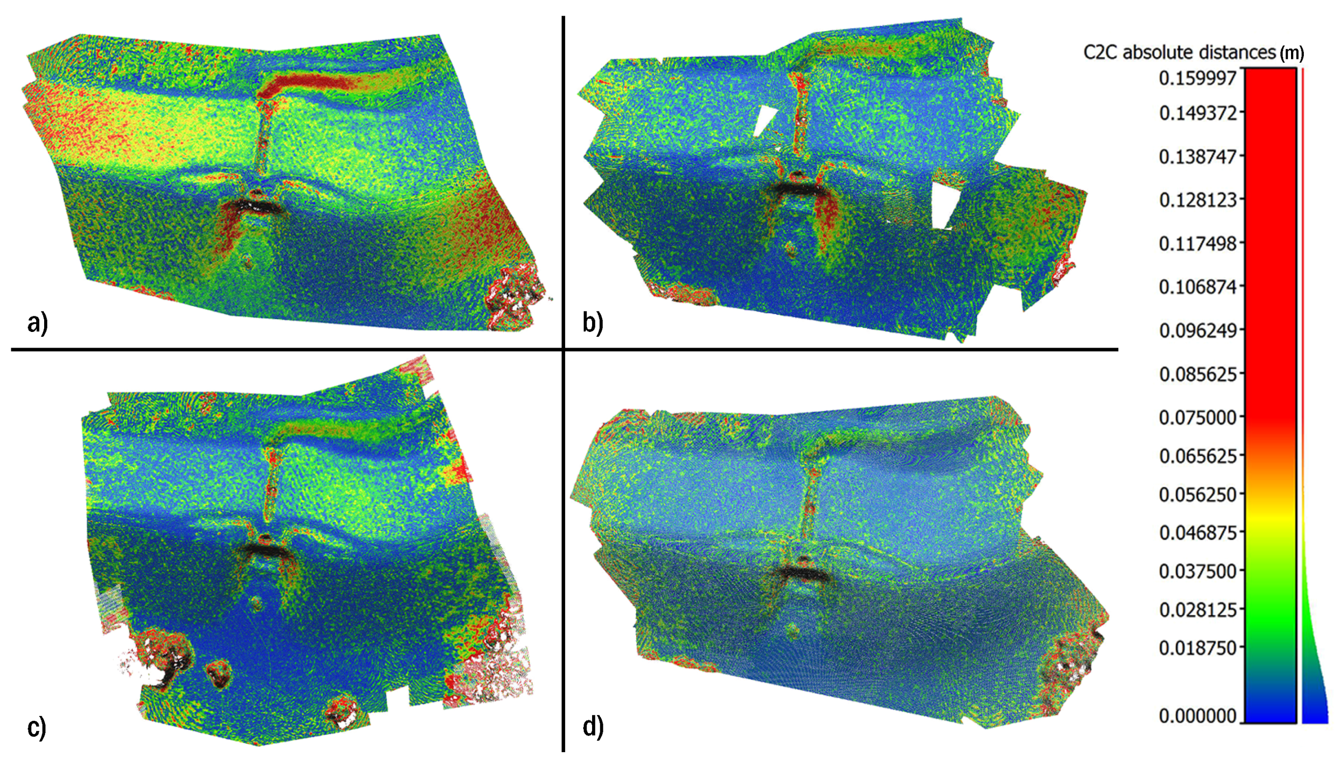
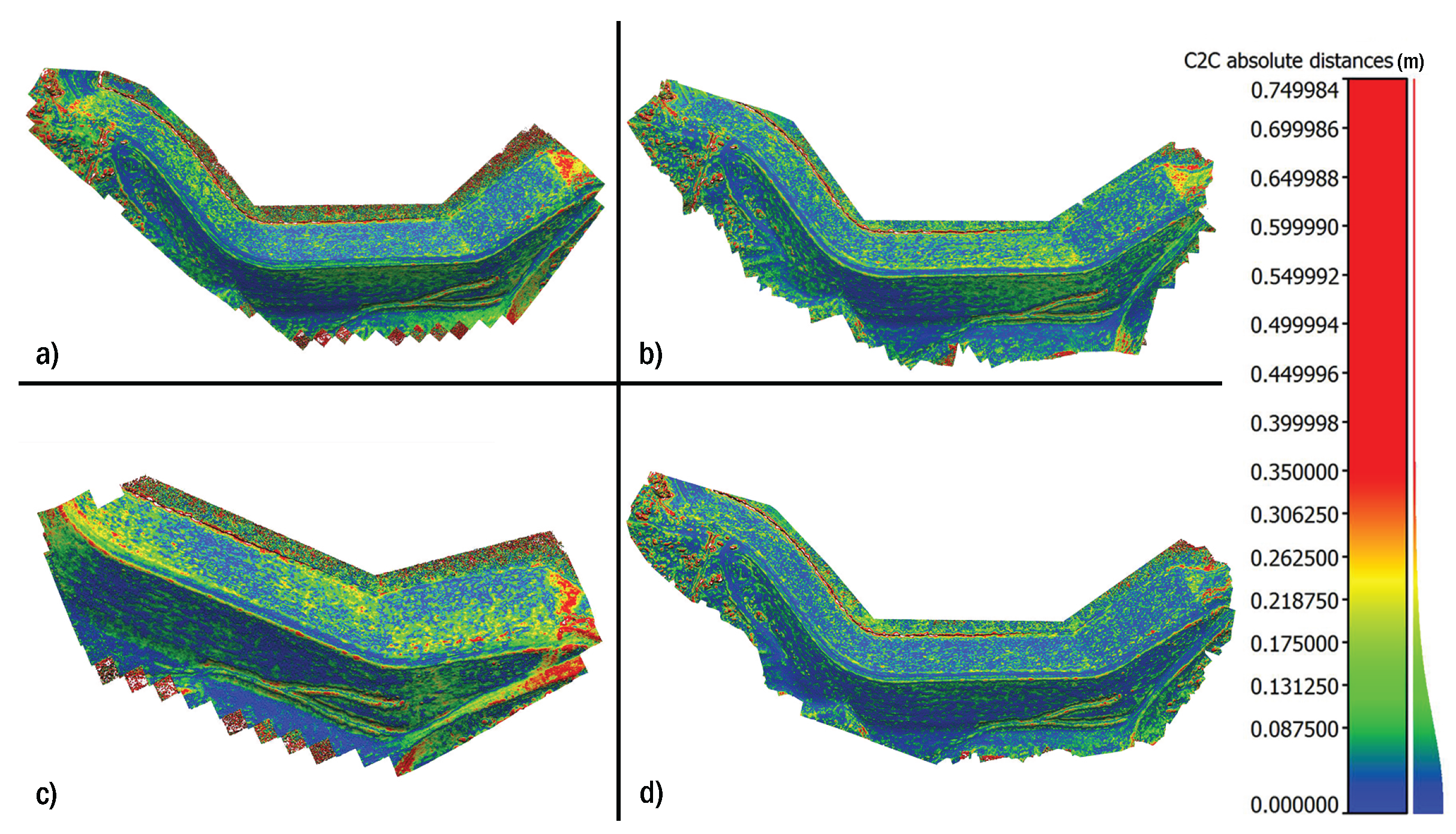
From the results shown, it can be seen that the optimized view planner succeeds in meeting the objectives of increasing model accuracy and completeness. The average error decreased by 43% in the first case and 23% in the second case when compared to the basic grid survey. The standard deviation of the error is also decreased significantly, by 29% in Case 1 and 19% in Case 2, and model completeness is improved in both cases. The optimized solution also compares favorably with the other two alternative flight paths. The increase in accuracy obtained by simply perturbing the grid solution is a particularly interesting result and potentially indicates a simple way to achieve meaningful increases in accuracy during surveying. The increase in accuracy in both this and the optimized case can most likely be attributed to the additional viewing angles provided, which increases the geometric strength of the photogrammetric network. Note that the results of the optimized view plan in the small case study are comparable to those obtained by Hoppe et al. in their physical survey of a site of similar size, where an accuracy of 5 cm was achieved over 92% of the desired points [38].

The tested arc pattern seems to provide inconsistent results, with good performance in the first case and poor performance in the second. The lack of coverage achieved by the arc pattern in the second test case is surprising, as intuitively adding additional images should improve performance, not reduce it. The authors are unsure of the meaning of this result. It is possible that this flight path is not well suited to long rectangular sites or perhaps some error was made in this portion of the experiment.

It should also be noted that the simulations have yet to be validated through physical flight tests, and it is expected that the physical error values will decrease appreciably from the simulated error due to the additional detail available for feature matching in real-world images. However, it is expected that the degree of improvement between the grid and optimized view plans will be similar to the simulated case. Another important note in transitioning to physical tests is the possibility of systematic error in the results due to self-calibration of the camera parameters during reconstruction. This issue is described in detail by James and Robson [66]. The minimal systematic error observed in the current results may be due to reduced sub-pixel effects in the simulated environment used. This leads to less noise in feature matching, which can improve the performance of the auto-calibrating bundle adjustment and result in less systematic error. While not greatly impacting the current work, the effects described by James and Robson will be an important aspect in evaluating the results of future work in real environments.

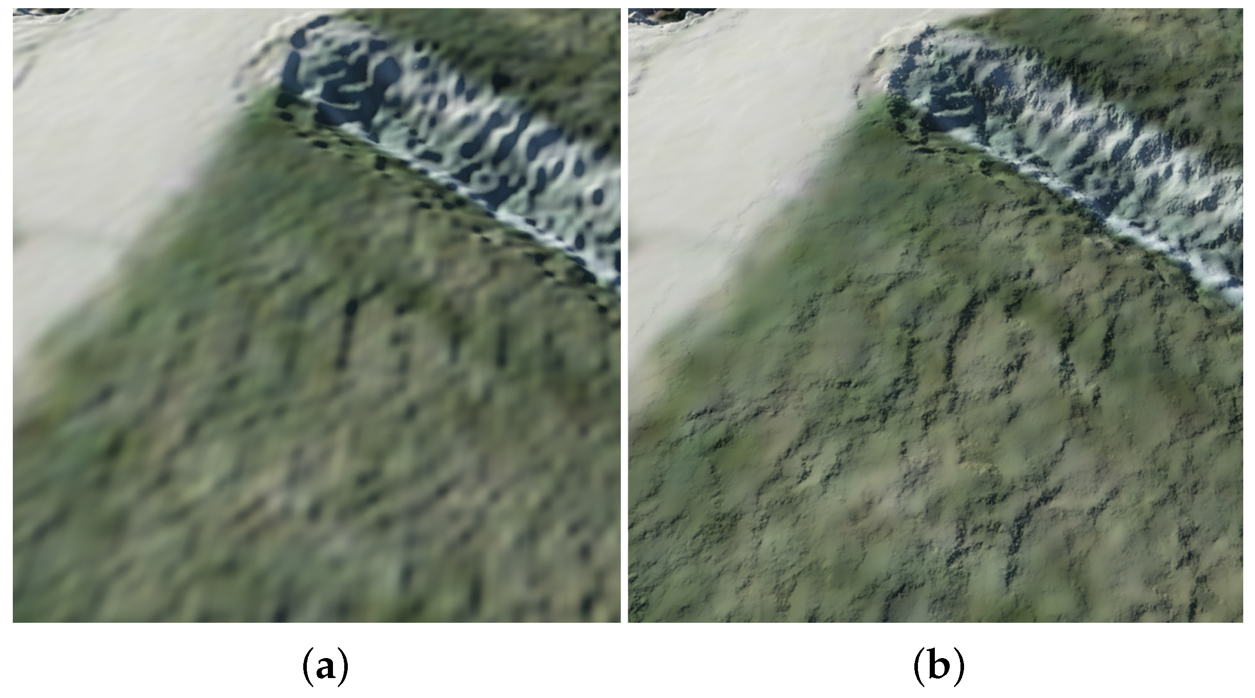
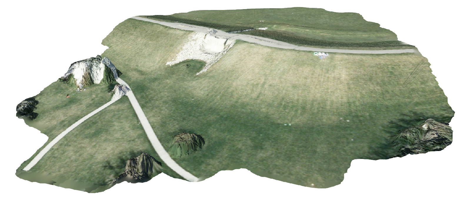
As stated above, it is probable that the simulation environment itself has some effect on the results produced, and this will be explored further in future work. It is readily apparent that the simulation does not reproduce fine surface details, such as grass and gravel, with a high degree of fidelity, and this is the reason the artificial surface roughness was introduced. The exact effect of this situation is less clear. Because of the close range, the resolution of the rendered imagery is higher than the draped imagery, meaning that a large amount of interpolation is occurring. Some areas of the orthoimagery, such as the rocks in the spillway, have large texture variations and provide sufficient features for matching. Other areas, such as the grass next to the spillway, are largely homogeneous, and the feature matching depends almost entirely on the artificial detail, which could potentially impact the accuracy of these areas. This is a larger issue in the first simulation than in the second, where higher resolution elevation data and imagery were used. These sites were chosen not only for the simulations in the current work, but also as sites for flight tests in future work. The authors plan not only to validate the optimized flight paths in future tests, but also to explore the relationship between results in the simulated environment and those from the physical sites. The large variety of features and surfaces at these sites should provide an instructive comparison and bring to light any surface effects masked by the simulator.

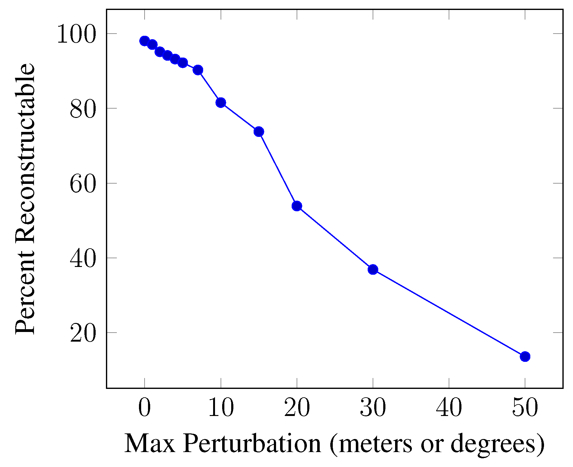
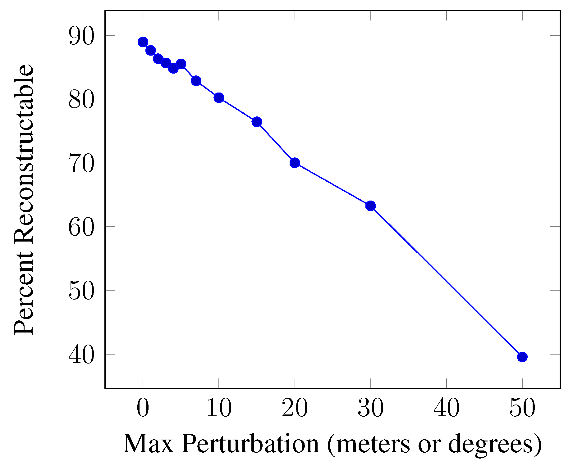
It is noted that the predicted percentages of terrain reconstruction are lower than the percentages reconstructed in the simulations, particularly for the grid surveys. There are several possible explanations for this discrepancy. The first is that the camera model used for planning and scoring in MATLAB does not perfectly represent the actual camera. In particular, the maximum camera range for each case is set to ensure a minimum GSD of 1 cm. This means that any terrain points beyond the maximum range are considered invisible by the camera. This is helpful in driving the optimized solution towards the minimum sampling distance, but could potentially underestimate the number of visible terrain points, as points beyond the maximum range are still actually visible, just at a larger GSD. This effect may be particularly pronounced in the grid survey, as all of the camera locations are on a flat plane, and the terrain is not flat.

A second possible reason for the low percent reconstructable values is that the name percent reconstructable may be something of a misnomer. It would be more accurate to say that the metric represents the percentage of terrain points that are visible from at least three camera locations at three distinct angles. The metric was intended to represent the minimum criteria for a point to be reconstructed using structure from motion, but does not fully capture the dense stereo pair matching used in multi-view stereo. Because Photoscan uses both techniques in its reconstruction pipeline, the percent reconstructable metric does not always represent all of the areas reconstructed in the final model.

Despite these shortcomings, the percent reconstructable metric (while not a perfect reflection of the final level of model reconstruction) does appear to trend generally with the final model accuracy and, thus, is helpful in motivating the genetic algorithm towards more accurate solutions.

5. Conclusions

This work presented a genetic algorithm-based view planner for UAV terrain modeling. The algorithm used structure from motion reconstruction criteria to guide the selection of viewpoints for images taken during a UAV mission. Rough terrain data were imported from public data sources or prior missions and used as an outline of the terrain geometry for view planning purposes. A novel simulation environment was developed using high fidelity terrain generation software to facilitate quantifiable and repeatable view plan testing and comparison.

The performance of the view planning algorithm is tested in both large- and small-scale infrastructure case studies. The performance of the algorithm is evaluated against three alternative plans, a traditional grid pattern, a grid with added noise and a grid with added arcs. The algorithm produces optimized flight paths that increased the accuracy of reconstructed models by up to 43% versus the basic grid. Increases in model completeness are also observed in the optimized paths.

Although the results of the current study are favorable, much work remains to be done. Future studies will conduct physical flight tests to validate both the presented simulation environment and the computed view plans. Work must be done to establish the correlation between the accuracy obtained through simulation and that obtained in experiment. The genetic algorithm implemented, while capable of producing quality results, is a stochastic tool and, thus, cannot guarantee an optimum solution. It is possible that seeding the algorithm with additional heuristic solutions will improve the consistency of the results obtained, and this will be explored in future work. The tradeoffs between flight time, accuracy and model completeness in optimal view planning also require additional study. Real-time and onboard view planning should also be explored to account for imperfect platform positioning and changing flight conditions throughout the mission.

References

1. Watts, A.C.; Ambrosia, V.G.; Hinkley, E.A. Unmanned aircraft systems in remote sensing and scientific research: Classification and considerations of use. Remote Sens. 2012, 4, 1671–1692. [Google Scholar] [CrossRef]
2. Walsh, J.I. The Effectiveness of Drone Strikes in Counterinsurgency and Counterterrorism Campaigns. Available online: http://www.strategicstudiesinstitute.army.mil/pubs/display.cfm?pubID=1167 (accessed on 30 December 2015).
3. Lelong, C.C.D. Assessment of unmanned aerial vehicles imagery for quantitative monitoring of wheat crop in small plots. Sensors 2008, 8, 3557–3585. [Google Scholar] [CrossRef]
4. Lucieer, A.; Jong, S.M.D.; Turner, D. Mapping landslide displacements using Structure from Motion (SfM) and image correlation of multi-temporal UAV photography. Prog. Phys. Geogr. 2013, 38, 97–116. [Google Scholar] [CrossRef]
5. Hausamann, D.; Zirnig, W.; Schreier, G.; Strobl, P. Monitoring of gas pipelines, a civil UAV application. Aircr. Eng. Aerosp. Technol. 2005, 77, 352–360. [Google Scholar] [CrossRef]
6. Irschara, A.; Kaufmann, V.; Klopschitz, M.; Bischof, H.; Leberl, F. Towards fully automatic photogrammetric reconstruction using digital images taken from UAVs. In Proceedings of the International Society for Photogrammetry and Remote Sensing Symposium, 100 Years ISPRS - Advancing Remote Sensing Science, Vienna, Austria, 5–7 July 2010; pp. 65–70.
7. Zhang, C.; Elaksher, A. An unmanned aerial vehicle-based imaging system for 3D measurement of unpaved road surface distresses1. Comput. Aided Civil Infrastruct. Eng. 2012, 27, 118–129. [Google Scholar] [CrossRef]
8. Tong, X.; Liu, X.; Chen, P.; Liu, S.; Luan, K.; Li, L.; Liu, S.; Liu, X.; Xie, H.; Jin, Y.; et al. Integration of UAV-based photogrammetry and terrestrial laser scanning for the three-dimensional mapping and monitoring of open-pit mine areas. Remote Sens. 2015, 7, 6635–6662. [Google Scholar] [CrossRef]
9. Mathews, A.J.; Jensen, J.L.R. Visualizing and quantifying vineyard canopy LAI using an unmanned aerial vehicle (UAV) collected high density structure from motion point cloud. Remote Sens. 2013, 5, 2164–2183. [Google Scholar] [CrossRef]
10. Koenderink, J.J.; van Doorn, A.J. Affine structure from motion. JOSA A 1991, 8, 377–385. [Google Scholar] [CrossRef]
11. Niethammer, U.; James, M.; Rothmund, S.; Travelletti, J.; Joswig, M. UAV-based remote sensing of the Super-Sauze landslide: Evaluation and results. Eng. Geol. 2012, 128, 2–11. [Google Scholar] [CrossRef]
12. Bosché, F.; Halatsch, J.; Jahanshahi, M.R.; Masri, S.F. Adaptive vision-based crack detection using 3D scene reconstruction for condition assessment of structures. Autom. Constr. 2012, 22, 567–576. [Google Scholar]
13. James, M.R.; Robson, S. Straightforward reconstruction of 3D surfaces and topography with a camera: Accuracy and geoscience application. J. Geophys. Res. 2012, 117, F03017. [Google Scholar] [CrossRef]
14. Schmid, K.; Hirschmüller, H.; Dömel, A.; Grixa, I.; Suppa, M.; Hirzinger, G. View planning for multi-view stereo 3D Reconstruction using an autonomous multicopter. J. Intell. Robot. Syst. Theory Appl. 2012, 65, 309–323. [Google Scholar] [CrossRef]
15. Chen, S.; Li, Y.; Kwok, N.M. Active vision in robotic systems: A survey of recent developments. Int. J. Robot. Res. 2011, 30, 1343–1377. [Google Scholar] [CrossRef]
16. Zhao, J.; Cheung, S.C.S. Optimal visual sensor planning. In Proceedings of the IEEE International Symposium on Circuits and Systems, Taipei, Taiwan, 24–27 May 2009; pp. 165–168.
17. Chen, S.Y.; Li, Y.F. Automatic sensor placement for model-based robot vision. IEEE Trans. Syst. Man Cybern. Part B Cybern. 2004, 34, 393–408. [Google Scholar] [CrossRef]
18. Remagnino, P.; Illingworth, J.; Kittler, J.; Matas, J. Intentional control of camera look direction and viewpoint in an active vision system. Image Vis. Comput. 1995, 13, 79–88. [Google Scholar] [CrossRef]
19. Kristensen, S. Sensor planning with Bayesian decision theory. Robot. Auton. Syst. 1997, 19, 273–286. [Google Scholar] [CrossRef]
20. Dunn, E.; Frahm, J.M. Next best view planning for active model improvement. In Proceedings of the British Machine Vision Conference, London, UK, 7–10 September 2009; pp. 53.1–53.11.
21. Krainin, M.; Curless, B.; Fox, D. Autonomous generation of complete 3D object models using next best view manipulation planning. In Proceedings of the IEEE International Conference on Robotics and Automation, Shanghai, China, 9–13 May 2011; pp. 5031–5037.
22. Trummer, M.; Munkelt, C.; Denzler, J. Online next-best-view planning for accuracy optimization using an extended E-criterion. In Proceedings of the International Conference on Pattern Recognition, Istanbul, Turkey, 23–26 August 2010; pp. 1642–1645.
23. Wenhardt, S.; Deutsch, B.; Angelopoulou, E.; Niemann, H. Active visual object reconstruction using D-, E-, and T-optimal next best views. In Proceedings of the IEEE Conference on Computer Vision and Pattern Recognition, 2007, CVPR’07. Minneapolis, MN, USA, 17–22 June 2007; pp. 1–7.
24. Scott, W.R.; Roth, G.; Rivest, J.F. View Planning with a Registration Constraint. Proc. 3rd Int. Conf. 3D Digit. Imaging Model. 2001, 127–134. [Google Scholar] [CrossRef]
25. Cowan, C.K.; Kovesi, P.D. Automatic sensor placement from vision task requirements. IEEE Trans. Pattern Anal. Mach. Intell. 1988, 10, 407–415. [Google Scholar] [CrossRef]
26. Tarbox, G.; Gottschlich, S. Planning for complete sensor coverage in inspection. Comput. Vis. Image Underst. 1995, 61, 84–111. [Google Scholar] [CrossRef]
27. Tarabanis, K.A.; Tsai, R.Y.; Allen, P.K. MVP sensor planning system for robotic vision tasks. IEEE Trans. Robot. Autom. 1995, 11, 72–85. [Google Scholar] [CrossRef]
28. Chen, S.; Li, Y.F.; Zhang, J.; Wang, W. Active sensor planning for multiview vision tasks. Springer: Berlin/Heidelberg, Germany, 2008; pp. 1–265. [Google Scholar]
29. Current, J.R.; Schilling, D.A. The covering salesman problem. Transp. Sci. 1989, 23, 208–213. [Google Scholar] [CrossRef]
30. Scott, W.R.; Roth, G.; Rivest, J.F. View planning for automated three-dimensional object reconstruction and inspection. ACM Comput. Surv. 2003, 35, 64–96. [Google Scholar] [CrossRef]
31. Van Leeuwen, J.; Leeuwen, J. Handbook of Theoretical Computer Science: Algorithms and complexity; Handbook of Theoretical Computer Science, Elsevier: Amsterdam, The Netherlands, 1994. [Google Scholar]
32. Scott, W.R. Model-based view planning. Mach. Vis. Appl. 2007, 20, 47–69. [Google Scholar] [CrossRef]
33. Blaer, P.; Allen, P. Data acquisition and view planning for 3-D modeling tasks. In Proceedings of the IEEE/RSJ International Conference on Intelligent Robots and Systems, 2007, IROS 2007. San Diego, CA, USA, 29 October – 2 November 2007; pp. 417–422.
34. Ali Hosseininaveh, A.; Sargeant, B.; Erfani, T.; Robson, S.; Shortis, M.; Hess, M.; Boehm, J. Towards fully automatic reliable 3D acquisition: From designing imaging network to a complete and accurate point cloud. Robot. Auton. Syst. 2014, 62, 1197–1207. [Google Scholar] [CrossRef]
35. Alsadik, B.; Gerke, M.; Vosselman, G.; Daham, A.; Jasim, L. Minimal camera networks for 3D image based modeling of cultural heritage objects. Sensors (Basel, Switzerland) 2014, 14, 5785–804. [Google Scholar] [CrossRef] [PubMed]
36. Blaer, P.; Allen, P. Two stage view planning for large-scale site modeling. In Proceedings of the Third International Symposium on 3D Data Processing, Visualization, and Transmission, Chapel Hill, NC, USA, 14–16 June 2006; pp. 814–821.
37. Blaer, P.; Allen, P. View planning for automated site modeling. In Proceedings of the 2006 IEEE International Conference on Robotics and Automation, ICRA 2006. Orlando, FL, USA, 15–19 May 2006; pp. 2621–2626.
38. Hoppe, C.; Wendel, A.; Zollmann, S.; Pirker, K.; Irschara, A.; Bischof, H.; Kluckner, S. Photogrammetric camera network design for micro aerial vehicles. Comput. Vis. Winter Workshop (CVWW) 2012, 8, 1–3. [Google Scholar]
39. Englot, B.; Hover, F. Planning complex inspection tasks using redundant roadmaps. Proc. Int. Symp. Robot. Res 2011, 8, 1–16. [Google Scholar]
40. Hollinger, G.A.; Englot, B.; Hover, F.; Mitra, U.; Sukhatme, G.S. Uncertainty-driven view planning for underwater inspection. In Proceedings of the IEEE International Conference on Robotics and Automation, Saint Paul, MN, USA, 14–18 May 2012; pp. 4884–4891.
41. Olague, G. Autonomous photogrammetric network design using genetic algorithms. Appl. Evolut. Comput. 2001, 2037, 353–363. [Google Scholar]
42. Christofides, N. Worst-Case Analysis of A New Heuristic for the Travelling Salesman Problem; Management Sciences Research Report; Defense Technical Information Center: Belvoir, VA, USA, 1976. [Google Scholar]
43. Yang, G.; Dong, R.; Wu, H.; Liu, C. Viewpoint optimization using genetic algorithm for flying robot inspection of electricity transmission tower equipment. Chin. J. Electron. 2014, 23, 426–431. [Google Scholar]
44. Remondino, F.; Barazzetti, L.; Nex, F.; Scaioni, M.; Sarazzi, D. UAV photgrammetry for mapping and 3D modeling, current status and future perspectives. In Proceedings of the International Archives of the Photogrammetry, Remote Sensing and Spatial Information Sciences, Zurich, Switzerland, 4–16 September 2011; pp. 14–16.
45. Gantovnik, V.B.; Anderson-Cook, C.M.; Gürdal, Z.; Watson, L.T. A genetic algorithm with memory for mixed discrete continuous design optimization. Comput. Struct. 2003, 81, 2003–2009. [Google Scholar] [CrossRef]
46. Mitchell, M. An Introduction to Genetic Algorithms; Complex Adaptive Systems, MIT Press: Cambridge, MA, USA, 1998. [Google Scholar]
47. Dollison, R.M. The National Map: New viewer, services, and data download: U.S. Geological Survey Fact Sheet 2010–3055. Available online: http://pubs.er.usgs.gov/publication/fs20103055 (accessed on 25 December 2015).
48. Eisenbeiss, H.; Grün, A. UAV Photogrammetry. Ph.D Thesis, Institute of Photogrammetry and Remote Sensing, Timmins, ON, Canada, 2009. [Google Scholar]
49. Haala, N.; Cramer, M.; Rothermel, M. Quality of 3D point clouds from highly overlapping uav imagery. Int. Arch. Photogramm. Remote Sens. Spat. Inf. Sci. 2013, XL, 4–6. [Google Scholar] [CrossRef]
50. Stoermer, J. DroneMapper Aerial Imagery and UAV Mapping “Best Practice” Guidelines. Available online: http://diydrones.com/profiles/blogs/dronemapper-aerial-imagery-and-uav-mapping-best-practice (accessed on 14 December 2015).
51. DroneMapper. Aerial Data Collection Guidelines & Flight Planning. Available online: https://conservationdrones.files.wordpress.com/2013/01/dronemapper_aerialdatacollectionguidelinesplanning.pdf (accessed on 3 December 2015).
52. Pix4D. Designing the Images Acquisition Plan. Available online: https://support.pix4d.com/hc/en-us/articles/202557459. (accessed on 3 December 2015).
53. Černý, V. Thermodynamical approach to the traveling salesman problem: An efficient simulation algorithm. J. Optim. Theory Appl. 1985, 45, 41–51. [Google Scholar] [CrossRef]
54. Potvin, J. Genetic algorithms for the traveling salesman problem. Ann. Oper. Res. 1996, 63, 337–370. [Google Scholar] [CrossRef]
55. Rosenkrantz, D.; Stearns, R.; Lewis Philip, M.I. An Analysis of Several Heuristics for Thetraveling Salesman Problem. In Fundamental Problems in Computing; Ravi, S., Shukla, S., Eds.; Springer Netherlands: Dordrecht, The Netherlands, 2009; pp. 45–69. [Google Scholar]
56. Gutin, G.; Punnen, A. The Traveling Salesman Problem and its Variations; Springer: New York, NY, USA, 2007. [Google Scholar]
57. Cloud Compare (version 2.6)[GPL software]. Available online: http://www.danielgm.net/cc (accessed on 30 December 2015).
58. Besl, P.; McKay, N.D. A method for registration of 3-D shapes. Pattern Anal. Mach. Intell. IEEE Trans. 1992, 14, 239–256. [Google Scholar] [CrossRef]
59. Kazhdan, M.; Bolitho, M.; Hoppe, H. Poisson surface reconstruction. In Proceedings of the Fourth Eurographics Symposium on Geometry Processing, Sardinia, Italy, 26–28 June 2006; Volume 7.
60. Wang, K.L.; Huang, Z.J.; Lin, J.T. Reinvestigation and analysis a landslide dam event in 2012 using UAV. EGU General Assem. 2015 2015, 17, 14035. [Google Scholar]
61. Liu, P.; Chen, A.Y.; Huang, Y.N.; Han, J.Y.; Lai, J.S. A review of rotorcraft Unmanned Aerial Vehicle (UAV) developments and applications in civil engineering. Smart Struct. Syst. 2014, 13, 1065–1094. [Google Scholar] [CrossRef]
62. Rathinam, S.; Kim, Z.W.; Sengupta, R. Vision-based monitoring of locally linear structures using an unmanned aerial vehicle1. J. Infrastruct. Syst. 2008, 14, 52–63. [Google Scholar] [CrossRef]
63. Zhang, C. An UAV-based photogrammetric mapping system for road condition assessment. Int. Arch. Photogramm. Remote Sens. Spat. Inf. Sci. 2008, 37, 627–632. [Google Scholar]
64. Walter, M.; Niethammer, U.; Rothmund, S.; Joswing, M. Joint analysis of the Super-Sauze (French Alps) mudslide by nanoseismic monitoring and UAV-based remote sensing. First Break 2009, 27, 75–82. [Google Scholar]
65. Nikolic, J.; Burri, M.; Rehder, J.; Leutenegger, S.; Huerzeler, C.; Siegwart, R. A UAV system for inspection of industrial facilities. In Proceedings of the Aerospace Conference, 2013 IEEE, Big Sky, MT, USA, 2–9 March 2013; pp. 1–8.
66. James, M.R.; Robson, S. Mitigating systematic error in topographic models derived from UAV and ground-based image networks. Earth Surf. Process. Landf. 2014, 39, 1413–1420. [Google Scholar] [CrossRef]
67. Agisoft, L. Agisoft PhotoScan User Manual; Professional Edition: New York, NY, USA, 2013. [Google Scholar]