
Remote Sensing Based Simple Models of GPP in Both Disturbed and Undisturbed Piñon-Juniper Woodlands in the Southwestern U.S.

Abstract
:
1. Introduction
2. Experimental Section
2.1. Site Description
2.2. Data
2.2.1. Gross Primary Productivity
2.2.2. Landsat ETM+
2.2.3. RapidEye

2.2.4. Spectral Vegetation Indices

| Model | VI Combination | Scale (m) |
|---|---|---|
| NDVILS | Landsat NDVI | 30 |
| NDVILSW | Landsat NDVI, NDWI | 30 |
| NDVIRE | RapidEye NDVI | 5 |
| NDVIREW | RapidEye NDVI, NDWI | 5, 30 |
| NDRE | RapidEye NDRE | 5 |
| NDREW | RapidEye NDRE, NDWI | 5, 30 |
2.3. Statistical Analysis
3. Results and Discussion
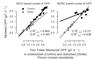
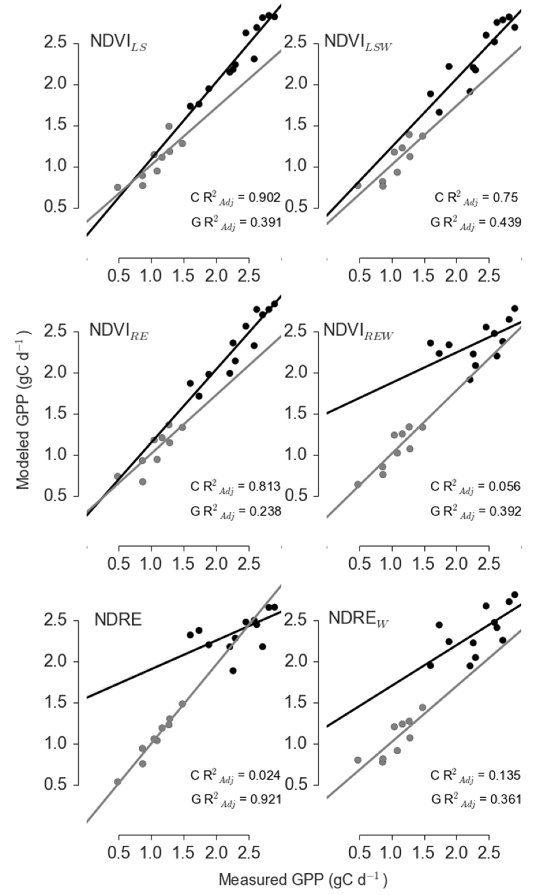
3.1. Models of GPP in PJ Woodlands Had the Lowest Error at the Disturbed Site
| Site | Sensor | Model | R2adj | ΔAICc | RelLL | Weights |
|---|---|---|---|---|---|---|
| Control | Landsat | NDVILS | 0.902 | 0 | 1 | 0.997 |
| Landsat | NDVILSW | 0.75 | 12.159 | 0.002 | 0.002 | |
| RapidEye | NDVIRE | 0.813 | 14.072 | 0.001 | 0.001 | |
| RapidEye | NDVIREW | 0.056 | 29.427 | 0 | 0 | |
| RapidEye | NDRE | 0.024 | 29.86 | 0 | 0 | |
| RapidEye | NDREW | 0.135 | 33.983 | 0 | 0 | |
| Girdle | Landsat | NDVILS | 0.391 | 18.428 | 0 | 0 |
| Landsat | NDVILSW | 0.439 | 17.684 | 0 | 0 | |
| RapidEye | NDVIRE | 0.238 | 41.847 | 0 | 0 | |
| RapidEye | NDVIREW | 0.392 | 39.812 | 0 | 0 | |
| RapidEye | NDRE | 0.921 | 0 | 1 | 1 | |
| RapidEye | NDREW | 0.361 | 18.851 | 0 | 0 |

| Site | Sensor | Model | R2adj | ΔAICc | RelLL | Weights |
|---|---|---|---|---|---|---|
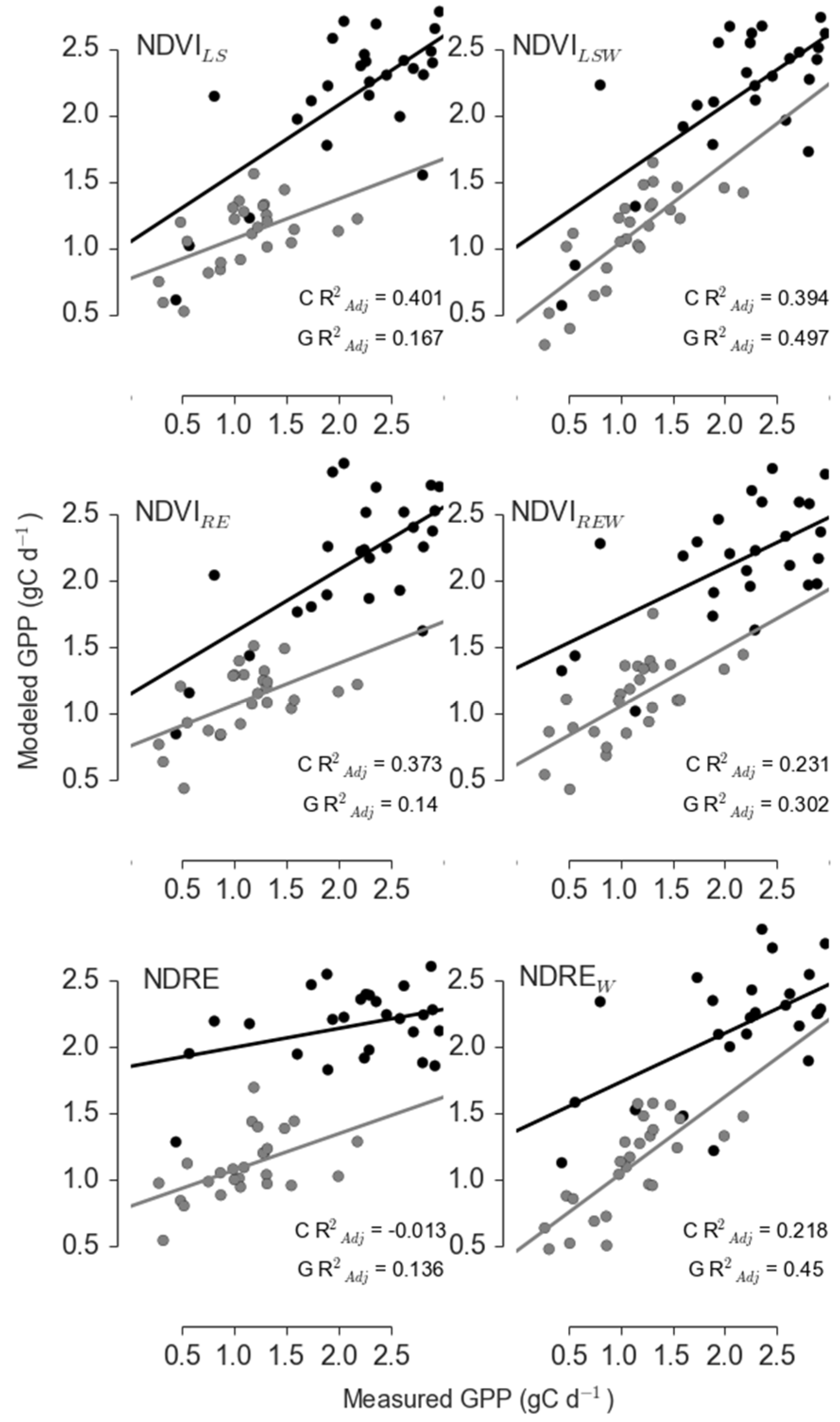
| Control | Landsat | NDVILS | 0.401 | 0.836 | 0.658 | 0.352 |
| Landsat | NDVILSW | 0.394 | 3.518 | 0.172 | 0.092 | |
| RapidEye | NDVIRE | 0.373 | 0 | 1 | 0.534 | |
| RapidEye | NDVIREW | 0.231 | 7.608 | 0.022 | 0.012 | |
| RapidEye | NDRE | −0.013 | 12.934 | 0.002 | 0.001 | |
| RapidEye | NDREW | 0.218 | 8.042 | 0.018 | 0.01 | |
| Girdle | Landsat | NDVILS | 0.167 | 10.991 | 0.004 | 0.004 |
| Landsat | NDVILSW | 0.497 | 0 | 1 | 0.899 | |
| RapidEye | NDVIRE | 0.14 | 13.979 | 0.001 | 0.001 | |
| RapidEye | NDVIREW | 0.302 | 8.552 | 0.014 | 0.012 | |
| RapidEye | NDRE | 0.136 | 11.945 | 0.003 | 0.002 | |
| RapidEye | NDREW | 0.45 | 4.803 | 0.091 | 0.081 |

3.2. NDRE and NDWI Reduced Model Error only during Periods of Significant Stress
| Site | Sensor | Model | R2adj | ΔAICc | RelLL | Weights |
|---|---|---|---|---|---|---|
| Control | Landsat | NDVILS | 0.815 | 0 | 1 | 0.899 |
| Landsat | NDVILSW | 0.698 | 4.414 | 0.11 | 0.099 | |
| RapidEye | NDVIRE | 0.795 | 22.327 | 0 | 0 | |
| RapidEye | NDVIREW | 0.292 | 12.08 | 0.002 | 0.002 | |
| RapidEye | NDRE | −0.042 | 15.56 | 0 | 0 | |
| RapidEye | NDREW | 0.5 | 30.359 | 0 | 0 | |
| Girdle | Landsat | NDVILS | 0.592 | 4.36 | 0.113 | 0.04 |
| Landsat | NDVILSW | 0.677 | 1.575 | 0.455 | 0.161 | |
| RapidEye | NDVIRE | 0.711 | 0.234 | 0.89 | 0.315 | |
| RapidEye | NDVIREW | 0.662 | 2.097 | 0.35 | 0.124 | |
| RapidEye | NDRE | 0.717 | 0 | 1 | 0.354 | |
| RapidEye | NDREW | 0.672 | 8.709 | 0.013 | 0.005 |
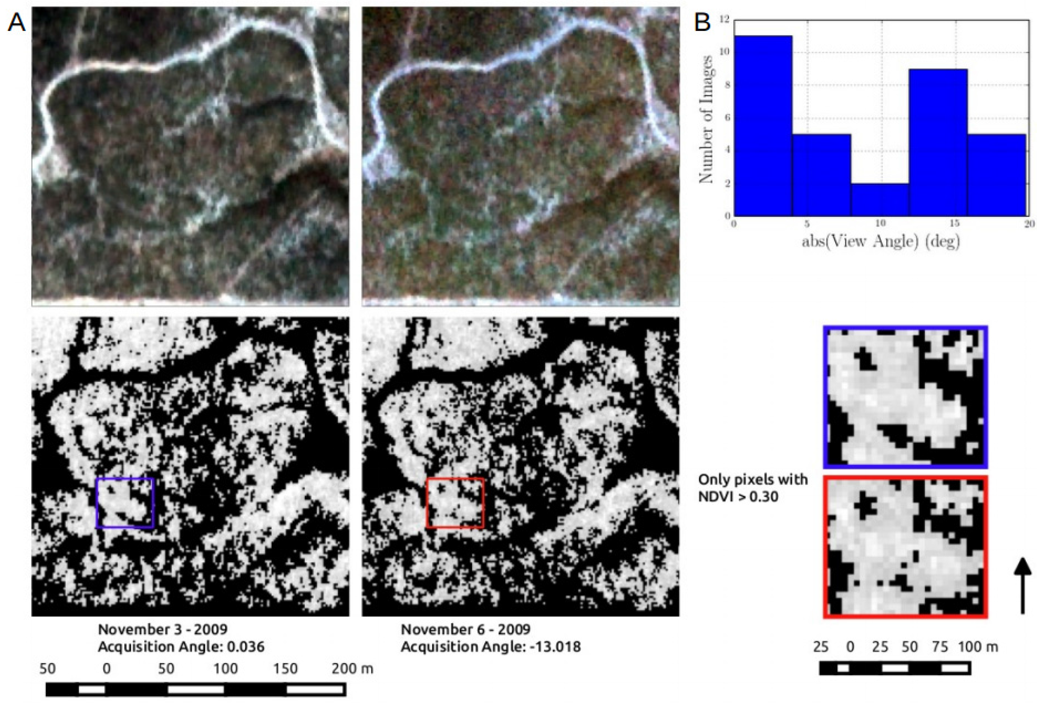
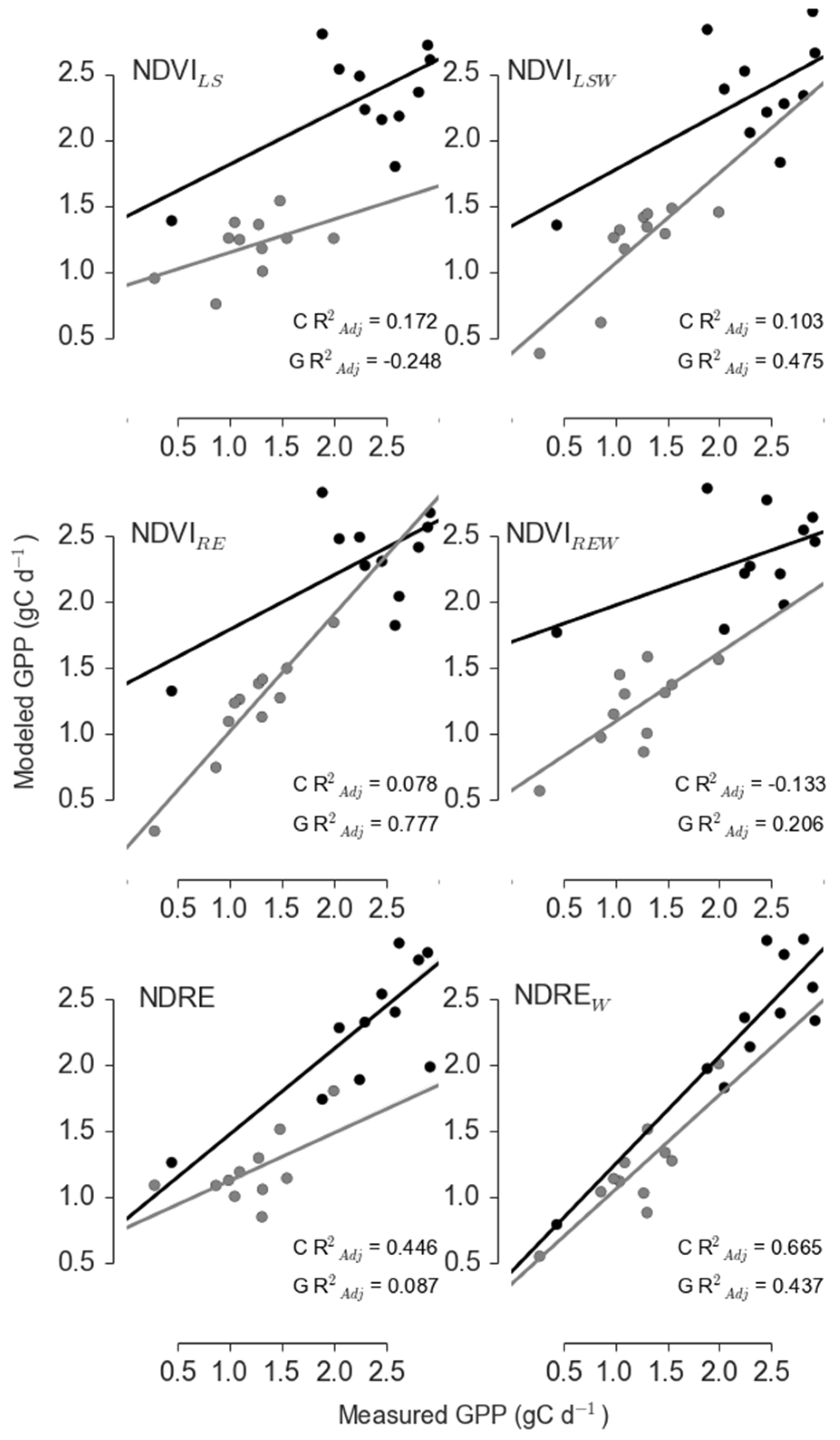
3.3. Inconsistency in Sensor View Imposed Significant Variability RapidEye VI Model Performance

| Site | Sensor | Model | R2adj | ΔAICc | RelLL | Weights |
|---|---|---|---|---|---|---|
| Control | Landsat | NDVILS | 0.172 | 0.134 | 0.935 | 0.348 |
| Landsat | NDVILSW | 0.103 | 5.782 | 0.056 | 0.021 | |
| RapidEye | NDVIRE | 0.078 | 6.113 | 0.047 | 0.018 | |
| RapidEye | NDVIREW | −0.133 | 8.584 | 0.014 | 0.005 | |
| RapidEye | NDRE | 0.446 | 0 | 1 | 0.372 | |
| RapidEye | NDREW | 0.665 | 0.91 | 0.634 | 0.236 | |
| Girdle | Landsat | NDVILS | −0.248 | 9.964 | 0.007 | 0.003 |
| Landsat | NDVILSW | 0.475 | 0.433 | 0.805 | 0.317 | |
| RapidEye | NDVIRE | 0.777 | 0 | 1 | 0.394 | |
| RapidEye | NDVIREW | 0.206 | 4.985 | 0.083 | 0.033 | |
| RapidEye | NDRE | 0.087 | 0.894 | 0.64 | 0.252 | |
| RapidEye | NDREW | 0.437 | 10.209 | 0.006 | 0.002 |

3.4. Implications for Regional Remote Sensing Based Estimations of GPP in PJ Woodlands
4. Conclusions
Acknowledgments
Author Contributions
Conflicts of Interest
References
- Poulter, B.; Frank, D.; Ciais, P.; Myneni, R.B.; Andela, N.; Bi, J.; Broquet, G.; Canadell, J.G.; Chevallier, F.; Liu, Y.Y.; et al. Contribution of semi-arid ecosystems to interannual variability of the global carbon cycle. Nature 2014, 509, 600–603. [Google Scholar] [CrossRef] [PubMed]
- Ahlstrom, A.; Raupach, M.R.; Schurgers, G.; Smith, B.; Arneth, A.; Jung, M.; Reichstein, M.; Canadell, J.G.; Friedlingstein, P.; Jain, A.K.; et al. The dominant role of semi-arid ecosystems in the trend and variability of the land CO2 sink. Science 2015, 348, 895–899. [Google Scholar] [CrossRef] [PubMed]
- Intergovernmental Panel on Climate Change (IPCC). Climate Change 2007: Impacts, Adaptation, and Vulnerability; Contribution of Working Group II to the Fourth Assessment Report of the Intergovernmental Panel on Climate Change; IPCC: Cambridge, UK, 2007. [Google Scholar]
- Seager, R.; Ting, M.; Held, I.; Kushnir, Y.; Lu, J.; Vecchi, G.; Huang, H.; Harnik, N.; Leetmaa, A.; Lau, N.; et al. Model projections of an imminent transition to a more arid climate in southwestern North America. Science 2007, 316, 1181–1184. [Google Scholar] [CrossRef] [PubMed]
- Seager, R.; Naik, N.; Vogel, L. Does global warming cause intensified interannual hydroclimate variability? J. Clim. 2012, 25, 3355–3372. [Google Scholar] [CrossRef]
- Intergovernmental Panel on Climate Change (IPCC). Climate Change 2014: Impacts, Adaptation, and Vulnerability. Part B: Regional Aspects. Contribution of Working Group II to the Fifth Assessment Report of the Intergovernmental Panel on Climate Change; Barros, V.R., Field, C.B., Dokken, D.J., Mastrandrea, M.D., Mach, K.J., Bilir, T.E., Chatterjee, M., Ebi, K.L., Estrada, Y.O., Genova, R.C., Eds.; Cambridge University Press: Cambridge, UK, 2014; p. 688. [Google Scholar]
- Garfin, G.; Franco, G.; Blanco, H.; Comrie, A.; Gonzalez, P.; Piechota, T.; Smyth, R.; Waskom, R. Southwest: Climate Change Impacts in the United States: The Third National Climate Assessment; Melillo, J.M., Richmond, T.C., Yohe, G.W., Eds.; USA Global Change Research Program: Washington, DC, USA, 2014; pp. 462–486. [Google Scholar]
- Allen, C.D.; Macalady, A.K.; Chenchouni, H.; Bachelet, D.; McDowell, N.; Vennetier, M.; Kitzberger, T.; Rigling, A.; Breshears, D.D.; Gonzalez, P.; et al. A global overview of drought and heat-induced tree mortality reveals emerging climate change risks for forests. For. Ecol. Manag. 2010, 259, 660–684. [Google Scholar] [CrossRef]
- Breshears, D.D.; Cobb, N.S.; Rich, P.M.; Price, K.P.; Allen, C.D.; Balice, R.G.; Romme, W.H.; Kastens, J.H.; Floyd, M.L.; Belnap, J.; et al. Regional vegetation die-off in response to global-change-type drought. Proc. Natl. Acad. Sci. USA 2005, 102, 15144–15148. [Google Scholar] [CrossRef] [PubMed]
- Clifford, M.; Royer, P.; Cobb, N. Precipitation thresholds and drought-induced tree die-off: Insights from patterns of Pinus edulis mortality along an environmental stress gradient. New Phytol. 2013, 200, 413–421. [Google Scholar] [CrossRef] [PubMed]
- Williams, A.; Allen, C.; Macalady, A. Temperature as a potent driver of regional forest drought stress and tree mortality. Nat. Clim. 2012, 3, 8–13. [Google Scholar] [CrossRef]
- Running, S.W.; Baldocchi, D.D.; Turner, D.P.; Gower, S.T.; Bakwin, P.S.; Hibbard, K.A. A global terrestrial monitoring network integrating tower fluxes, flask sampling, ecosystem modeling and eos satellite data. Remote Sens. Environ. 1999, 127, 108–127. [Google Scholar] [CrossRef]
- Zhao, M.; Running, S.; Heinsch, F.A. MODIS-derived terrestrial primary production. In Land Remote Sensing and Global Environmental Change; Ramachandran, B., Justice, C.O., Abrams, M.J., Eds.; Springer New York: New York, NY, USA, 2011; Volume 11, pp. 635–660. [Google Scholar]
- Monteith, J.L. Solar radiation and productivity in tropical ecosystems. J. Appl. Ecol. 1972, 9, 747–766. [Google Scholar] [CrossRef]
- Monteith, J.L.; Moss, C.J. Climate and the efficiency of crop production in britain and discussion. Philos. Trans. R. Soc. B Biol. Sci. 1977, 281, 277–294. [Google Scholar] [CrossRef]
- Tucker, C. Red and photographic infrared linear combinations for monitoring vegetation. Remote Sens. Environ. 1979, 8, 127–150. [Google Scholar] [CrossRef]
- Sims, D.; Rahman, A.; Cordova, V.; Elmasri, B.; Baldocchi, D.; Bolstad, P.; Flanagan, L.; Goldstein, A.; Hollinger, D.; Misson, L. A new model of gross primary productivity for North American ecosystems based solely on the enhanced vegetation index and land surface temperature from MODIS. Remote Sens. Environ. 2008, 112, 1633–1646. [Google Scholar] [CrossRef]
- Sims, D.A.; Brzostek, E.R.; Rahman, A.F.; Dragoni, D.; Phillips, R.P. An improved approach for remotely sensing water stress impacts on forest C uptake. Glob. Chang. Biol. 2014, 20, 2856–2866. [Google Scholar] [CrossRef] [PubMed]
- Yuan, W.; Liu, S.; Yu, G.; Bonnefond, J.-M.; Chen, J.; Davis, K.; Desai, R.R.; Goldstein, A.H.; Gianelle, D.; Rossi, F.; et al. Global estimates of evapotranspiration and gross primary production based on MODIS and global meteorology data. Remote Sens. Environ. 2010, 114, 1416–1431. [Google Scholar] [CrossRef]
- Verma, M.; Friedl, M.A.; Richardson, A.D.; Kiely, G.; Cescatti, A.; Law, B.E.; Wohlfahrt, G.; Gielen, B.; Roupsard, O.; Moors, E.J.; et al. Remote sensing of annual terrestrial gross primary productivity from MODIS: An assessment using the FLUXNET La Thuile data set. Biogeosciences 2014, 11, 2185–2200. [Google Scholar] [CrossRef] [Green Version]
- Fensholt, R.; Sandholt, I.; Rasmussen, M.S.; Stisen, S.; Diouf, A. Evaluation of satellite based primary production modeling in the semi-arid Sahel. Remote Sens. Environ. 2006, 105, 173–188. [Google Scholar] [CrossRef]
- Krofcheck, D.J.; Eitel, J.U.H.; Vierling, L.A.; Schulthess, U.; Hilton, T.M.; Dettweiler-Robinson, E.; Pendleton, R.; Litvak, M.E. Detecting mortality induced structural and functional changes in a piñon-juniper woodland using Landsat and RapidEye time series. Remote Sens. Environ. 2014, 151, 102–113. [Google Scholar] [CrossRef]
- Anderson-Teixeira, K.J.; Delong, J.P.; Fox, A.M.; Brese, D.A.; Litvak, M.E. Differential responses of production and respiration to temperature and moisture drive the carbon balance across a climatic gradient in New Mexico. Glob. Chang. Biol. 2011, 17, 410–424. [Google Scholar] [CrossRef]
- Huete, A.R.; Jackson, R.D.; Post, D.F. Spectral response of a plant canopy with different soil backgrounds. Remote Sens. Environ. 1985, 17, 37–53. [Google Scholar] [CrossRef]
- Huete, A.R. A soil-adjusted vegetation index (SAVI). Remote Sens. Environ. 1988, 25, 53–70. [Google Scholar] [CrossRef]
- Eitel, J.U.H.; Long, D.S.; Gessler, P.E.; Hunt, E.R.; Brown, D.J. Sensitivity of ground-based remote sensing estimates of wheat chlorophyll content to variation in soil reflectance. Soil Sci. Soc. Am. J. 2009, 73, 1715–1723. [Google Scholar] [CrossRef]
- Carter, G.A.; Knapp, A.K. Leaf optical properties in higher plants: Linking spectral characteristics to stress and chlorophyll concentration. Am. J. Bot. 2001, 88, 677–684. [Google Scholar] [CrossRef] [PubMed]
- Hendry, G.A.F.; Houghton, J.D.; Brown, S.B. The degradation of chlorophyll—A biological enigma. New Phytol. 1987, 107, 255–302. [Google Scholar] [CrossRef]
- Carter, G.A.; Miller, R.L. Early detection of plant stress by digital imaging within narrow stress-sensitive wavebands. Remote Sens. Environ. 1994, 50, 295–302. [Google Scholar] [CrossRef]
- Eitel, J.U.H.; Long, D.S.; Gessler, P.E.; Smith, A.M.S. Using in-situ measurements to evaluate the new RapidEye satellite series for prediction of wheat nitrogen status. Int. J. Remote Sens. 2007, 28, 4183–4190. [Google Scholar] [CrossRef]
- Eitel, J.U.H.; Long, D.S.; Gessler, P.E.; Hunt, E.R. Combined spectral index to improve ground-based estimates of nitrogen status in dryland wheat. Agron. J. 2008, 100, 1694–1702. [Google Scholar] [CrossRef]
- Eitel, J.U.H.; Keefe, R.F.; Long, D.S.; Davis, A.S.; Vierling, L.A. Active ground optical remote sensing for improved monitoring of seedling stress in nurseries. Sensors 2010, 10, 2843–2850. [Google Scholar] [CrossRef] [PubMed]
- Drought induced Tree Mortality and Ensuing Bark Beetle Outbreaks in Southwestern Pinyon-Juniper Woodlands. Available online: http://citeseerx.ist.psu.edu/viewdoc/download?doi=10.1.1.165.4291&rep=rep1&type=pdf#page=49 (accessed on 17 December 2015).
- Eitel, J.U.H.; Vierling, L.A.; Litvak, M.E.; Long, D.S.; Schulthess, U.; Ager, A.A.; Krofcheck, D.J.; Stoscheck, L. Broadband, red-edge information from satellites improves early stress detection in a New Mexico conifer woodland. Remote Sens. Environ. 2011, 115, 3640–3646. [Google Scholar] [CrossRef]
- Gitelson, A.A.; Merzlyak, M.N. Quantifying estimation of chlorophyll using reflectance spectra. J. Photochem. Photobiol. B Biol. 1994, 22, 247–252. [Google Scholar] [CrossRef]
- Webb, E.K.; Pearman, G.I.; Leuning, R. Correction of flux measurements for density effects due to heat and water vapour transfer. Quart. J. R. Met. Soc. 1980, 106, 85–100. [Google Scholar] [CrossRef]
- Massman, W.J. A simple method for estimating frequency response corrections for eddy covariance systems. Agric. For. Meteorol. 2000, 104, 185–198. [Google Scholar] [CrossRef]
- Lasslop, G.; Reichstein, M.; Papale, D.; Richardson, A.D.; Arneth, A.; Barr, A.; Stoy, P.; Wohlfahrt, G. Separation of net ecosystem exchange into assimilation and respiration using a light response curve approach: Critical issues and global evaluation. Glob. Chang. Biol. 2010, 16, 187–208. [Google Scholar] [CrossRef]
- Flanagan, L.; Wever, L.; Carlson, P. Seasonal and interannual variation in carbon dioxide exchange and carbon balance in a northern temperate grassland. Glob. Chang. Biol. 2002, 8, 599–615. [Google Scholar] [CrossRef]
- Hsieh, C.; Katul, G.; Chi, T. An approximate analytical model for footprint estimation of scalar fluxes in thermally stratified atmospheric flows. Adv. Water Resour. 2000, 23, 765–772. [Google Scholar] [CrossRef]
- Detto, M.; Montaldo, N.; Albertson, J.D.; Mancini, M.; Katul, G. Soil moisture and vegetation controls on evapotranspiration in a heterogeneous Mediterranean ecosystem on Sardinia, Italy. Water Resour. Res. 2006. [Google Scholar] [CrossRef]
- Roy, D.P.; Ju, J.; Kline, K.; Scaramuzza, P.L.; Kovalskyy, V.; Hansen, M.; Loveland, T.R.; Vermote, E.; Zhang, C. Web-enabled Landsat Data (WELD): Landsat ETM+ composited mosaics of the conterminous United States. Remote Sens. Environ. 2010, 114, 35–49. [Google Scholar] [CrossRef]
- Irish, R.I.; Barker, J.L.; Goward, S.N.; Arvidson, T. Characterization of the Landsat-7 ETM+ automated cloud-cover assessment (ACCA) algorithm. Photogramm. Eng. Remote Sens. 2006, 72, 1179–1188. [Google Scholar] [CrossRef]
- Hall, D.K.; Foster, J.L.; Verbyla, D.L.; Klein, A.G. Assessment of snow-cover mapping accuracy in a variety of vegetation-cover densities in central Alaska. Remote Sens. Environ. 1998, 66, 129–137. [Google Scholar] [CrossRef]
- Bedrick, E.J.; Tsai, C.L. Model selection for multivariate regression in small samples. Biometrics 1994, 50, 226–331. [Google Scholar] [CrossRef]
- Leuning, R.; Cleugh, H.A.; Zegelin, S.J.; Hughes, D. Carbon and water fluxes over a temperate Eucalyptus forest and a tropical wet/dry savanna in Australia: Measurements and comparison with MODIS remote sensing estimates. Agric. For. Meteorol. 2005, 129, 151–173. [Google Scholar] [CrossRef]
- Gu, Y.; Hunt, E.; Wardlow, B.; Basara, J.B.; Brown, J.F.; Verdin, J.P. Evaluation of MODIS NDVI and NDWI for vegetation drought monitoring using Oklahoma Mesonet soil moisture data. Geophys. Res. Lett. 2008, 35, 1–5. [Google Scholar] [CrossRef]
- Hunt, E.R.; Rock, B.N. Detection of changes in leaf water content using near- and middle-infrared reflectance. Remote Sens. Environ. 1989, 30, 43–54. [Google Scholar]
- Eitel, J.U.H.; Gessler, P.E.; Smith, A.M.S.; Robberecht, R. Suitability of existing and novel spectral indices to remotely detect water stress in Populus spp. For. Ecol. Manag. 2006, 229, 170–182. [Google Scholar] [CrossRef]
- Stoms, D.M.; Bueno, M.J.; Davis, F.W. Viewing geometry of AVHRR image composites derived using multiple criteria. Photogramm. Eng. Remote Sens. 1997, 63, 681–689. [Google Scholar]
- Abuzar, M.; Sheffield, K.; Whitfield, D.; O’Connell, M.; McAllister, A. Comparing inter-sensor NDVI for the analysis of horticulture crops in south-eastern Australia. Am. J. Remote Sens. 2014, 2, 1–9. [Google Scholar] [CrossRef]
- Stimson, H.C.; Breshears, D.D.; Ustin, S.L.; Kefauver, S.C. Spectral sensing of foliar water conditions in two co-occurring conifer species: Pinus edulis and Juniperus monosperma. Remote Sens. Environ. 2005, 96, 108–118. [Google Scholar] [CrossRef]
© 2015 by the authors; licensee MDPI, Basel, Switzerland. This article is an open access article distributed under the terms and conditions of the Creative Commons by Attribution (CC-BY) license (http://creativecommons.org/licenses/by/4.0/).
Share and Cite
Krofcheck, D.J.; Eitel, J.U.H.; Lippitt, C.D.; Vierling, L.A.; Schulthess, U.; Litvak, M.E. Remote Sensing Based Simple Models of GPP in Both Disturbed and Undisturbed Piñon-Juniper Woodlands in the Southwestern U.S. Remote Sens. 2016, 8, 20. https://doi.org/10.3390/rs8010020
Krofcheck DJ, Eitel JUH, Lippitt CD, Vierling LA, Schulthess U, Litvak ME. Remote Sensing Based Simple Models of GPP in Both Disturbed and Undisturbed Piñon-Juniper Woodlands in the Southwestern U.S. Remote Sensing. 2016; 8(1):20. https://doi.org/10.3390/rs8010020
Chicago/Turabian StyleKrofcheck, Dan J., Jan U. H. Eitel, Christopher D. Lippitt, Lee A. Vierling, Urs Schulthess, and Marcy E. Litvak. 2016. "Remote Sensing Based Simple Models of GPP in Both Disturbed and Undisturbed Piñon-Juniper Woodlands in the Southwestern U.S." Remote Sensing 8, no. 1: 20. https://doi.org/10.3390/rs8010020