Article

Assimilation of Two Variables Derived from Hyperspectral Data into the DSSAT-CERES Model for Grain Yield and Quality Estimation

1
Beijing Research Center for Information Technology in Agriculture, Beijing Academy of Agriculture and Forestry Sciences, Beijing 100097, China
2
National Engineering Research Center for Information Technology in Agriculture, Beijing 100097, China
3
Institute of Agricultural Remote Sensing and Information Application, Zhejiang University, Hangzhou 310029, China
4
Beijing Research Center for Agricultural Standards and Testing, Beijing Academy of Agriculture and Forestry Sciences, Beijing 100097, China
5
Key Laboratory for Information Technologies in Agriculture, The Ministry of Agriculture, Beijing 10097, China
6
Beijing Engineering Research Center of Agricultural Internet of Things, Beijing 100097, China
7
Key Laboratory of Wetland Ecology and Environment, Northeast Institute of Geography and Agroecology, Chinese Academy of Sciences, Changchun 130102, China
*
Author to whom correspondence should be addressed.
The author contributed equally to this work.
Remote Sens. 2015, 7(9), 12400-12418; https://doi.org/10.3390/rs70912400
Submission received: 29 June 2015 / Revised: 31 August 2015 / Accepted: 7 September 2015 / Published: 22 September 2015
(This article belongs to the Special Issue Remote Sensing in Precision Agriculture)

Abstract

:
The combination of remote sensing and crop growth models has become an effective tool for yield estimation and a potential method for grain quality estimation. In this study, two assimilation variables (derived from a hyperspectral sensor), called leaf area index (LAI) and canopy nitrogen accumulation (CNA), were jointly used to calibrate the sensitive parameters and initial states of the DSSAT-CERES crop model, to improve simulated output of the grain yield and protein content of winter wheat. The results show that the modified simple ratio (MSR) and normalized difference red edge (NDRE) better estimated LAI and CNA, respectively, compared with the other possible vegetation indices. The integration of both LAI and CNA resulted in a more robust DSSAT-CERES models with than each one alone. The R2 and RMSE values, respectively, of the regression between the simulated (using the two assimilation variables method) and measured LAI were 0.828 and 0.494, and for CNA were 0.808 and 20.26 kg N∙ha−1. These two assimilation variables resulted in grain yield and protein content estimates of winter wheat with a high precision and R2 and RMSE values of 0.698 and 0.726 ton∙ha−1, and 0.758% and 1.16%, respectively. This study provides a more robust method for estimating the grain yield and protein content of winter wheat based on the integration of the DSSAT-CERES crop model and remote sensing data.

Graphical Abstract

1. Introduction

Wheat (Triticum aestivum L.) is a staple food in North China, where the population accounts for about 40% of the country’s total [1,2]. The productivity of wheat, including grain yield and quality, directly determines its market price and related agriculture policies [3,4], and an advanced knowledge of grain yield and quality is important for this purpose [5,6]. The combination of remote sensing and crop growth simulation models has provided an effective tool for crop grain yield and quality estimation in regional studies [5,7].
Many studies have been focused on the integration of remote sensing and crop growth simulation models for crop growth monitoring and yield estimation [5,7,8]. Maas [9,10] initially described four techniques (input, updating, re-initialization, and re-parameterization) for leaf area indices (LAI) by incorporating remote sensing data into crop growth model estimations. Guerif and Duke [8,11] combined the Simple and Universal Crop Growth Simulator (SUCROS) model and the SAIL reflectance model to calibrate the site specific characteristics of soil and crops using remote sensing data, and they suggested that assimilation methods had a great potential for large-scale crop monitoring (e.g., yield prediction). Jongschaap [12] demonstrated simulation accuracy could be improved by run-time replacement for the Rotask simulation model with remote sensing observations. In a regional winter wheat and maize yield simulation, De Wit and Van Diepen [13] used the Ensemble Kalman filter (EnKF) to assimilate soil moisture into the World Food Study (WOFOST) model, where the results indicated assimilation of soil moisture improved the model’s relationship with crop yield statistics for 66% and 56% of the regions for winter wheat and maize, respectively. Fang et al. [7,14] integrated MODIS LAI, vegetation index, and the Crop System Model (CSM)-Crop Environment Resource Synthesis (CERES)-Maize model for corn yield estimation in Indiana, USA. Morel et al. [15] coupled the sugarcane modelling software (MOSICAS) with a remotely sensed time series of the fraction of intercepted photosynthetically active radiation (fIPAR) to optimize the yield estimation by the partial forcing and complete forcing methods. They confirmed that MOSICAS was forced with fIPAR values from SPOT images, which were used to improve the accuracy of the model for the yield estimation.
Previous studies have typically used one agronomic variable (e.g., LAI) as a state variable for combining remote sensing and crop growth models and for yield estimation [8,13,14,16,17]. In such studies, the assimilated variable of the model had a reliable accuracy, but other agronomic state variables did not [18]. Thorp et al. [19] linked the PROSPECT + SAIL (PROSAIL) radiative transfer model and Decision Support System for Agrotechnology Transfer (DSSAT) crop growth models (DSSAT-PROSAIL) with LAI and plant nitrogen (N) content to estimate the LAI, canopy biomass, plant N content, and yield of durum wheat and demonstrated that inverting the DSSAT-PROSAIL model offered better estimates of crop biophysical properties. Ma [20] selected the Soil-water-atmosphere-plant environment (SWAP) model and the Moderate Resolution Imaging Spectroradiometer (MODIS) products to assimilate evapotranspiration and LAI and suggested that this could achieve a better yield estimation of winter wheat than the use of just one variable. Wang et al. [18] confirmed that the use of LAI together with leaf N accumulation as assimilation variables resulted in a better estimation of winter wheat yield than using each variable alone for model parameter initialization.
According to previous studies, the use of two assimilation variables offers the potential for enhanced agro-ecosystem modeling. However, few studies have used two remotely derived assimilation variables, and especially the DSSAT-CERES crop model for quality estimation has received little attention. Therefore, the objectives of this work were (1) to select the best spectral indices for estimating LAI and canopy N accumulation (CNA) (2) to assimilate LAI and CNA derived from spectral indices into the DSSAT-CERES model using the data assimilation method for obtaining more accurate LAI and CNA simulations and (3) to calibrate the optimal initial values and model parameters for both grain yield and protein content (GPC, an important indicator of grain quality) prediction of winter wheat.

2. Materials and Methods

2.1. Description of the Study Site

The field experiment was conducted during the 2009/2010 and 2012/2013 growing seasons of winter wheat at the Xiaotangshan experimental site (40.17°N, 116.43°E) in Beijing, China. This area is representative of the overall soil and crop management practices in this region. The soil is fine-loamy, with a nitrate N (NO3-N) content of 3.16–14.82 mg∙kg−1, an ammonium N (NH3-N) content of 10.20–12.32 mg∙kg−1, an Olsen phosphorus content of 3.14–21.18 mg∙kg−1, an exchangeable potassium content of 86.83–120.62 mg∙kg−1, and an organic matter content of 15.84–20.24 g∙kg−1 in the 0–30 cm layer. This area has a typical warm, temperate, semi-humid continental monsoon climate, with hot rainy summers, cold dry winters, and short springs and autumns. Throughout all seasons, the temperature fluctuated daily with significant differences between night and day.
Three experiments were conducted with different wheat cultivars, N application rates, and sowing dates over multiple years (Table 1). Each plot area was 100 m2. Experiment 1 was designed in 2009/2010 with a completely randomized design of three wheat cultivars and three sowing dates. Experiment 2 was conducted in 2012/2013 with a completely randomized design of four wheat cultivars and four N application rates. Experiment 3 was a randomized complete block design with two replications of four N application rates. Plot management followed the local standard practices (weed control, pest management and fertilizer application) for wheat production in this region.
Table 1. Summary of treatments for the three experiments.
Exp.Growing SeasonCultivarSowing DateN Application(kg N∙ha−1)
12009–2010Nongda195, Jingdong13, Jing942825 September, 5 October and 15 October 2009135
22012–2013Nongda211, Zhongmai175, Zhongyou206, Jing9843,28 September 20120, 105, 210, 420
32012–2013Jingdong2227 September 201260, 136, 210, 280
Note: Exp. is the abbreviation of experiment. There were three winter wheat cultivars and each had three planting dates in 2009.

2.2. Data Acquisition

2.2.1. Fundamental Data Set

The fundamental data set includes meteorological data, soil data, and management data. The meteorological data contain the precipitation and maximum and minimum air temperature, which were acquired from the China Meteorological Data Sharing Service System [21]. The solar radiation was calculated with the Angstrom formula [22], using the hours of sunshine recorded by the CMDSSS.
The soil data for each soil horizon, including soil texture, permanent wilting point, field capacity, volumetric water content at saturation, soil organic carbon, inorganic N, PH, and bulk density, were measured through ground investigations and instrumental measurements [23]. Crop management data (e.g., seeding, irrigation, and fertilization) were recorded while carrying out the field experiments.

2.2.2. Canopy Hyperspectral Reflectance Data

Spectral measurements were conducted at the following stages of winter wheat (number is the growth stage based on Zadoks’ code system [24]): stem elongation (31), booting (47), anthesis (65) and milk development (75) (Table 2). The canopy spectral reflectance data were measured with an ASD FieldSpec Pro FR spectroradiometer (Analytical Spectral Devices, Boulder, Co, USA) with a spectral range of 350–2500 nm and a view angle of 25°. To ensure that the same instrument parameters were used at different growth stages, the instrument was held at a height of 1.0 m above the canopy, under clear sky conditions, between 10:00 a.m. and 2:00 p.m. Beijing time. Vegetation radiance measurement was taken by averaging 20 canopy spectral reflectance curves at an optimized integration time, with a dark current correction for each spectrometry measurement. A white standard panel coated with BaSO4 was used for the spectral reflectance calibration before and after these measurements.

2.2.3. Plant Measurement

The aboveground vegetation corresponding to the spectral sampling positions in a plot was collected and was destructively sampled by randomly cutting plants from an area of 0.25 m2, which the number of tillers was counted. Then, 20 representative wheat tillers were randomly sampled from the randomly cutting plants. Leaf area and related dry mass of 20 representative wheat tillers was measured, and specific leaf area (SLA) was calculated. The total dry mass of leaves within the sampled area was determined by the representative dry mass of leaves and the number tillers in sample area. Leaf area index (LAI) was then computed by multiplying the dry mass with the SLA [25]. The dry plant material of each sample was then ground to pass through a 240-mesh screen and analyzed for total N using a Carlo-Erba NA 1500 dry combustion analyzer (Carlo Erba, Milan, Italy) [26]. Canopy N accumulation (CNAm) was calculated as the aboveground biomass multiplied by the plant N concentration.
Grain yield was measured at the harvest of winter wheat. Three replicate 1 × 1 m areas of each plot for each treatment were obtained. Collected grain was dried and weighed on an electronic scale (±0.01 g). The grain protein content (GPC, %) of each plot was analyzed using a FOSS InfratecTM 1241 Grain Analyzer (Tecator, Hoganas, Sweden).
Table 2. List of data acquisition in the three wheat experiments.
PhenologyDateZadoksCanopy SpectralLAImCNAmYieldGPC
Experiment 12010
Stem elongation23 April31999--
Booting6 May47999--
Anthesis19 May65999--
Milk development1 June75999--
Harvest20 June---99
Experiment 22013
Stem elongation25 April31161616--
Booting10 May47161616--
Anthesis20 May65161616--
Milk development31 May75161616--
Harvest20 June---88
Experiment 32013
Stem elongation25 April31888--
Booting10 May47888--
Anthesis20 May65888--
Milk development29 May75888--
Harvest20 June---88
Note: CNAm and GPC represent measured canopy N accumulation and grain protein content, respectively. - represents not-measured data in this growth stage. Number in each agronomy variable represents the number of samples.

2.3. Data Assimilation Methods

2.3.1. DSSAT-CERES Model Description

The CERES-Wheat model integrated into DSSAT v4.5 was used in this study [5]. The model is a software system that integrates the effects of soil, weather, management, and genetics on daily crop growth, and it can be used to simulate crop phenology, total above-ground biomass, grain yield and quality, water, and N balance [27,28,29].
In the DSSAT-CERES model, the phenology of winter wheat was divided into nine growth stages on the basis of temperature, photoperiod, and genetic characteristics [30]. LAI is determined by the growth of leaves on both the main stem and tillers. In the model, the area of the leaves on the main stem, which is dependent on a temperature control factor, was first calculated. The number of tillers per plant depends on the thermal time after emergence [31,32]. Carbon assimilation was calculated from daily solar radiation, plant population, canopy extinction coefficient, and LAI. The assimilated carbon was then proportionally partitioned into different plant organs at different growth stages [32,33]. Canopy N accumulation was simulated based on the crop N demand and available N in the soil. The crop N demand affects plant growth, target N concentrations, and critical N concentration. The N concentration of different plant organs varies with the plant growth stage. The available N uptake from the soil depends on the soil NH4+ and NO3 concentrations, soil water, and root growth [34,35]. The grain dry matter was derived from photosynthesis during the grain filling stage and re-translocation from the pre-stored dry matter, whereas the N accumulation of grain was derived from the direct root uptake during the grain filling stage and re-translocation from the pre-stored N uptake. The growth rate of grain dry matter and N accumulation were functions of environmental factors such as rainfall, temperature, and solar radiation [32,36].

2.3.2. LAI and CNA Estimation from Spectral Indices

The LAI and CNA estimations were based on several existing spectral indices that are considered to be good candidates for evaluating LAI and N status. The selected spectral indices are listed in Table 3.
Table 3. Summary of spectral indices studied in this paper.
Spectral IndicesFormulaDeveloper(s)
Normalized difference VI# (NDVI)(R890 − R670)/(R890 + R670)Pearson et al. [37]
Modified Simple Ratio (MSR)(R800/R670 − 1)/sqrt(R800/R670 + 1)Chen [38]
Optimized soil-adjusted VI (OSAVI)1.16(R800 − R670)/(R800 + R670 + 0.16)Rondeaux et al. [39]
Wide dynamic range VI (WDRVI)(α*R800 − R670)/(α*R800 + R670) α = 0.1Gitelson et al. [40]
Red-edge chlorophyll index (CIred-edge)R750/R720 − 1Gitelson et al. [41]
Greenness index (GI)R554/R677Zarco-Tejada et al. [42]
Optimal VI (VIopt)(1 + 0.45)(R8002 + 1)/(R670 + 0.45)Reyniers et al. [43]
Ratio of MCARI to MTVI2 (MCARI/MTVI2)MCARI/MTVI2
MCARI: (R700 − R670 − 0.2(R700 − R500))(R700/R670)
MTVI2: 1.5(1.2(R800 − R550) − 2.5(R670 − R550))
Eitel et al. [44]
MERIS terrestrial chlorophyll index (MTCI)(R750 − R710)/(R710 − R680)Dash et al. [45]
Standardized LAI Determining Index (sLAIDI)S(R1050 − R1250)/(R1050 + R1250), S = 5Delalieux et al. [46]
Enhanced VI (EVI)2.5(R800 − R660)/(1 + R800 + 2.4R660)Jiang et al. [47]
Normalized difference red edge index (NDRE)(R790 − R720)/(R790 + R720)Fitzgerald et al. [48]
Normalized difference chlorophyll index (NDCI)(R708 − R665)/(R708 + R665)Mishra et al. [49]
Double-peak canopy nitrogen index (DCNII)(R750 − R700)/(R700 − R670)/(R750 − R670 + 0.09)Jin et al. [50]
Three band water index (TBWI)(R973 − R1720)/R1447Jin et al. [51]
Note: # represents vegetation index.

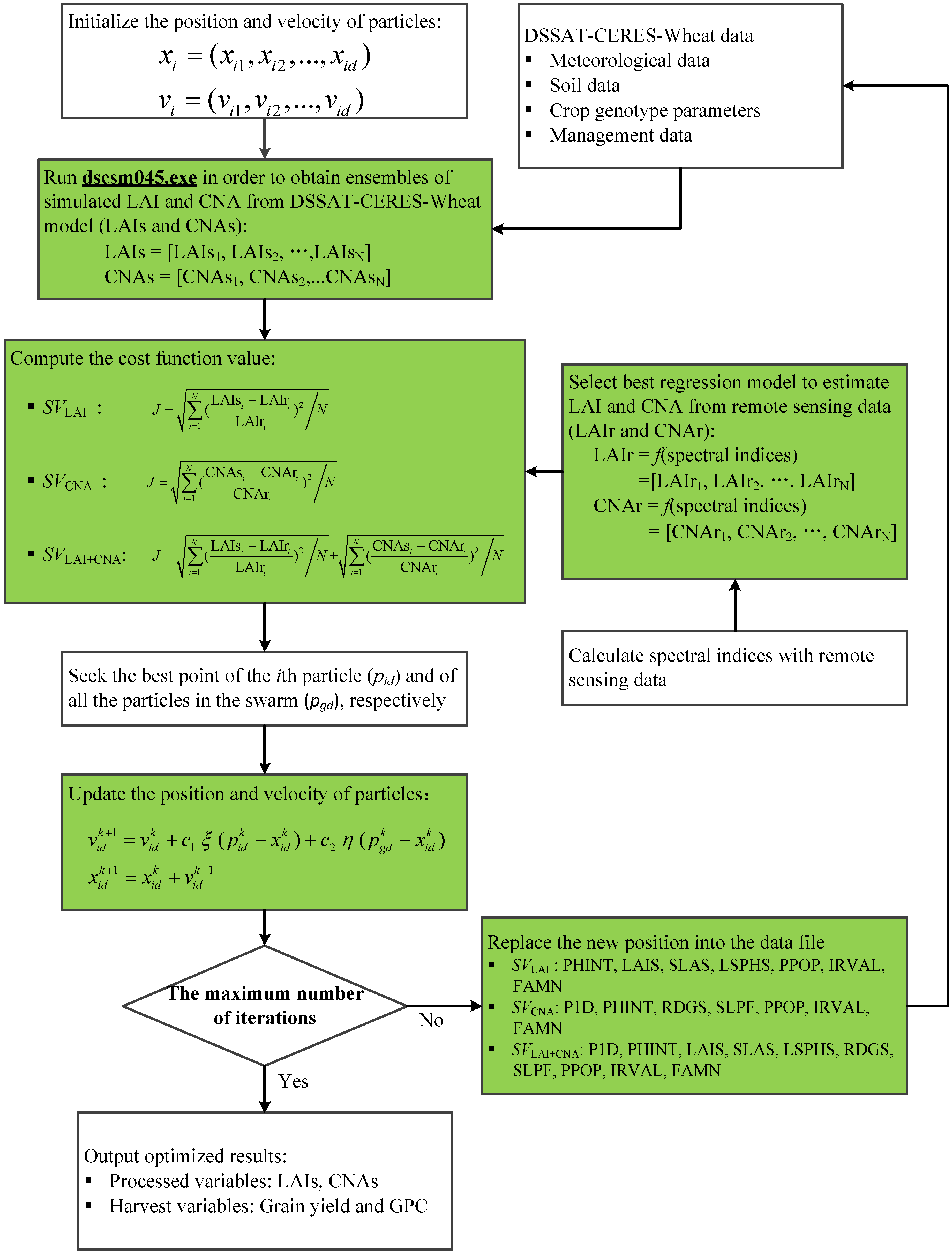
2.3.3. Data Assimilation Strategy

Kennedy and Eberhart [52] originally proposed particle swarm optimization (PSO) to simulate the graceful but unpredictable choreography of bird flocks [53]. In PSO, a particle is expressed a potential solution. Each particle, without quality or size in a d-dimensional search space, possesses its own position and velocity, and fitness value determined by a cost function. Every particle would modify its position and velocity associated with the optimal point in a current generation (pid) and that of all particles in a swarm (pgd). A flowchart for grain yield and GPC estimates made through the PSO assimilation of remote sensing data into the DSSAT-CERES model is illustrated in Figure 1.
In order to evaluate the assimilation performance of the two state variables, three assimilation schemes were conducted: only LAI as a state variable (SVLAI), only CNA as a state variable (SVCNA), and LAI and CNA used together as state variables (SVLAI + CNA). The detailed steps are as follows.
(1)
The initial value (position) and velocity of the particles were determined. For SVLAI, four crop genotype parameters (PHINT, LAIS, SLAS and LSPHS) sensitive to LAI and three management parameters (plant density, irrigation amount, and fertilization amount) were adjusted [54] (Table 4); For SVCNA, four crop genotype parameters (P1D, PHINT, RDGS and SLPF) sensitive to CNA and the same three management parameters were adjusted (Table 4). For SVLAI + CNA, all the above crop genotype and management parameters were considered. The velocity in each dimension was set to ~10% of the dynamic range of the variable [53]. It is important to point out that the parameters sensitive to CNA were set to default values (Table 4) in the SVLAI method, and vice versa (i.e., the parameters sensitive to LAI were set to default values (Table 4) in the SVCNA method).
(2)
The DSSAT executable file “dscsm045.exe” under the installation directory, integrated with the required data, was run in Matlab (version 2007, MathWorks, US), and the simulated LAI and CNA were output.
(3)
The relationships between the spectral indices and LAI or CNA were analyzed, and the best regression model was selected to estimate LAI and CNA, respectively.
(4)
The cost function was constructed according to the variables simulated by the DSSAT-CERES model and those retrieved by the spectral index. The fitness value from the cost function determined whether the optimization algorithm reached the optimum input parameters. When one state variable was used in an assimilation scheme (SVLAI or SVCNA), the cost function was based on only one variable (i.e., LAI or CNA) (Figure 1). When two state variables were used in an assimilation scheme (SVLAI + CNA), the cost function was based on both LAI and CNA.
(5)
The program searched for the pid and pgd at each iteration.
(6)
The positions and velocities of the particles were updated on the basis of pid and pgd. The c1 and c2 values were set as 2, and ξ and η were random values between 0 and 1 [53].
(7)
If the iteration (100 generations in this study) was not reached, the updated positions were replaced and the second step was conducted. If the iteration was reached, LAI, CNA, yield and GPC were output.

2.4. Statistical Analysis

The coefficient of determination (R2) and the root mean square error (RMSE) were used as metrics to quantify the amount of variation explained by the developed relationships, as well as the accuracy of those relationships. Generally, the performance of the model was estimated by comparing differences in the R2 and RMSE. A higher R2 and a lower RMSE indicated higher precision and accuracy of the inversion.
Figure 1. Flowchart of the particle swarm optimization (PSO) assimilation scheme for integrating remote sensing data with the Decision Support System for Agrotechnology Transfer–Crop Environment Resource Synthesis (DSSAT-CERES) model.
Remotesensing 07 12400 g001
Table 4. Initial values and ranges of calibration parameters or initial data of the DSSAT-CERES.
VariablesDefaultRanges
Initial data
Plant density (PPOP, m3)350300–400
Irrigation amount (IRVAL, mm)15090–240
Fertilization amount (FAMN, kg N∙ha1)2000–400
Sensitive to LAI
Phyllochron interval parameter (PHINT)10090–120
Area of standard first leaf (LA1S)2.01.5–3.0
Specific leaf area (SLAS)300200–400
Final leaf senescence starts (LSPHS)5.04.0–5.7
Sensitive to CNA
Photoperiod parameter (P1D)5030–70
Phyllochron interval parameter (PHINT)10090–120
Root depth growth rate (RDGS)3.02.5–3.5
Photosynthesis factor (SLPF)10.8–1.0
Note: The initial data values were determined with management data, and the genotype parameters were set based on default values in DSSAT-CERES model.

3. Results

3.1. LAI and CNA Estimation from Spectral Indices

Fifteen spectral indices were used to estimate winter wheat LAI and CNA from the field data from Experiments 1 and 2 (n = 100), and Experiment 3 (n = 32) was used to validate the models’ accuracy. Linear and nonlinear (logarithm, exponential, and power) functions were used to fit the models, and the best model had the highest R2 and lowest RMSE. Table 5 shows the relationship between LAI (or CNA) and the spectral indices.
The results show that all the spectral indices were significantly related to LAI (p-value < 0.001). In particular, the six indices (NDVI, MSR, OSAVI, WDRVI, GI and EVI) with R2 values greater than 0.8 best estimated the LAI of winter wheat, although large differences in their RMSE values (0.627, 0.598, 0.673, 0.651, 0.758 and 0.761, respectively) were revealed. The power relationship between MSR and LAI (R2 = 0.829, RMSE = 0.598) had the highest performance compared with the statistical relationships of the other indices, and this relationship was used to estimate the LAI of winter wheat in this study.
Similarly, the regressions between CNA and each spectral index (p-value < 0.001) were highly significant. In comparison, OSAVI, CIred-edge, MCARI/MTVI2, MTCI, NDRE and DCNII were more strongly related with CNA than the other indices, indicating they were very sensitive to changes in CNA (R2 = 0.701, 0.745, 0.762, 0.742, 0.794 and 0.733, respectively); the corresponding RMSE values used for validating the model accuracy were 39.97 kg N∙ha−1, 43.04 kg N∙ha−1, 42.73 kg N∙ha−1, 44.03 kg N∙ha−1, 37.75 kg N∙ha−1 and 52.43 kg N∙ha−1, respectively. NDRE had the highest R2 and the lowest RMSE, and the results showed that the predicted CNA was very consistent with the measured CNA (Table 5). Therefore, NDRE was selected to estimate the CNA of winter wheat in this study.
Table 5. Relationships of LAI and CNA with spectral indices of winter wheat (n = 100).
Spectral IndicesLAI ModelR2RMSECNA ModelR2RMSE (kg N∙ha1)
NDVIy = 0.1321e3.5882x0.800**0.627y = 3.1877e4.3454x0.699**41.80
MSRy = 0.89x0.97990.829**0.598y = 33.85x1.1320.659**44.52
OSAVIy = 0.2658e3.5008x0.826**0.673y = 317.72x2.22470.701**39.97
WDRVIy = 2.2473e1.5338x0.821**0.651y = 98.704e1.7295x0.622**47.62
CIred-edgey = 2.1067x0.82930.774**0.642y = 90.798x1.05440.745**43.04
GIy = 0.9191x1.84790.823**0.758y = 39.585x1.89030.513**53.36
VIopty = 4.7134x−12.9830.798**0.700y = 0.0239x6.99620.528**45.35
MCARI/MTVI2y = 0.0971x−1.0870.707**0.700y = 406.86e−23.41x0.762**42.73
MTCIy = 0.6336x1.03740.700**0.686y = 18.218x1.3830.742**44.03
sLAIDIy = 0.9837e1.5881x0.720**0.802y = 37.49e1.8599x0.588**37.13
EVIy = 6.7588x1.36720.812**0.761y = 362.97x1.61750.678**43.38
NDREy = 0.5172e3.5672x0.766**0.695y = 473.26x1.65250.794**37.75
NDCIy = 0.3319e4.5273x0.783**0.633y = 455.99x1.70350.478**47.12
DCNIIy = 0.5628e0.047x0.488**0.879y = 6.6829x−77.6680.733**52.43
TBWIy = 1.5433x0.51710.778**0.672y = 64.326x0.5890.601**44.14
Note: x represents spectral indices; y represents LAI (or CNA); probability levels are indicated by * and ** for p-values of 0.05 and 0.01, respectively.

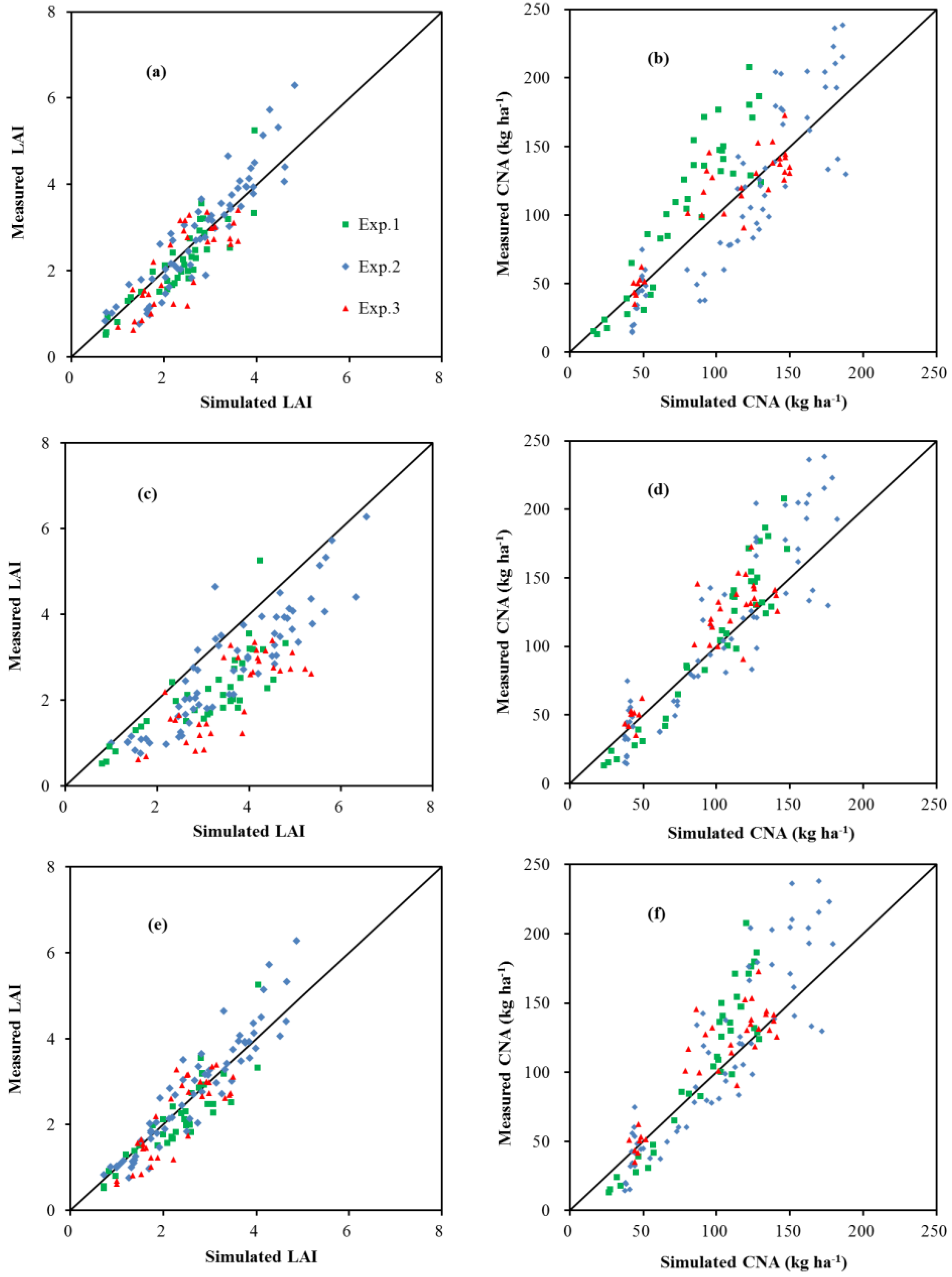
3.2. LAI and CNA Simulation Using Data Assimilation

According to the relationship between MSR and LAI and that between NDRE and CNA, LAI and CNA were used as state variables to calibrate the DSSAT-CERES model based on the PSO assimilation algorithm. The results shown in Figure 2 and Table 6 demonstrate a significant relationship between the simulated and measured LAI using the data assimilation methods. The SVLAI method used LAI as the state variable, and thus there was a strong linear relationship between the simulated and measured LAI (Figure 2a), with R2 values of 0.782, 0.857 and 0.637, and corresponding RMSE values of 0.452, 0.535 and 0.586 for Experiments 1, 2 and 3, respectively (Table 6). The SVCNA method used CNA as the state variable, and the simulated LAI was greater than the measured LAI (Figure 2c). The R2 and RMSE values between the simulated and measured LAI for Experiments 1, 2 and 3 were 0.619, 0.806 and 0.565, and 1.158, 1.001 and 1.579, respectively (Table 6). The SVLAI + CNA method used both LAI and CNA as state variables, and this method demonstrated a good simulation (Figure 2e), with R2 and RMSE values of 0.771, 0.873 and 0.670, and 0.472, 0.496 and 0.515 for Experiments 1, 2 and 3, respectively (Table 6). The relationships between the simulated and measured LAIs for the three experiments were analyzed together. The results show that there was a high variation in the SVCNA method’s estimates of LAI (R2 = 0.695; RMSE = 0.494), and the SVLAI + CNA method (R2 = 0.828; RMSE = 0.494) performed better than the single state variable method (R2 = 0.809; RMSE = 0.527 for the SVLAI method).
The simulated and measured CNA for the three assimilation methods were compared. The dispersion of the data between the simulated and measured CNA was larger with the SVLAI method. The results show that the SVLAI method tended to underestimate the CNA for Experiment 1 (R2 = 0.830; RMSE = 39.31 kg N∙ha−1), overestimate the CNA at low values for Experiment 2 (R2 = 0.793; RMSE = 32.14 kg N∙ha−1), and produce moderate results for Experiment 3 (R2 = 0.806; RMSE = 18.09 kg N∙ha−1) (Figure 2b and Table 6). The SVCNA method demonstrated a good consistency between the simulated and measured values of CNA (Figure 2d), with R2 and RMSE values of 0.902, 0.823 and 0.806, and 24.32 kg N∙ha−1, 31.71 kg N∙ha−1 and 21.45 kg N∙ha−1 for Experiments 1, 2 and 3, respectively (Table 6). For the SVLAI + CNA method, the R2 and RMSE values between the simulated and measured CNA for Experiments 1, 2 and 3 were 0.866, 0.816 and 0.788, and 31.20 kg N∙ha−1, 33.52 kg N∙ha−1 and 20.86 kg N∙ha−1, respectively (Table 6). The simulated CNA was in agreement with the measured CNA (Figure 2f). According to the three experiments, the best performance was produced by the SVCNA method (R2 = 0.833; RMSE = 27.58 kg N∙ha−1), followed by the SVLAI + CNA method (R2 = 0.808; RMSE = 30.26 kg N∙ha−1), and finally the SVLAI method (R2 = 0.715; RMSE = 31.65 kg N∙ha−1).
Figure 2. Relationships between simulated and measured values of (a) leaf area index (LAI) with LAI with a state variable (SVLAI), (b) canopy N accumulation (CNA) with SVLAI, (c) LAI with CNA with a state variable (SVCNA), (d) CNA with SVCNA, (e) LAI with SVLAI + CNA, and (f) CNA with SVLAI + CNA.
Remotesensing 07 12400 g002
Table 6. Regression equations between measured and simulated values of leaf area index (LAI) and canopy N accumulation (CNA) of winter wheat with three data assimilation methods across three experiments.
MethodExp.nRegression EquationR2RMSERegression EquationR2RMSE(kg N∙ha1)
SVLAI136y = 1.016x − 0.1840.7820.452y = 1.511x − 130.83039.31
264y = 1.19x − 0.4470.8570.535y = 1.231x − 29.950.79332.14
332y = 0.948x − 0.0880.6370.586y = 0.887x + 15.620.80618.09
All132y = 1.134x − 0.3960.8090.527y = 1.084x − 1.6730.71531.65
SVCNA136y = 0.662x + 0.110.6191.158y =1.406x − 31.330.90224.32
264y = 0.897x − 0.4360.8061.001y = 1.249x − 15.930.82331.71
332y = 0.682x − 0.2830.5651.579y = 1.038x + 9.230.80621.45
All132y = 0.809x − 0.3310.6951.207y = 1.247x − 14.540.83327.58
SVLAI + CNA136y = 0.975x − 0.1170.7710.472y = 1.586x − 39.040.86631.20
264y = 1.135x − 0.2430.8730.496y = 1.325x − 22.670.81633.52
332y = 1.009x − 0.1470.6700.515y = 1.005x + 10.260.78820.86
All132y = 1.107x − 0.2870.8280.494y = 1.304x − 18.220.80830.26

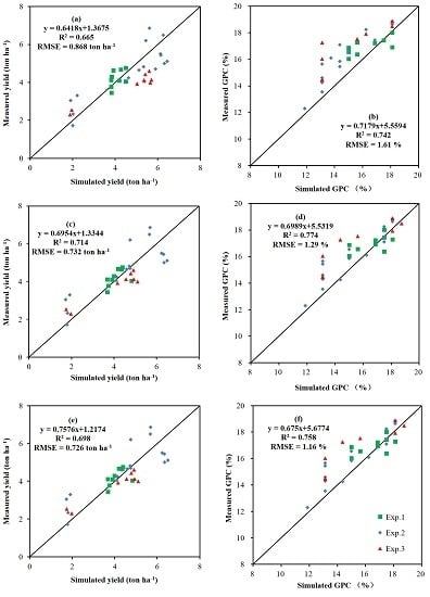
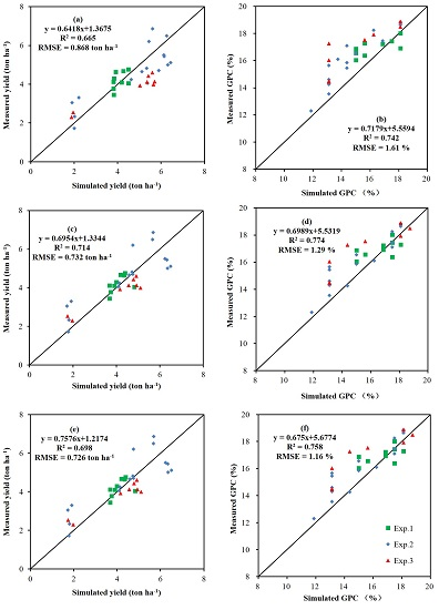
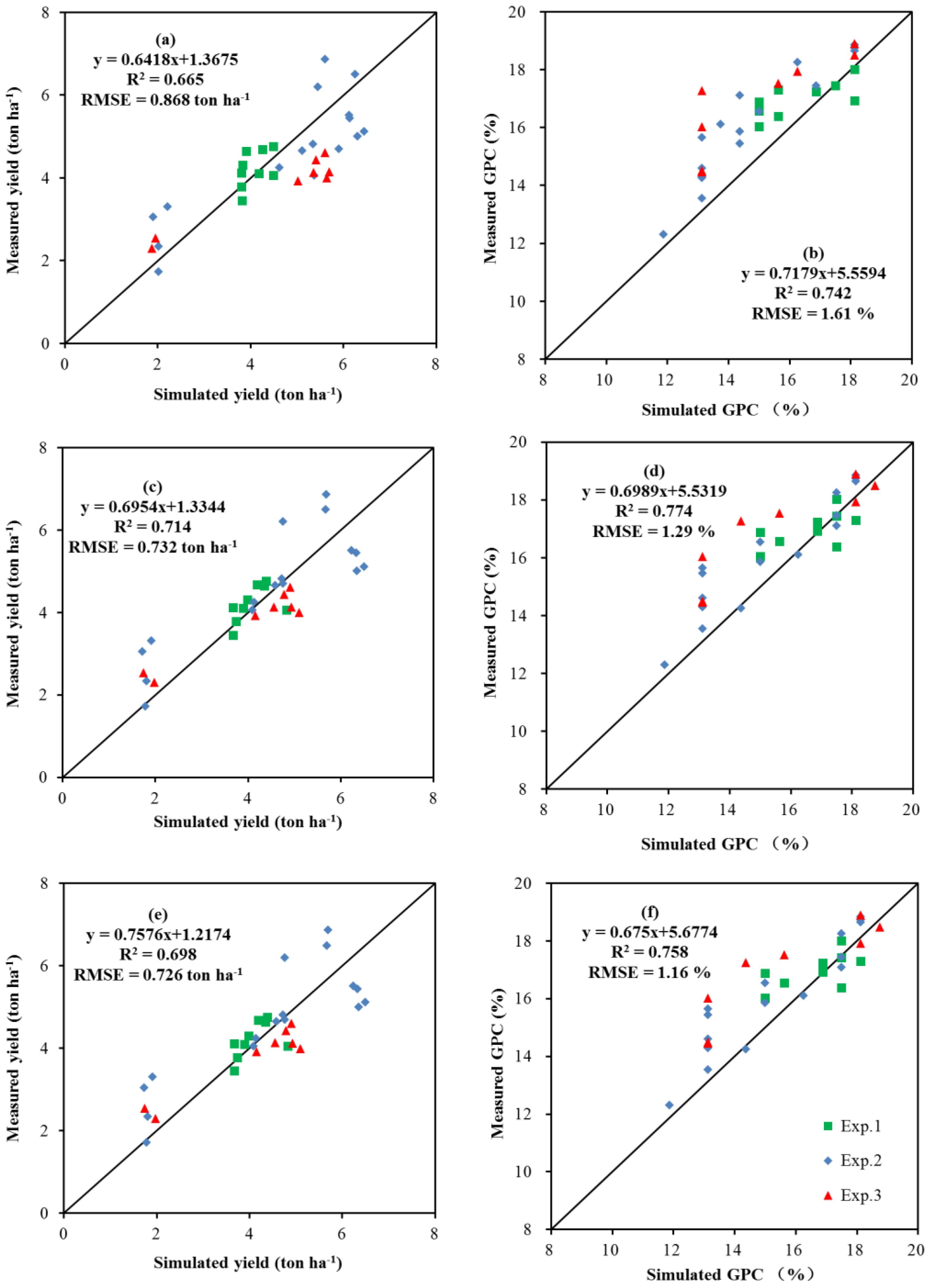
3.3. Grain Yield and GPC Estimation

The integration of remote sensing data and the DSSAT-CERES model was used to estimate the grain yield and GPC of winter wheat and the output estimate based on PSO. The relationships between the simulated and measured values of yield and GPC are shown in Figure 3. As Experiment 1 was just the sowing date and cultivar treatment, the range of the simulated yield was small. In contrast, Experiments 2 and 3 had a large range because of the different N and cultivar treatments. Scatter plots of the simulated and measured yields from the three data assimilation methods fit the one-to-one line well. Our results show that the SVCNA method (R2 = 0.714; RMSE = 0.732 ton∙ha−1) resulted in a better estimation of wheat yield than the SVLAI method (R2 = 0.665; RMSE = 0.868 ton∙ha−1 (Figure 3a,c). For the SVLAI + CNA method, the R2 and RMSE values between the simulated and measured yields were 0.698 and 0.726 ton∙ha−1, respectively (Figure 3e). With the smallest RMSE, the SVLAI + CNA method demonstrated the most consistency between simulated and measured values. In short, the data assimilation method with two state variables estimated grain yield with greater accuracy than that with only one state variable.
Similar results were obtained for the estimation of GPC by the three data assimilation methods, and a good linear relationship between simulated and measured GPC values was shown (Figure 3b,d,f). For the assimilation method with one state variable, the inversion of the SVCNA method (R2 = 0.774; RMSE = 1.29%) estimated GPC better than the SVLAI method (R2 = 0.742; RMSE = 1.61%). The R2 and RMSE values of the regression between the estimated and measured GPC values were 0.758 and 1.16% for the SVLAI + CNA method. The RMSE for the SVLAI + CNA method was lower than that for the data assimilation method with only one state variable. These results demonstrate the advantages of using two state variables for data assimilation.
Figure 3. Relationships between measured and simulated values of (a) yield with leaf area index as a state variable (SVLAI), (b) grain protein content (GPC) with SVLAI, (c) yield with canopy N accumulation as a state variable (SVCNA), (d) GPC with SVCNA, (e) yield with SVLAI + CNA, and (f) GPC with SVLAI + CNA.
Remotesensing 07 12400 g003

4. Discussion

Spectral indices from hyperspectral data were used to estimate the LAI and CNA of winter wheat, and these spectral indices had highly significantly relationships with LAI and CNA (Table 5). These spectral indices were constructed using red edge (670–780 nm) and shortwave infrared (NIR, 800–1100 nm) wavelengths and they contained useful information about the population size and nutritional status of wheat [41,55,56]. The regression between MSR and LAI (R2 = 0.829 and RMSE = 0.598) was better than those of the other indices and LAI. The MSR was expressed as a function of the simple ratio of NIR to red reflectance, and the simple ratio greatly reduced undesirable noise caused by simultaneous increases or decreases in red and NIR reflectance. The MSR also had the advantage of being less sensitive to canopy optical and geometrical properties [38]. Moreover, the MSR may have improved linearity and mitigated the saturation effect when LAI increased [57]. NDRE had the strongest relationship with CNA (R2 = 0.794 and RMSE = 37.75 kg N∙ha−1), and this index was measured with wavebands centered at 720 and 790 nm, which were more sensitive to estimating canopy N per unit area than canopy N concentration [48].
LAI and CNA were individually used as state variables for integrating remote sensing data into the DSSAT-CERES model with the PSO data assimilation method. The results show that each method (SVCNA and SVLAI) estimated LAI or CNA with great accuracy, in agreement with previous research [5], [7], [8], [16] and [17]. However, when only one assimilation variable was used, large errors existed between the simulated and measured values of the other variables; for example, the RMSE of LAI determined with the SVCNA method was 1.207, which was much larger than that determined with the SVLAI method (RMSE = 0.527). Likewise, the error between the simulated and measured values of CNA determined with the SVLAI method was larger than that determined with the SVCNA method. This problem was due to unwanted and inaccurate simulations because only one state variable (i.e. LAI or CNA) was accurately simulated.
In this study, the join usage of LAI and CNA as state variables for assimilating remote sensing information into the DSSAT-CERES model. The simulation with the combined variables was robust, with R2 and RMSE values of 0.828 and 0.494 for LAI and 0.808 and 30.26 kg N∙ha−1 for CNA. The accuracy of the state variable simulations made using two assimilation variables was fairly consistent or even better than those using one variable (LAI or CNA). The primary reason for this is that LAI is a key variable for crop growth monitoring and yield prediction [58], and CNA is an important indicator of the N status of wheat and significantly affects photosynthetic production and grain yield and quality [59]. Various crop state variables are independent of each other, though they interact with each other [18,60]. Therefore, the SVLAI + CNA method obtained a greater robustness of the DSSAT-CERES model than the single variable methods. However, this study only investigated LAI (a crop population indicator) and CNA (a nutritional status indicator), and the combination of these two state variables may not have been optimal, as the matching of the pattern of interaction between these state variables in a natural system may not yet be fit by the interaction pattern between them within the simulated system. In addition, the cost function was constructed by simple addition (Figure 1), and it did not consider the different deviations between simulated and measured values. Therefore, future studies should pay attention to two points: (1) how to select two optimal state variables that can achieve robust simulations for most model outputs; and (2) how to determine the cost function when two state variables are considered.
According to the results of the grain yield and GPC estimations, the inverted SVCNA method estimated grain yield and GPC better than the SVLAI method (Figure 3a–d). This is because CNA is determined by actual plant N concentration and the corresponding canopy biomass of each plant organ [32,35], thus, nutrient status and plant biomass are simultaneously considered in crop growth. The joint use of LAI and CNA as state variables also obtained good estimations of grain yield and GPC, and the RMSE values between the simulated and measured grain yield and GPC were the lowest. Grain yield is derived from the partition of fixed carbon, which is directly related with LAI [33]. Similarly, grain N accumulation is derived from the re-translocation of CNA, and GPC is simply calculated as the N concentration in grain multiplied by a factor [32,36]. The assimilation of two state variables derived from a remote sensor mutually promoted consistent results between the simulated and measured values of grain yield and GPC.
Integrating remote sensing data with the DSSAT-CERES model for grain yield and GPC estimation could feasibly be conducted with different sowing dates, cultivars, and N management strategies across different years in this study. Further efforts are required to couple satellite data with the DSSAT-CERES model for estimating grain yield and GPC at a regional scale.

5. Conclusions

The joint integration of remotely sensed LAI and CNA as state variables into the DSSAT-CERES model using the PSO algorithm was tested in this study. The results suggested that LAI and CNA were accurately estimated with spectral indices, and MSR and NDRE were the best indices for estimating LAI and CNA, respectively. The method of jointly integrating LAI and CNA as state variables was more robust than single variable integration. A good accuracy of winter wheat grain yield and GPC estimations was demonstrated using this kind of data assimilation method. The results demonstrated integrating remote sensing with the DSSAT-CERES model is a potential approach for estimating grain yield and especially GPC.

Acknowledgments

This study was supported by the National Natural Science Foundation of China (Grant No. 41471285, 41171281), Science and Technology Innovation Capability Construction of Beijing Academy of Agriculture and Forestry Sciences (Grant No.KJCX20150409), and the Beijing Natural Science Foundation (Grant No. 4141001, 6132015). We are grateful to the China Meteorological Data Sharing Service System for collecting the environmental data and to Weiguo Li, Qian Wang, Hong Chang and Ling Kong for collecting the soil data. Finally, we very much appreciate the editors and anonymous reviewers who provided useful comments.

Author Contributions

Zhenhai Li analyzed data and wrote the manuscript. Jihua Wang, Chunjiang Zhao, Xingang Xu, Xiuliang Jin and Guijun Yang gave comments, suggestions to the manuscript, and checked the writing. Haikuan Feng, Zhenhai Li and Xiuliang Jin provided data and data acquisition capacity.

Conflicts of Interest

The authors declare no conflict of interest.

References

  1. Yu, Z.W. Crop Cultivation; China Agriculture Press: Beijing, China, 2003. [Google Scholar]
  2. Li, C.; Wang, J.; Wang, Q.; Wang, D.; Song, X.; Wang, Y.; Huang, W. Estimating wheat grain protein content using multi-temporal remote sensing data based on partial least squares regression. J. Integr. Agr. 2012, 11, 1445–1452. [Google Scholar] [CrossRef]
  3. Reynolds, M.; Foulkes, J.; Furbank, R.; Griffiths, S.; King, J.; Murchie, E.; Parry, M.; Slafer, G. Achieving yield gains in wheat. Plant Cell Environ. 2012, 35, 1799–1823. [Google Scholar] [CrossRef] [PubMed]
  4. Liu, L.Y.; Wang, J.J.; Bao, Y.S.; Huang, W.J.; Ma, Z.H.; Zhao, C.J. Predicting winter wheat condition, grain yield and protein content using multi-temporal EnviSat-ASAR and Landsat TM satellite images. Int. J. Remote Sens. 2006, 27, 737–753. [Google Scholar] [CrossRef]
  5. Thorp, K.R.; White, J.W.; Porter, C.H.; Hoogenboom, G.; Nearing, G.S.; French, A.N. Methodology to evaluate the performance of simulation models for alternative compiler and operating system configurations. Comput. Electron. Agr. 2012, 81, 62–71. [Google Scholar] [CrossRef]
  6. Zhang, Q.; Xiao, X.; Braswell, B.; Linder, E.; Baret, F.; Moore, B., III. Estimating light absorption by chlorophyll, leaf and canopy in a deciduous broadleaf forest using MODIS data and a radiative transfer model. Remote Sens. Environ. 2005, 99, 357–371. [Google Scholar] [CrossRef]
  7. Fang, H.; Liang, S.; Hoogenboom, G.; Teasdale, J.; Cavigelli, M. Corn-yield estimation through assimilation of remotely sensed data into the CSM-CERES-Maize model. Int. J. Remote Sens. 2008, 29, 3011–3032. [Google Scholar] [CrossRef]
  8. Guerif, M.; Duke, C.L. Adjustment procedures of a crop model to the site specific characteristics of soil and crop using remote sensing data assimilation. Agr. Ecosyst. Environ. 2000, 81, 57–69. [Google Scholar] [CrossRef]
  9. Maas, S.J. Use of remotely-sensed information in agricultural crop growth models. Ecol. Model. 1988, 41, 247–268. [Google Scholar] [CrossRef]
  10. Maas, S.J. Using satellite data to improve model estimates of crop yield. Agron. J. 1988, 80, 655–662. [Google Scholar] [CrossRef]
  11. Guerif, M.; Duke, C. Calibration of the SUCROS emergence and early growth module for sugar beet using optical remote sensing data assimilation. Eur. J. Agron. 1998, 9, 127–136. [Google Scholar] [CrossRef]
  12. Jongschaap, R.E. Run-time calibration of simulation models by integrating remote sensing estimates of leaf area index and canopy nitrogen. Eur. J. Agron. 2006, 24, 316–324. [Google Scholar] [CrossRef]
  13. De Wit, A.; Van Diepen, C.A. Crop model data assimilation with the Ensemble Kalman filter for improving regional crop yield forecasts. Agr. Forest Meteorol. 2007, 146, 38–56. [Google Scholar] [CrossRef]
  14. Fang, H.; Liang, S.; Hoogenboom, G. Integration of MODIS LAI and vegetation index products with the CSM-CERES-Maize model for corn yield estimation. Int. J. Remote Sens. 2011, 32, 1039–1065. [Google Scholar] [CrossRef]
  15. Morel, J.; Begue, A.; Todoroff, P.; Martine, J.; Lebourgeois, V.; Petit, M. Coupling a sugarcane crop model with the remotely sensed time series of fIPAR to optimise the yield estimation. Eur. J. Agron. 2014, 61, 60–68. [Google Scholar] [CrossRef]
  16. Li, Y.; Zhou, Q.; Zhou, J.; Zhang, G.; Chen, C.; Wang, J. Assimilating remote sensing information into a coupled hydrology-crop growth model to estimate regional maize yield in arid regions. Ecol. Model. 2014, 291, 15–27. [Google Scholar] [CrossRef]
  17. Dong, Y.; Zhao, C.; Yang, G.; Chen, L.; Wang, J.; Feng, H. Integrating a very fast simulated annealing optimization algorithm for crop leaf area index variational assimilation. Math. Comput. Model. 2013, 58, 877–885. [Google Scholar] [CrossRef]
  18. Wang, H.; Zhu, Y.; Li, W.; Cao, W.; Tian, Y. Integrating remotely sensed leaf area index and leaf nitrogen accumulation with RiceGrow model based on particle swarm optimization algorithm for rice grain yield assessment. J. Appl. Remote Sens. 2014, 8, 083674. [Google Scholar] [CrossRef]
  19. Thorp, K.R.; Wang, G.; West, A.L.; Moran, M.S.; Bronson, K.F.; White, J.W.; Mon, J. Estimating crop biophysical properties from remote sensing data by inverting linked radiative transfer and ecophysiological models. Remote Sens. Environ. 2012, 124, 224–233. [Google Scholar] [CrossRef]
  20. Ma, H.Y. Winter Wheat Yield Estimation Based on Assimilating Leaf Area Index and Evapotranspiration into SWAP Crop Model. Ph.D. Thesis, China Agricultural University, Beijing, China, 2013. [Google Scholar]
  21. China Meteorological Data Sharing Service System. Available online: http://cdc.cma.gov.cn (accessed on 12 September 2015).
  22. Allen, R.G.; Pereira, L.S.; Raes, D.; Smith, M. Crop Evapotranspiration: Guidelines for Computing Crop Water Requirements, FAO Irrigation and Drainage Paper No. 56; FAO: Rome, Italy, 1998; Volume 300, p. d05109. [Google Scholar]
  23. Wang, J.H.; Zhao, C.J.; Huang, W.J. Basis and Application of Agriculture Quantitative Remote Sensing; Science Press: Beijing, China, 2008. [Google Scholar]
  24. Zadoks, J.C.; Chang, T.T.; Konzak, C.F. A decimal code for the growth stages of cereals. Weed Res. 1974, 14, 415–421. [Google Scholar] [CrossRef]
  25. Breda, N.J. Ground-based measurements of leaf area index: a review of methods, instruments and current controversies. J. Exp. Bot. 2003, 54, 2403–2417. [Google Scholar] [CrossRef] [PubMed]
  26. Schepers, J.S.; Francis, D.D.; Thompson, M.T. Simultaneous determination of total C, total N, and 15N on soil and plant material. Commun. Soil Sci. Plan. Anal. 1989, 20, 949–959. [Google Scholar] [CrossRef]
  27. Palosuo, T.; Kersebaum, K.C.; Angulo, C.; Hlavinka, P.; Moriondo, M.; Olesen, J.E.; Patil, R.H.; Ruget, F.; Rumbaur, C.; Takáč, J. Simulation of winter wheat yield and its variability in different climates of Europe: A comparison of eight crop growth models. Eur. J. Agron. 2011, 35, 103–114. [Google Scholar] [CrossRef]
  28. Thorp, K.R.; DeJonge, K.C.; Kaleita, A.L.; Batchelor, W.D.; Paz, J.O. Methodology for the use of DSSAT models for precision agriculture decision support. Comput. Electron. Agrc. 2008, 64, 276–285. [Google Scholar] [CrossRef]
  29. Jones, J.W.; Hoogenboom, G.; Porter, C.H.; Boote, K.J.; Batchelor, W.D.; Hunt, L.A.; Wilkens, P.W.; Singh, U.; Gijsman, A.J.; Ritchie, J.T. The DSSAT cropping system model. Eur. J. Agron. 2003, 18, 235–265. [Google Scholar] [CrossRef]
  30. Ritchie, J.T. Wheat phasic development. In Modeling Plant and Soil Systems; Hanks, J., Ritchie, J.T., Eds.; American Society of Agronomy, Crop Science Society of America, Soil Science Society of America: Madison, WI, USA, 1991; pp. 31–54. [Google Scholar]
  31. Nearing, G.S.; Crow, W.T.; Thorp, K.R.; Moran, M.S.; Reichle, R.H.; Gupta, H.V. Assimilating remote sensing observations of leaf area index and soil moisture for wheat yield estimates: An observing system simulation experiment. Water Resour. Res. 2012, 48, W05525. [Google Scholar] [CrossRef]
  32. Ritchie, J.T.; Godwin, D. CERES Wheat 2.0. Available online: http://nowlin.css.msu.edu/indexritchie.html (accessed on 12 September 2015).
  33. Thorp, K.R.; Hunsaker, D.J.; French, A.N.; White, J.W.; Clarke, T.R.; Pinter, P.J., Jr. Evaluation of the CSM-CROPSIM-CERES-Wheat model as a tool for crop water management. Trans. ASABE 2010, 53, 87–102. [Google Scholar] [CrossRef]
  34. DeJonge, K.C.; Ascough, J.C.; Ahmadi, M.; Andales, A.A.; Arabi, M. Global sensitivity and uncertainty analysis of a dynamic agroecosystem model under different irrigation treatments. Ecol. Model. 2012, 231, 113–125. [Google Scholar] [CrossRef]
  35. Liu, H.L.; Yang, J.Y.; Drury, C.A.; Reynolds, W.D.; Tan, C.S.; Bai, Y.L.; He, P.; Jin, J.; Hoogenboom, G. Using the DSSAT-CERES-Maize model to simulate crop yield and nitrogen cycling in fields under long-term continuous maize production. Nutr. Cycl. Agroecosys. 2011, 89, 313–328. [Google Scholar] [CrossRef]
  36. Asseng, S.; Bar-Tal, A.; Bowden, J.W.; Keating, B.A.; Van Herwaarden, A.; Palta, J.A.; Huth, N.I.; Probert, M.E. Simulation of grain protein content with APSIM-Nwheat. Eur. J. Agron. 2002, 16, 25–42. [Google Scholar] [CrossRef]
  37. Pearson, R.L.; Miller, L.D. Remote mapping of standing crop biomass for estimation of the productivity of the short grass prairie. In Proceedings of 8th International Symposium on Remote Sensing of the Environment, Michigan, USA, 2–6 October 1972; pp. 1355–1379.
  38. Chen, J.M. Evaluation of vegetation indices and a modified simple ratio for boreal applications. Can. J. Remote Sens. 1996, 22, 229–242. [Google Scholar] [CrossRef]
  39. Rondeaux, G.; Steven, M.; Baret, F. Optimization of soil-adjusted vegetation indices. Remote Sens. Environ. 1996, 55, 95–107. [Google Scholar] [CrossRef]
  40. Gitelson, A.A. Wide dynamic range vegetation index for remote quantification of biophysical characteristics of vegetation. J. Plant Physiol. 2004, 161, 165–173. [Google Scholar] [CrossRef] [PubMed]
  41. Gitelson, A.A.; Vina, A.; Ciganda, V.; Rundquist, D.C.; Arkebauer, T.J. Remote estimation of canopy chlorophyll content in crops. Geophys. Res. Lett. 2005, 32, L08403. [Google Scholar] [CrossRef]
  42. Zarco-Tejada, P.J.; Berjón, A.; López-Lozano, R.; Miller, J.R.; Martín, P.; Cachorro, V.; González, M.R.; De Frutos, A. Assessing vineyard condition with hyperspectral indices: Leaf and canopy reflectance simulation in a row-structured discontinuous canopy. Remote Sens. Environ. 2005, 99, 271–287. [Google Scholar] [CrossRef]
  43. Reyniers, M.; Walvoort, D.J.; De Baardemaaker, J. A linear model to predict with a multi-spectral radiometer the amount of nitrogen in winter wheat. Int. J. Remote Sens. 2006, 27, 4159–4179. [Google Scholar] [CrossRef]
  44. Eitel, J.U.H.; Long, D.S.; Gessler, P.E.; Smith, A.M.S. Using in-situ measurements to evaluate the new RapidEye™ satellite series for prediction of wheat nitrogen status. Int. J. Remote Sens. 2007, 28, 4183–4190. [Google Scholar] [CrossRef]
  45. Dash, J.; Curran, P.J. Evaluation of the MERIS terrestrial chlorophyll index (MTCI). Adv. Space Res. 2007, 39, 100–104. [Google Scholar] [CrossRef]
  46. Delalieux, S.; Somers, B.; Hereijgers, S.; Verstraeten, W.W.; Keulemans, W.; Coppin, P. A near-infrared narrow-waveband ratio to determine Leaf Area Index in orchards. Remote Sens. Environ. 2008, 112, 3762–3772. [Google Scholar] [CrossRef]
  47. Jiang, Z.; Huete, A.R.; Didan, K.; Miura, T. Development of a two-band enhanced vegetation index without a blue band. Remote Sens. Environ. 2008, 112, 3833–3845. [Google Scholar] [CrossRef]
  48. Fitzgerald, G.; Rodriguez, D.; O Leary, G. Measuring and predicting canopy nitrogen nutrition in wheat using a spectral index—The canopy chlorophyll content index (CCCI). Field Crop. Res. 2010, 116, 318–324. [Google Scholar] [CrossRef]
  49. Mishra, S.; Mishra, D.R. Normalized difference chlorophyll index: A novel model for remote estimation of chlorophyll-a concentration in turbid productive waters. Remote Sens. Environ. 2012, 117, 394–406. [Google Scholar] [CrossRef]
  50. Jin, X.; Xu, X.; Song, X.; Li, Z.; Wang, J.; Guo, W. Estimation of leaf water content in winter wheat using grey relational analysis-partial least squares modeling with hyperspectral data. Agron. J. 2013, 105, 1385–1392. [Google Scholar] [CrossRef]
  51. Jin, X.; Li, Z.; Feng, H.; Xu, X.; Yang, G. Newly combined spectral indices to improve estimation of total leaf chlorophyll content in cotton. IEEE J. Sel. Topics Appl. Earth Obs. Remote Sens. 2014, 7, 4589–4600. [Google Scholar] [CrossRef]
  52. Eberhart, R.C.; Kennedy, J. A new optimizer using particle swarm theory. In Proceedings of the Sixth International Symposium on Micro Machine and Human Science, Nagoya, Japan, 19–21 September 2006; pp. 39–43.
  53. Eberhart, R.C.; Shi, Y.H. Particle swarm optimization: Developments, applications and resources. In Proceedings of the 2001 IEEE Congress on Evolutionary Computation, Seoul, Korea, 27–30 May 2001.
  54. Li, Z.H.; Jin, X.L.; Liu, H.L.; Xu, X.G.; Wang, J.H.; Li, C.J. Global sensitivity analysis of wheat grain yield and quality and the related process variables from the DSSAT-CERES model based on the extended Fourier Amplitude Sensitivity Test method. Field Crop. Res. 2015. under review. [Google Scholar]
  55. Vincini, M.; Frazzi, E.; D’Alessio, P. Angular dependence of maize and sugar beet VIs from directional Compact High Resolution Imaging Spectrometer/Project for On-Board Autonomy (CHRIS/Proba) data. In Proceedings of 4th ESA CHRIS PROBA Workshop, Frascati, Italy, 19–21 September 2006.
  56. Sims, D.A.; Gamon, J.A. Relationships between leaf pigment content and spectral reflectance across a wide range of species, leaf structures and developmental stages. Remote Sens. Environ. 2002, 81, 337–354. [Google Scholar] [CrossRef]
  57. Haboudane, D.; Miller, J.R.; Pattey, E.; Zarco-Tejada, P.J.; Strachan, I.B. Hyperspectral vegetation indices and novel algorithms for predicting green LAI of crop canopies: Modeling and validation in the context of precision agriculture. Remote Sens. Environ. 2004, 90, 337–352. [Google Scholar] [CrossRef]
  58. Jin, X.; Diao, W.; Xiao, C.; Wang, F.; Chen, B.; Wang, K.; Li, S. Estimation of Wheat Agronomic Parameters using New Spectral Indices. PLoS ONE 2013, 8, e72736. [Google Scholar] [CrossRef] [PubMed]
  59. Feng, W.; Yao, X.; Zhu, Y.; Tian, Y.C.; Cao, W.X. Monitoring leaf nitrogen status with hyperspectral reflectance in wheat. Eur. J. Agron. 2008, 28, 394–404. [Google Scholar] [CrossRef]
  60. Wang, J.; Li, X.; Lu, L.; Fang, F. Parameter sensitivity analysis of crop growth models based on the extended Fourier Amplitude Sensitivity Test method. Environ. Modell. Softw. 2013, 48, 171–182. [Google Scholar] [CrossRef]

