Next Article in Journal
Removal of Thin Clouds in Landsat-8 OLI Data with Independent Component Analysis
Next Article in Special Issue
Assimilation of Two Variables Derived from Hyperspectral Data into the DSSAT-CERES Model for Grain Yield and Quality Estimation
Previous Article in Journal
Use of A Portable Camera for Proximal Soil Sensing with Hyperspectral Image Data
 
 
Correction published on 19 December 2015, see Remote Sens. 2015, 7(12), 17291-17296.
Article

Fusion of Plant Height and Vegetation Indices for the Estimation of Barley Biomass

Institute of Geography, GIS & RS, University of Cologne, D-50923 Cologne, Germany
*
Author to whom correspondence should be addressed.
Remote Sens. 2015, 7(9), 11449-11480; https://doi.org/10.3390/rs70911449
Submission received: 22 June 2015 / Revised: 23 August 2015 / Accepted: 2 September 2015 / Published: 9 September 2015
(This article belongs to the Special Issue Remote Sensing in Precision Agriculture)

Abstract

:
Plant biomass is an important parameter for crop management and yield estimation. However, since biomass cannot be determined non-destructively, other plant parameters are used for estimations. In this study, plant height and hyperspectral data were used for barley biomass estimations with bivariate and multivariate models. During three consecutive growing seasons a terrestrial laser scanner was used to establish crop surface models for a pixel-wise calculation of plant height and manual measurements of plant height confirmed the results (R2 up to 0.98). Hyperspectral reflectance measurements were conducted with a field spectrometer and used for calculating six vegetation indices (VIs), which have been found to be related to biomass and LAI: GnyLi, NDVI, NRI, RDVI, REIP, and RGBVI. Furthermore, biomass samples were destructively taken on almost the same dates. Linear and exponential biomass regression models (BRMs) were established for evaluating plant height and VIs as estimators of fresh and dry biomass. Each BRM was established for the whole observed period and pre-anthesis, which is important for management decisions. Bivariate BRMs supported plant height as a strong estimator (R2 up to 0.85), whereas BRMs based on individual VIs showed varying performances (R2: 0.07–0.87). Fused approaches, where plant height and one VI were used for establishing multivariate BRMs, yielded improvements in some cases (R2 up to 0.89). Overall, this study reveals the potential of remotely-sensed plant parameters for estimations of barley biomass. Moreover, it is a first step towards the fusion of 3D spatial and spectral measurements for improving non-destructive biomass estimations.

Graphical Abstract

1. Introduction

Over the past several decades remote sensing has increased in importance for precision agriculture [1,2,3]. Since the world population is expected to increase by more than one third until 2050 a main goal is shrinking the gap between potential and current yield [4,5]. Field management strategies in precision agriculture that aim to maximize yield must involve a reasonable use of natural resources and have to take spatial and temporal variabilities into account [6], as agricultural production is influenced by the physical landscape, climatic variables, and agricultural management practices [2]. Studies reveal that grain yield is correlated with total biomass [7,8]. A quantitative measure is the harvest index, which expresses yield vs. total biomass [9]. Moreover, adequate crop condition in early growing stages could buffer the yield against environmental stresses, such as droughts, during later stages [10]. In-season, the nitrogen nutrition index, the ratio between actual and critical nitrogen (N) content, is widely used as a measure of the plant status [11]. The critical value is defined by a crop-specific N dilution curve, showing the relation between N concentration and biomass. Hence, an exact in-season acquisition of biomass is important in precision agriculture.
Since plant biomass cannot be determined non-destructively, other plant parameters are used as estimators. Therefore, remote sensing measurements enable an objective and accurate acquisition in a high temporal frequency [2]. A review of remote sensing methods for assessing biomass is given by Ahamed et al. [12]. At the field level, ground-based methods are commonly used to achieve sufficiently high resolutions and over the last several decades, several studies investigated the relationship between spectral reflectance measurements and crop characteristics. For extracting information, various vegetation indices (VIs) were developed from the reflectance in determined wavelengths. Two band VIs like the normalized difference vegetation index (NDVI) were traditionally used with multispectral broad band systems to estimate biomass or biomass related parameters, like LAI. Such VIs have been adapted to narrow band hyperspectral data and other band combinations [13,14,15,16]. Additionally, other VIs with more than two bands, such as the GnyLi, have been developed for the same purpose [17].
Moreover, active sensors based on light detection and ranging (LiDAR) have been increasingly used in vegetation studies since the 1980s [18]. Indeed, a main benefit of LiDAR is the very high resolution, which enables the acquisition of complex canopies [19]. In agricultural applications, for example, ground-based LiDAR methods, also known as terrestrial laser scanning (TLS), reveal potential for assessing plant height [20], leaf area index [21], crop density [22,23,24], or post-harvest growth [25]. Furthermore, the potential for estimating biomass with TLS is supported through studies on small grain cereals [26,27,28], sagebrush [29], and paddy rice [30,31]. The 3D architecture of single plants was modeled under laboratory conditions [32,33], however the transferability of those laboratory results to field conditions has not yet been shown.
Generally, the accuracy of estimations is a major issue, with the accuracy being limited when calculations are based on one estimator. Whilst biomass estimations based on VIs are affected by saturation effects [13,34,35], plant height may reach limitations when differences in plant height are low. Consequently, the fusion of multiple parameters should be examined to enhance estimations. So far, studies on the fusion of spectral and non-spectral information have been applied for characterization of forest ecosystems [36] and modeling of corn yield [37]. As both studies applied airborne methods, the spatial resolution was low. A ground-based multi-sensor approach for predicting biomass of grassland based on measurements of plant height, leaf area index (LAI), and spectral reflectance showed that combining multiple sensors can improve the estimation [34]. However, in that study, spectral data were not well-suited. Recently, the potential of the combined use of spectral and non-spectral ground-based measurements for estimating biomass was demonstrated for rice, maize, cotton, and alfalfa [15].
The overall aim of this study was to compare the potential of plant height (PH), VIs, and a fusion of PH and VIs for estimations of above ground fresh and dry barley biomass. More specifically, this study compares the potential of 3D spatial and spectral information for different time frames during the growing season and investigates if a fusion of both can improve the estimation. Therefore, a spring barley experiment was monitored during three growing seasons in various campaigns with a TLS system and a field spectrometer. PH was derived from the TLS data and VIs from the hyperspectral data. Four major working tasks were carried out: (i) conduct extensive multi-annual field measurements during the growing seasons, (ii) derive bivariate biomass regression models (BRMs) from 3D spatial and spectral measurements for biomass estimations, (iii) fuse the 3D spatial and spectral data in multivariate BRMs to estimate biomass based on this extensive data set, and (iv) evaluate the robustness of the BRMs with a cross-validation.

2. Methods

2.1. Field Measurements

In three growing seasons (2012, 2013 and 2014), field experiments were carried out at the Campus Klein-Altendorf (50°37′51″N, E 6°59′32″) belonging to the Faculty of Agriculture at the University of Bonn, Germany. Due to crop rotation, the locations of the fields were slightly different between the years. However, soil and climatic conditions were similar with the surface of the soil being flat with a clayey silt luvisol and well-suited for crop cultivation [38]. According to the campus’ own weather records, the long-term average yearly precipitation was about 600 mm with a daily average temperature of 9.3 °C [39].
Each year, the field consisted of 36 small scale plots (3 × 7 m) where different cultivars of barley were cultivated with two levels of N fertilization. For half of the plots, a farmer’s common rate of 80 kg/ha∙N fertilizer was applied, for the other half a reduced rate of 40 kg/ha. In 2012 and 2013 each fertilization scheme was carried out once for 18 cultivars of spring barley (Barke, Wiebke, Beatrix, Eunova, Djamila, Streif, Ursa, Victoriana, Sissy, Perun, Apex, Isaria, Trumpf, Pflugs Intensiv, Heils Franken, Ackermanns Bavaria, Mauritia and Sebastian). In 2014, the set-up for the experiment was changed in that each fertilization scheme was repeated three times for six selected cultivars (Barke, Beatrix, Eunova, Trumpf, Mauritia and Sebastian). The experiments were carried out within the interdisciplinary research network CROP.SENSe.net (www.cropsense.uni-bonn.de). The research focus of this project was non-destructive sensor-based methods for detecting crop status such as nutrients, stress, and quality.
In this study, 3D spatial measurements from a TLS system, spectral measurements from a field spectrometer, and manual reference measurements were used. Due to the weather conditions the time of seeding changed and therefore so did the start of the growing season. The seeding dates were 21 March 2012, 9 April 2013, and 13 March 2014. In Table 1, all dates of TLS and spectrometer campaigns are listed as day after seeding (DAS) and a universal scale, known as the BBCH scale, was used to describe phenological stages and steps in the plant development, encoded in a decimal code [40,41]. The acronym BBCH is derived from the funding organizations: Biologische Bundesanstalt (German Federal Biological Research Centre for Agriculture and Forestry), Bundessortenamt (German Federal Office of Plant Varieties), and Chemical industry. The first number of the two-digit code represents the principal growth stage (Table 2) and the second subdivides further in short developmental steps. Through determining the BBCH codes during the growing seasons, the annual comparability was ensured. For each plot, the BBCH developmental step was determined as a mean of three plants. In Table 1, BBCH codes are given for the dates where plant parameters were manually measured. The codes are averaged per campaign, as the values were almost similar for all cultivars. Although the plant development varied among the years it can be seen that the BBCH codes indicate a comparable development.
As reference measurements, the heights of ten plants were measured for each plot and averaged in the post-processing. Moreover, in a defined sampling area of each plot, the above ground biomass of a 0.2 × 0.2 m area was destructively taken each time. The sampling area was neglected for the remote sensing measurements. In the laboratory, plants were cleaned and fresh weights were measured. After drying the samples for 120 h at 70 °C, dry biomass was weighted and extrapolated across the plot (g/m²).

2.1.1. Terrestrial Laser Scanning

The TLS configuration and setup was almost equal in all years. Thus for each campaign, the time-of-flight scanner Riegl LMS-Z420i was used (Figure 1A) [42]. The sensor operates with a near-infrared laser beam, has a beam divergence of 0.25 mrad, and a measurement rate of up to 11,000 points/sec. In addition its field of view is up to 80° in the vertical and 360° in the horizontal direction and this study used resolutions between 0.034° and 0.046°. The digital camera Nikon D200 was mounted on the laser scanner and the TLS point clouds were colorized from the images captured. Furthermore the sensor should be as high as possible above ground, resulting in a steep angle between scanner and investigated area enabling the best possible coverage of the crop surface and a homogenous penetration of the vegetation. Accordingly the scanner was mounted on the hydraulic platform of a tractor, raising the sensor to approximately 4 m above ground (Figure 1B). In order to lower shadowing effects and to attain an almost uniform spatial coverage, the field was scanned from its four corners. The coordinates of all scan positions and an additional target were required for the georeferencing and co-registration of the positions in the post-processing. Highly reflective cylinders arranged on ranging poles were used as targets (Figure 1C). These reflective cylinders can be easily detected by the scanner meaning their exact position in relation to the scan position can be measured [43]. The coordinates of the scan positions and ranging poles were measured with the highly accurate RTK-DGPS system Topcon HiPer Pro [44]. By establishing an own reference station each year, the precise merging of all data sets per year was ensured with the relative accuracy of this system being approximately 1 cm.
Table 1. Dates of the terrestrial laser scanning (TLS) and spectrometer (S) campaigns listed as day after seeding (DAS). Averaged codes for the developmental steps are given for the dates of manual plant parameter measurements (BBCH). For some dates BBCH codes were not determined (N/A).
201220132014201220132014201220132014
DASSensorBBCHSensorBBCHSensorBBCHDASSensorBBCHSensorBBCHSensorBBCHDASSensorBBCHSensorBBCHSensorBBCH
15TLS4575TLS
164676
174777
184878TLS/ S57
1949TLS/S3079
20TLS/ SN/A50TLS/ S80
215181
225282S
235383N/A
245430S84STLS56
255585
2656TLS3186TLS
275787
2858TLS88
295989
306090
316191S68
326292TLS
336393
34TLS64TLS/S4194
35S186595
36669674
376797TLS/S
386898
396999
4070S49TLS/S49100
41TLS/ S2971101
4272102
43N/A73103
4474104TLS/ S81
Furthermore, a digital terrain model (DTM) is required as a common reference surface for calculating plant height from the TLS data. In 2014, the bare ground of the field was scanned after seeding but before any vegetation was visible (Table 1: DAS 15). For technical reasons, it was not possible to acquire such data in 2012 and 2013, however, the ground was identifiable in the point cloud of the first campaigns due to the low and less dense vegetation.
Table 2. Principal growth stages of the BBCH scale.
Principal Growth Stage aStage DescriptionTime Frames Regarded for Biomass Estimation
0Germination
1Leaf development
2TilleringPre-anthesisWhole observed period
3Stem elongation
4Booting
5Inflorescence emergence, heading
6Flowering, anthesis
7Development of fruit
8Ripening
9Senescence
a first number of the two-digit code.
Figure 1. Instrumental set-up: (A) terrestrial laser scanner Riegl LMS-Z420i; (B) tractor with hydraulic platform; (C) ranging pole with reflective cylinder.
Remotesensing 07 11449 g001

2.1.2. Field Spectrometer Measurements

The ASD® FieldSpec3 was used for measuring the reflectance several times during the growing seasons (all dates are listed in Table 1 above). This spectrometer measures the incoming light from 350 to 2500 nm with a sampling interval of 1.4 nm in the VNIR (350–1000 nm) and 2 nm in the SWIR (1001–2500 nm). These measurements are resampled to spectra with 1 nm resolution by the manufacturer’s software. At each position, ten measurements were taken and instantly averaged by the software, from 1 m above the canopy with a pistol grip, which was mounted on a cantilever to avoid shadows obscuring the sampling area. Additionally, a water level was used to ensure nadir view and no fore optic was used, resulting in a field of view of 25° and thus, a footprint area on the canopy with a radius of approximately 22 cm was achieved. Before the measurements, the spectrometer warmed up for at least 30 min and every 10 min or after illumination change, the spectrometer was optimized and calibrated with a spectralon calibration panel (polytetrafluoroethylene reference panel). Six positions were measured within each plot and for each position, the detector offset was corrected [16]. Then the six spectra were averaged, resulting in one spectrum per field plot, which was used in the further analysis.

2.2. Post-Processing

2.2.1. TLS Data

In the scanner software RiSCAN Pro, the DGPS data and the scans of all campaigns were imported into one project file per year. Based on the coordinates of the scan positions and reflectors, a direct georeferencing method was applied for the registration of all scan positions. However, a further adjustment was required due to small alignment errors between the point clouds. Based on the iterative closest point (ICP) algorithm [45], the Multi Station Adjustment in RiSCAN Pro allows the position and orientation of each scan position to be modified in multiple iterations and thus the best fitting result for all of them to be acquired. After optimizing the alignment with the ICP algorithm, the error, measured as standard deviation between used point-pairs, was 0.04 m on average for each campaign.
The point clouds were then merged to one dataset per campaign, and the area of interest was extracted. As reflections on insects or small particles in the air produced noise those points were manually removed. In addition a filtering scheme for selecting maximum points was used for determining the crop surface and in the same way, a filtering scheme for selecting minimum points was applied to extract ground points from the data sets of each first campaign. Finally, the data sets with XYZ coordinates of each point were exported.
The spatial analyses and visualization of the data were carried out in Esri ArcGIS Desktop 10.2.1. All point clouds were interpolated using the inverse distance weighting (IDW) algorithm, resulting in a raster with a consistent spatial resolution of 1 cm. IDW is an exact, deterministic algorithm that retains measured values at their sample location. The accuracy of measurements with a high density is maintained as all values are kept at their discrete location and not moved to fit the interpolation better [46]. As introduced by Hoffmeister et al. [43], the created raster data sets are referred to as crop surface models (CSMs). Similarly, a digital terrain model (DTM) was generated from the ground points and by subtracting the DTM from a CSM, plant heights were calculated pixel-wise. Moreover, by calculating the difference between two CSMs, plant growth was spatially measured. Hereinafter, growth is defined as temporal difference in height (for a detailed description of the CSMs creation and the calculation of plant heights see Tilly et al. [30]). The raster data sets with pixel-wise stored plant heights and growth were visualized as maps of plant height and growth, respectively. Then the plant heights were averaged plot-wise, allowing a common spatial base with the other measurements to be attained. It should be noted that previously, each plot was clipped with an inner buffer of 0.5 m to prevent border effects.

2.2.2. Spectral Data

For this study, established VIs were used to extract information from the hyperspectral data, measured with the field spectrometer. From the widespread of known hyper- and multispectral VIs for deriving different vegetation properties, six VIs were selected from the literature which have been found to be related to biomass and LAI. The selection was based on two criteria: Firstly, to make this study comparable to other studies VIs were selected which have been widely used in literature. Secondly, VIs with different spectral domains were used to examine if this would influence the prediction power of the fused models.
The NDVI was originally created for broad band satellite remote sensing [47] and has been widely used in the literature. It has been adapted to hyperspectral narrow bands and was specified for sensors such as GreenSeekerTM and Crop CircleTM [17]. Several articles reported relationships between the NDVI and biomass or LAI. However, NDVI has been shown to saturate in cases of dense and multi-layered canopy [13] and to have a non-linear relationship with biophysical parameters such as green LAI [48].
On this basis, Roujean and Breonin [49] developed the renormalized difference vegetation index (RDVI) for estimating the fraction of photosynthetically active radiation absorbed by vegetation, independent of a priori knowledge of the vegetation cover [49]. The RDVI showed strong relationships to LAI for different crops below an LAI of 5 [48,50]. In dense crop canopies with an LAI above five, RDVI tended to overestimate the LAI [48]. Simulations with the radiative transfer models PROSPECT and SAIL indicated that the RDVI is less affected by canopy structure, biochemistry, and soil background when estimating the LAI [50].
The red edge inflection point (REIP) was introduced by Guyot and Baret [51]. The REIP characterizes the inflection in the spectral red edge by calculating the wavelength with maximum slope. A variation of the inflection is mainly related to leaf chlorophyll content, leaf area index, and leaf inclination angle. Furthermore, soil reflectance and sun position have a limited effect [52].
GnyLi is a four-band VI for estimating biomass in the NIR and SWIR domain [17]. This VI was developed for winter wheat and showed good performance on different scales from plot to regional level and across several growth stages [17]. The GnyLi considers the two reflectance maxima and minima between 800 and 1300 nm. While the high reflectance is caused by the plants intercellular structure, the absorption at the minima is caused by cellulose, starch lignin, and water. These components contribute substantially to dry and fresh biomass and combining the two products helps to avoid saturation problems—this is a major advantage of this VI.
Similar to the GnyLi, the normalized reflectance index (NRI) was also developed for estimating biomass in winter wheat. The NRI was empirically developed by combining the shape of the NDVI and the best two band combination for biomass estimation with EO-1 Hyperion satellite data [53].
The red green blue vegetation index (RGBVI) was developed for estimating biomass based on bands available in a standard digital camera [54]. In this study, the RGB data was simulated from hyperspectral data where green, red, and blue values were calculated as the mean of the reflectance from 530 to 560 nm, 645 to 765 nm, and 465 to 495 nm, respectively. Thus, in contrast to other studies [37,54,55], the RGBVI was derived from radiometrically and spectrally calibrated data.
The six VIs used in this study can be categorized by the wavelength domains that are used in their formula. The NDVI, RDVI, and REIP use wavelengths in the visible and near-infrared domain (VISNIR VIs), the GnyLi and NRI use wavelengths in the near-infrared domain (NIR VIs), while the RGBVI uses wavelengths in the visible domain (VIS VI). The formulas of the VIs used in this study are given in Table 3, [47,49,51,53,54,56].
Table 3. Vegetation indices used in this study.
Wave-Length DomainsVegetation IndexFormulaReferences
NIRGnyLi ( R 900 × R 1050 R 955 × R 1220 ) / ( R 900 × R 1050 + R 955 × R 1220 ) [56]
NRI ( R 874 R 1225 ) / ( R 874 + R 1225 ) [53]
VISNIRNDVI ( R 798 R 670 ) / ( R 798 + R 670 ) [47]
RDVI ( R 798 R 670 ) / ( R 798 + R 670 ) [49]
REIP 700 + 40 ( R 670 + R 780 2 ) R 700 R 740 R 700 [51]
VISRGBVI ( R g r e e n 2 R b l u e × R r e d ) / ( R g r e e n 2 + R b l u e × R r e d ) [54]

2.3. Biomass Regression Models

The main aim of this study was to establish biomass regression models (BRMs) and compare the potential of PH, VIs, and a fusion of PH and VIs for estimating barley biomass. The workflow for the BRM calibration and validation and the distinction of considered cases are shown in Figure 2. All calculations were performed in the R software environment [57]. The measurements from 2012 were excluded because the spectral data set was inconsistent, since due to unsuitable weather, no spectral data or only data for less than half of the plots could be acquired corresponding to the second and fourth TLS campaign, respectively (Table 1). Furthermore, as mentioned above, the number of cultivars was reduced in 2014 so as a result only these six cultivars were used from the 2013 data set to ensure comparability.
The reduced data set was split into four subsets to obtain independent values for calibration and validation. The first subset contained the plot-wise averaged measurements of plant height, calculated VIs and destructively taken biomass from 2013 (n = 48). Each other subset contained the same measurements of one repetition from 2014 (each n = 60). Thus, each subset contained the measurements of each cultivar from one plot with low and one with high N fertilizer level for the given campaign dates. A cross-validation was performed using these data sets: For each run, one subset was excluded from the BRM calibration and used for validating the resulting BRM.
First, bivariate BRMs for fresh and dry biomass were developed based on the CSM-derived PH or one of the six VIs. Linear and exponential BRMs were established since no trend regarding their usability for biomass estimations based on PH was clearly identifiable in earlier studies [31]. However, the biomass accumulation during the vegetative phase is exponential and other studies have shown that it is best estimated with exponential models [13,16]. For the exponential BRMs, the fresh and dry biomass values were natural log-transformed. Each BRM was calculated for two time frames, the whole observed period from tillering (BBCH stage 2) till the end of fruit development (BBCH stage 7) and the pre-anthesis period (till BBCH stage 6) (Table 2). The latter period is important as, for example, adequate crop conditions could buffer the grain yield against later environmental stress [10]. Thus, campaign numbers 3 to 6 and 2 to 6 were considered for 2013 and 2014, respectively, whereas each final campaign was excluded for the pre-anthesis BRMs. Considering the four possible subset combinations, overall 224 bivariate BRMs were established. Second, multivariate BRMs were established based on PH fused with each VI. Since they were also established as linear and exponential BRMs for fresh and dry biomass for both time frames, the four possible subset combinations led to 192 multivariate BRMs in total.
Figure 2. Workflow for the calibration and validation of the biomass regression models and distinction of cases for each model.
Remotesensing 07 11449 g002
The calibration was evaluated by calculating the coefficient of determination (R²) for PH or VI vs. measured biomass and the standard error of the estimate (SEE) [58]. For the validation, besides the R² (estimated vs. measured biomass), the root mean square error (RMSE), and Willmott’s index of agreement (d) [59,60] were determined. For each case, the results from the four runs were averaged. Finally, the robustness of the BRMs was evaluated by calculating the ratio between the R² values of BRM calibration and validation.

3. Results

3.1. Acquired Plant Parameters

The TLS-derived point clouds were used to establish CSMs and spatially calculate plant height. Results of the pixel-wise calculation were visualized in maps of plant height for each plot. As an example for this, maps of four plots and corresponding mean heights are shown in Figure 3 for the barley cultivar Trumpf. In the first campaign of 2013, plants were too small to obtain reasonable results. Thus, maps are presented for the last six and five campaigns of 2013 and 2014, respectively. One plot of each N fertilizer level is shown for both years. For the temporal development, an increase in plant height is observable until anthesis (BBCH stage 6) and afterwards, the development of ears begins and plant heights decrease due to the associated sinking of heads. Within all plots, the detailed representation of plant height is visible, which enables spatial differences in plant height to be detected. As a result, the exact calculation of mean heights can be assumed. A comparison of the plot-wise averaged values does not show that the fertilization rate directly influenced plant height.
Figure 3. Maps of four plots from the last six and five campaigns of 2013 and 2014, respectively. One plot of each N fertilizer level of the barley cultivar Trumpf is shown for each year (∅: Plot mean height).
Remotesensing 07 11449 g003
The plot-wise averaged plant heights were used for statistical analysis and a comparison with the manual measurements. The linear regressions between all mean CSM-derived and manual measured plant heights for each of the three years is illustrated below in Figure 4. High coefficients of determination (R2) confirm the TLS-derived results. The R2 across all years is 0.92, yearly separated values are also given in Figure 4. Moreover, a varying scattering between the years is indicated. The scattering is the lowest in the 2014 data set, which is presumably caused by the reduced number of cultivars in 2014 and associated with more similar plant heights. Table A1 in the Appendix gives the mean, minimum, and maximum values of all plot-wise averaged values as well as the standard deviation per campaign of the CSM-derived and manual measured plant heights. Clearly observable lodging occurred in some plots between the second and third or fourth and fifth campaign in 2012 and 2013, respectively (for more details see Tilly et al. [61]). Those plots were neglected for the analysis and thus reduced the number of samples for the affected campaigns. As already stated for the visualized plots (Figure 3), an increase in plant height is detectable during pre-anthesis and a slight decrease is detectable afterwards. In addition, the difference between the mean values of both measurement methods is lower than 10% for almost all campaigns.
The field spectrometer measurements were used for calculating the six VIs (GnyLi, NDVI, NRI, RDVI, REIP, and RGBVI). As the spectral measurements from 2012 were not usable for a linkage with the TLS data, only the data sets from 2013 to 2014 were used. Moreover, from the data set of 2013 only measurements of the cultivars selected in 2014 were considered and the data sets of plant height and biomass were accordingly adapted to ensure comparability. For each campaign, the values for both N fertilizer levels were averaged. Table 4 shows the statistics for the reduced data sets of the nine regarded campaigns. Additionally, the yearly mean biomass values were calculated for the pre-anthesis and whole observed period, as reference for the later evaluation of the biomass estimation.
Table 4. Statistics for the plot-wise averaged CSM-derived plant heights and destructively taken biomass for the reduced data sets of 2013 and 2014 (n: number of samples; X ¯ : mean value; min: minimum; max: maximum; SD: standard deviation).
CSM-Derived Plant Height (m)Fresh Biomass (g/m2)Dry Biomass (g/m2)
n X ¯ minmaxSD X ¯ minmaxSD X ¯ minmaxSD
2013
3120.220.010.390.1351.3219.6486.9019.776.732.0810.882.36
4120.470.240.710.17115.6662.41178.6233.6816.638.2029.006.09
5120.780.580.990.13202.82106.75309.2065.2435.3417.3857.1713.74
6120.780.650.930.07185.27119.45306.2349.8850.3635.4767.509.19
Mean pre-anthesis period123.2762.93191.5739.5619.579.2232.357.40
Mean whole observed period138.7777.06220.2442.1427.2715.7841.147.85
2014
2360.170.120.250.0326.2510.6544.668.203.561.326.211.12
3360.410.340.520.0489.0849.07129.4621.5711.596.6316.712.68
4360.630.530.700.04113.0265.75166.4824.4718.6211.0628.273.97
5360.810.690.990.05127.4184.26217.3327.9031.0919.4550.856.33
6360.780.660.990.05142.7779.79241.7636.4546.6626.1075.0511.21
Mean pre-anthesis period88.9452.43139.4820.5416.229.6225.513.53
Mean whole observed period99.7157.90159.9423.7222.3012.9135.425.06
Figure 4. Regression of the mean CSM-derived and manual measured plant heights (2012: n = 131; 2013: n = 196; 2014: n = 180.).
Remotesensing 07 11449 g004

3.2. Biomass Estimation

The barley biomass was estimated by establishing 224 bivariate and 192 multivariate biomass regression models (BRMs) based on plant height (PH) and vegetation indices (VIs). Table 5 shows the statistical parameters for the BRM calibration. The table is vertically divided into bivariate or multivariate BRMs and the regarded time frames. Horizontally it distinguishes between dry or fresh biomass and linear or exponential BRMs. However, the results of the linear and exponential BRMs cannot be directly compared due to the log-transformation of biomass for the latter ones. Since the biomass accumulation during the vegetative phase is exponential and other studies have shown that it is best estimated with exponential BRMs [13,16] only the exponential BRMs are regarded in the following. For each model the coefficient of determination (R2) and the standard error of the estimate (SEE) are given as mean values of the four possible subset combinations.
Each established BRM was validated with the remaining fourth subsets. Table 6 shows the R², root mean square error (RMSE), and Willmott’s index of agreement (d) for the model validation as mean values of the four subset combinations. The subdivision of the table is equivalent to that of Table 5. The results of the bivariate BRMs are regarded in the following subsection; the fusion of both plant parameters to multivariate BRMs is examined in the last subsection of this chapter. As the results of the calibration and validation show a similar tendency, only the values of the validation are stated. However, to evaluate the robustness of the BRMs, an overall comparison of differences between calibration and validation is given at the end of this chapter.
Table 5. Statistics for the model calibration as mean values of the four subset combinations (R2: coefficient of determination; SEE: standard error of the estimate).
Bivariate BRMsMultivariate BRMs
Whole PeriodPre-AnthesisWhole PeriodPre-Anthesis
EstimatorR2 S E E a R2 S E E a EstimatorbR2 S E E a R2 S E E a
Dry biomassLinearPH0.6510.030.765.73
GnyLi0.5211.750.686.67GnyLi0.6534.630.7725.41
NDVI0.0716.380.349.56NDVI0.6921.490.7620.73
NRI0.5411.580.706.40NRI0.6535.040.7724.86
RDVI0.1315.870.399.21RDVI0.6919.180.7621.40
REIP0.1215.920.587.60REIP0.731933.860.76258.29
RGBVI0.0516.550.2610.10RGBVI0.6822.280.7623.23
ExponentialPH0.840.370.840.34
GnyLi0.800.420.850.32GnyLi0.862.430.882.14
NDVI0.300.770.610.53NDVI0.852.840.883.99
NRI0.810.400.870.30NRI0.872.290.891.96
RDVI0.410.710.680.48RDVI0.852.520.882.84
REIP0.370.730.770.40REIP0.8430.370.8648.49
RGBVI0.230.810.480.60RGBVI0.852.510.872.73
EstimatorR2 S E E a R2 S E E a Estimator bR2 S E E a R2 S E E a
Fresh biomassLinearPH0.5936.080.6033.73
GnyLi0.5836.550.6233.18GnyLi0.62131.810.64118.76
NDVI0.2548.900.4240.91NDVI0.60182.470.63200.34
NRI0.5936.400.6232.85NRI0.62122.250.64108.72
RDVI0.3545.740.5037.81RDVI0.61152.560.64158.23
REIP0.3047.230.5535.78REIP0.60584.000.632366.77
RGBVI0.2249.750.3742.66RGBVI0.61160.320.64155.26
ExponentialPH0.700.370.680.39
GnyLi0.760.330.760.34GnyLi0.771.860.771.77
NDVI0.460.500.650.41NDVI0.773.740.794.30
NRI0.770.330.770.33NRI0.771.660.771.55
RDVI0.590.430.740.35RDVI0.792.690.822.89
REIP0.470.490.710.37REIP0.7222.300.7473.14
RGBVI0.380.530.550.46RGBVI0.772.580.782.68
a The SEE for exponential models is calculated from natural log-transformed biomass values; b each fused with PH.

3.2.1. Bivariate Models

All cases show moderate to good results for bivariate BRMs based on PH. For each time frame, PH shows the same and similar relationship with dry and fresh biomass, respectively (Table 6). Scatterplots of measured vs. estimated biomass for selected examples are shown in the last subsection in comparison with multivariate BRMs.
Table 6. Statistics for the model validation as mean values of the four subset combinations (R2: coefficient of determination; RMSE: root mean square error (g/m²); d: Willmott’s index of agreement).
Bivariate BRMsMultivariate BRMs
Whole PeriodPre-AnthesisWhole PeriodPre-Anthesis
EstimatorR2RMSE adR2RMSE adEstimator bR2RMSE adR2RMSE ad
Dry biomassLinearPH0.6610.300.880.805.910.92
GnyLi0.5411.990.810.726.930.88GnyLi0.6510.490.880.795.930.92
NDVI0.0716.510.330.389.780.64NDVI0.7110.010.890.805.930.92
NRI0.5511.820.820.746.660.89NRI0.6610.470.880.805.910.92
RDVI0.1316.010.440.419.340.71RDVI0.729.890.890.805.930.92
REIP0.1516.200.460.687.900.83REIP0.739.140.910.805.910.92
RGBVI0.0416.660.260.2810.180.58RGBVI0.7010.450.880.805.970.92
ExponentialPH0.850.390.950.850.360.94
GnyLi0.800.420.940.860.330.95GnyLi0.870.360.960.890.310.96
NDVI0.290.770.630.590.540.81NDVI0.850.380.950.870.300.96
NRI0.810.400.940.870.310.96NRI0.870.360.960.890.290.96
RDVI0.400.710.730.660.480.87RDVI0.850.380.950.880.300.96
REIP0.400.750.720.820.430.90REIP0.850.390.950.890.340.95
RGBVI0.220.820.550.480.620.75RGBVI0.850.380.950.860.310.96
EstimatorR2RMSEadR2RMSEadEstimator bR2RMSEadR2RMSEad
Fresh biomassLinearPH0.6738.540.840.7035.700.85
GnyLi0.6538.830.830.7235.450.84GnyLi0.6937.590.850.7434.470.86
NDVI0.2750.160.580.5142.150.70NDVI0.6738.100.840.7334.510.85
NRI0.6538.500.830.7234.950.85NRI0.6937.540.850.7434.320.86
RDVI0.3847.010.670.5938.580.77RDVI0.6837.760.850.7433.650.86
REIP0.4149.760.660.7738.070.81REIP0.6738.670.840.7736.350.84
RGBVI0.2150.410.530.4142.650.67RGBVI0.6637.960.850.7134.120.86
ExponentialPH0.730.400.890.710.420.88
GnyLi0.770.350.920.790.360.91GnyLi0.790.340.920.800.360.92
NDVI0.440.510.730.640.420.83NDVI0.780.340.920.790.340.92
NRI0.770.340.920.790.350.92NRI0.790.340.920.790.350.92
RDVI0.570.440.820.730.360.89RDVI0.800.330.930.830.310.93
REIP0.540.530.770.820.420.87REIP0.770.390.900.820.400.88
RGBVI0.360.540.680.530.470.78RGBVI0.760.340.920.760.340.92
a The RMSE for exponential models is calculated from natural log-transformed biomass values; b each fused with PH.
Most VIs lead to better results for pre-anthesis than for the whole observed period. For dry biomass, the RGBVI performs worst for both time frames (Table 6, top left quarter). The largest difference between the whole observed period and the pre-anthesis can be found for the NDVI (R2 = 0.29 vs. 0.59), while the NIR VIs as the GnyLi perform more consistently (R2 = 0.80 vs. 0.86). Both, the NRI and the GnyLi also reveal best results for pre-anthesis (R2 = 0.87, 0.86) and for the whole observed period (R2 = 0.81, 0.80). In pre-anthesis, the relative difference between the NIR VIs and VISNIR VIs is smaller. Figure 5 shows scatterplots of measured vs. estimated dry biomass of one validation dataset for selected VIs and as expected from the high R2 values, the estimated biomass from the GnyLi BRM corresponds well with the measured biomass (close to the 1:1 line). In pre-anthesis, the same applies the REIP whereas the NDVI and RGBVI saturate at about 7.4 g/m². For the whole observed period, biomass estimated by the BRM of REIP, NDVI and RGBVI does not align well with what was measured. The scatterplots reveal that the dynamic range of the models does not cover the range of the measured biomass values.
Figure 5. Scatterplots of measured vs. estimated dry biomass for one validation data set for NDVI, RGBVI REIP, and GnyLi (exponential model). Pre-anthesis: crosses and solid green line; whole observed period: circles and dashed black line; 1:1 line: light grey.
Remotesensing 07 11449 g005
Better results are also obtained for pre-anthesis of fresh biomass than for the whole observed period, although the differences are smaller than for dry biomass. The NIR VIs perform most consistently for both periods and have the highest R² values for the whole observed period. However, particularly for the whole observed period, the relative difference between the NIR VIs and the VIS and VISNIR VIs is smaller than for dry biomass and in pre-anthesis, the relative difference between the NIR VIs and other VIs is further reduced. Additionally, the REIP (R2 = 0.82) yields better results than the NIR VIs (each R2 = 0.79). Again, the RGBVI performs worst. Figure 6 shows scatterplots of measured vs. estimated fresh biomass of one validation dataset for selected VIs. As expected from the high R² values, biomass estimated from the GnyLi BRM corresponds well with the measured values (close to the 1:1 line). In pre-anthesis, the same applies for the REIP, whereas the NDVI and RGBVI saturate at about 55 g/m². As for dry biomass, the BRMs based on the REIP and particularly the NDVI and RGBVI show a poor relationship between estimated and measured fresh biomass. Overall, most VISNIR VIs and the RGBVI yield better results for fresh biomass than for dry biomass. The NIR VIs perform best and most consistently (Table 6, bottom left quarter).
Figure 6. Scatterplots of measured vs. estimated fresh biomass for one validation data set for NDVI, RGBVI REIP, and GnyLi (exponential model). Pre-anthesis: crosses and solid green line; whole observed period: circles and dashed black line; 1:1 line: light grey.
Remotesensing 07 11449 g006

3.2.2. Multivariate Models

For dry biomass, PH is the best individual estimator across the whole observed period (R2 = 0.85) and a slight improvement is only achieved when fused with one of the NIR VIs in a multivariate BRM (both R2 = 0.87). In pre-anthesis, PH and the NIR VIs perform similarly to the bivariate BRMs (R2 = 0.85, 0.86, 0.87) and when PH is fused with the NIR VIs or the REIP, the predictability slightly increases (R2 = 0.89).
For fresh biomass across the whole observed period, PH (R2 = 0.73) yields comparable results to the NIR VIs (both R2 = 0.77) although the fusion of PH with NIR VIs slightly improves the estimation (both R2 = 0.79). Only the multivariate BRM from PH and RDVI is very slightly better (R2 = 0.80). In pre-anthesis, REIP, GnyLi, NRI, and RDVI explain up to 11% more variation (R2 = 0.82, 0.79, 0.79, 0.73) then PH (R2 = 0.71). When PH is fused with any VI, the predictability is improved compared to most individual estimators and even the RGBVI in combination with PH improves the estimation of dry and fresh biomass for pre-anthesis yielding an R2 of 0.71 and 0.76, respectively. In the fused analysis, the RGBVI performs only slightly weaker than the other VIs. Nevertheless, only the RDVI fused with PH slightly increases the predictability (R2 = 0.83) compared to the bivariate BRM based on the RDVI. Figure 7 shows the scatterplots of measured vs. estimated values of one validation dataset from the bivariate BRM of PH and the multivariate BRM of PH and GnyLi for dry biomass in pre-anthesis and fresh biomass across the whole observed period. The model fit is only slightly improved by fusing PH with the VI.
Figure 7. Scatterplot for one validation data set for the pre-anthesis (green) and for the whole observed period (black) of the bivariate BRM of PH (circles and solid regression line) and multivariate BRM of PH and GnyLi (crosses and dashed regression line) for fresh biomass (top) and dry biomass (bottom) (all exponential models); 1:1 line: light grey.
Remotesensing 07 11449 g007
The robustness of the models was evaluated by calculating the ratio between the R2 values of model calibration and validation for each BRM (Appendix Table A2). Since the R2 of calibration was divided through the R2 of validation, values above 1 indicate better results from the calibration and below 1 indicate better results from the validation. Consequently, values close to 1 show a robust performance. For the bivariate BRMs, PH and almost all VIs are supported as robust estimators by ratios close to 1 for all cases. The weakest ratios are attained for the REIP, in particular for fresh biomass with linear BRMs (0.73, 0.71). For the multivariate BRMs, good ratios are found for all cases. Only the linear BRMs for fresh biomass show slightly weaker values for the pre-anthesis period.

4. Discussion

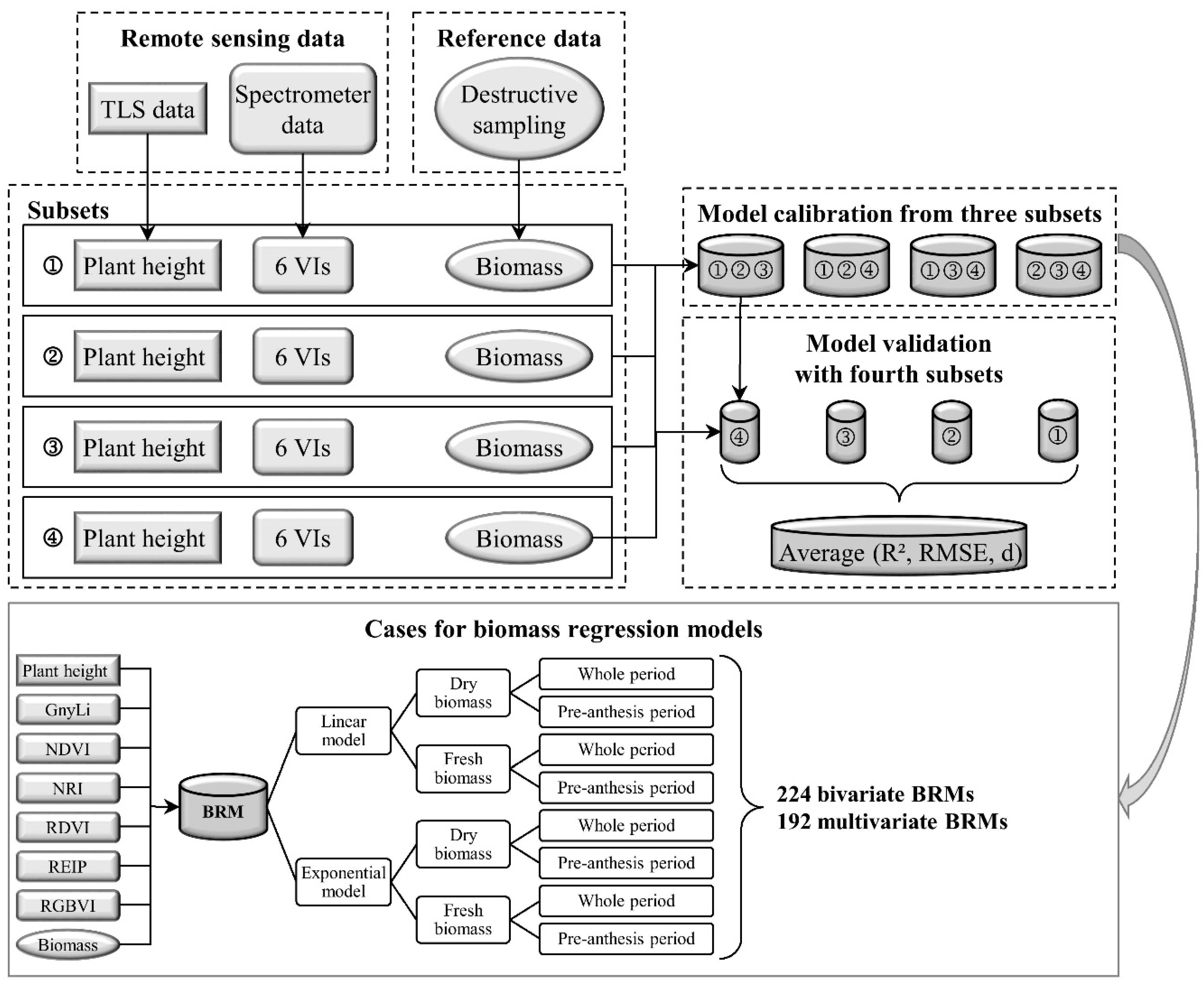
The overall aim of this study was to evaluate whether the fusion of PH and VIs can improve the predictability of dry and fresh barley biomass compared to each parameter as individual estimator. For this work, the use of TLS to derive PH was verified and bivariate BRMs based on PH or one of six VIs as well as multivariate BRMs based on the fusion of PH with each VI were established. Extensive fieldwork over three years supported the practical application of the presented methods for monitoring crop development on plot level. The same instruments were used for all measurements whereby variations through different sensors could be excluded. However, the design of the field experiment and the measurement program was slightly modified and optimized over the years. Hence, only a part of the acquired data was used for the final model generation in order to ensure the comparability between the data sets. In the following, first the retrieval of PH from TLS data is discussed before the different BRMs are examined.

4.1. TLS-Derived Plant Height

The presented study verified the reliability of the laser scanner Riegl LMS-Z420i for capturing crop surfaces. In comparison with past studies [31,43], the scanning angle to the field was optimized through the elevated position on the hydraulic platform. However, uncertainties still remain about the influence of the scanning angle and the fixed position of the scanner during the measurements. As maintained by Ehlert and Heisig [62]—the scanning angle can cause overestimations in the height of reflection points and should be considered in the calculation of heights. In this study, the crop surface was determined from the merged and cleaned point clouds of four scan positions, filtered with a scheme for selecting maximum points. Overestimations should therefore be precluded.
For the practical implementation of CSM-derived plant height measurements, further aspects have to be considered. Usually, the factors time and cost have a major influence on choosing a system. As shown by Hämmerle and Höfle [63] the appropriate point density for generating a CSM varies depending on the application. In further studies, cost-efficient systems, such as the Velodyne HDL-64E [64], should be considered to investigate their potential for capturing crop surfaces in an adequate resolution. In the distant future, low-cost stationary systems might get permanently established for monitoring plant growth on field level. Moreover, recent developments have brought up new laser scanning platforms that might accelerate the field measurement process and optimize the scanning angle. First, ground-based mobile laser scanning (MLS) systems [65] should be taken into account for increasing the homogeneous distribution in the point cloud and thus enhancing a uniform field coverage. Second, unmanned aerial vehicles (UAVs), such as the recently introduced Riegl RiCOPTER [66], should be examined as a potential platform of a light-weight airborne laser scanning (ALS) systems. Promising results have already been achieved for measuring tree heights [67] or detecting pruning of individual stems [68] with UAV-based laser scanning. However, as examined in a comparative study for TLS and common plane-based ALS, the scanning angle and possible resolution influence the results [69] and thus have also to be taken into account for studies on UAV-based scanning systems.
In this study, TLS measurements were used to derive 3D information of points. As shown in other studies, captured intensity values could be used for qualitative analyses of the points, such as detecting single plants [70,71]. Whilst such analyses were not an object of this study they should be considered for further investigations. Moreover, full waveform analysis, commonly known from ALS, can simplify the distinction between laser returns on canopy and ground returns in TLS data [72,73]. The scanner used in this study however is not capable of capturing the full waveform.
The maps of plant height demonstrate the potential of the present approach for deriving plant height information on plot level in a very high resolution. The methodology of spatial plant height mapping can be scaled to field level, as long as the maximum range of the scanner is regarded and the point density is above the required minimum. As shown by Hämmerle and Höfle [63], the coverage of the field and attained mean heights are influenced by the point density. The approach of pixel-wise calculating plant height from TLS-derived CSMs has already shown good results at the field level for monitoring a maize field, about 80 m by 160 m in size [74] and a sugar beet field, about 300 m by 500 m in size [43] captured from four and eight scan positions, respectively. Further studies are necessary for determining crop- or case-specific minimum values for the point density. In this context, the used sensor and its maximum range influence the required number of scan positions.
Nevertheless, for this study, high coefficients of determination between averaged CSM-derived and manual measured plant heights validate the TLS measurements. For the absolute values, differences between the measurement methods have to be considered. Whereas for the manual measurement the heights of ten plants were averaged per plot, the CSM captured the entire crop surface. Consequently, differences in the mean heights occurred, which make precision analysis between TLS data and manual measurements infeasible. The precision of TLS measurements for agricultural applications is presumed from other studies [26,71]. It is important to note that a key advantage of the TLS data is that while plants for the manual measurements are subjectively selected, CSMs enable an objective assessment of spatially continuous plant height.

4.2. Biomass Estimation from Plant Height

Generally, PH performed well for the estimation of biomass in the pre-anthesis and the whole observed period. For dry biomass, PH was the best predictor for the whole observed period and similar good predictor as the best performing VIs for the pre-anthesis. However, PH performed far better for dry biomass than for fresh biomass, although these values are only distinguished by the water content of the sample. Thus, a possible explanation is the fact that the water content is not only influenced by the changing plant phenology across the growing season, but also by varying weather conditions. Moreover, during each day the available soil water and transpiration conditions vary. Hence, the amount of fresh biomass might vary more between the campaigns while the dry biomass is less influenced. Since PH is hardly affected by the water content of the plants, the varying water content in the fresh biomass adds noise to the BRM based on PH which results in lower R2 values.

4.3. Biomass Estimation from Vegetation Indices

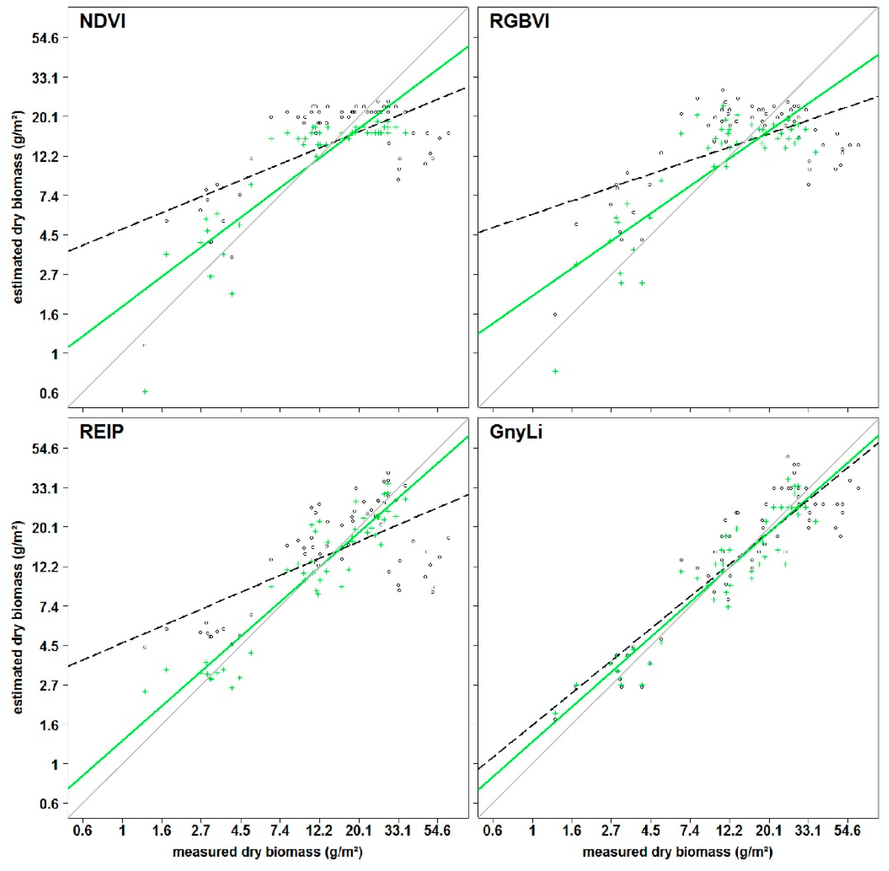
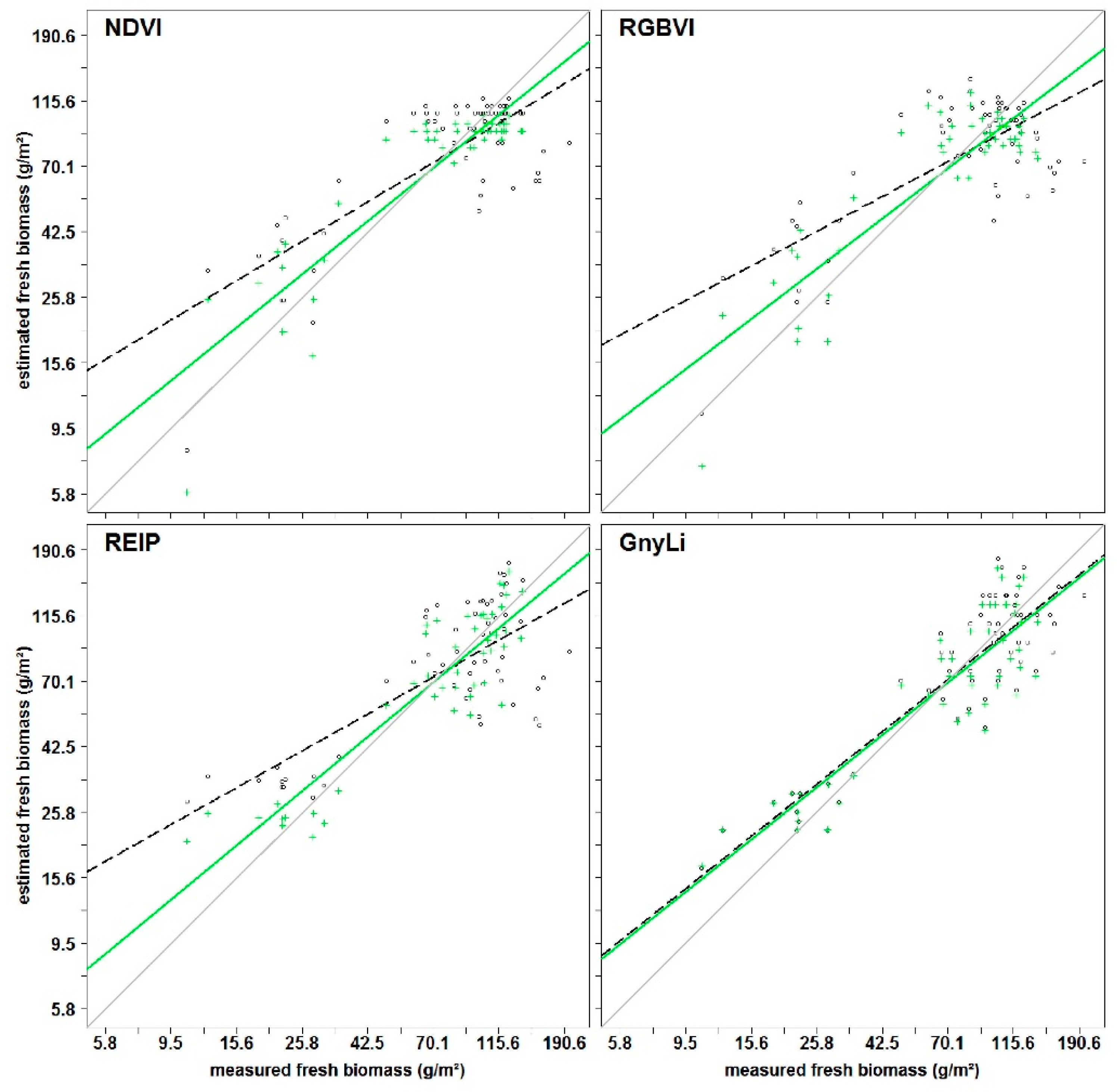
All VIs in this study have previously shown a relationship with biomass and LAI. Since the VIs use different bands within the spectral range, they were subdivided into three categories VIS VIs (RGBVI), VISNIR VIs (NDVI, RDVI, REIP), and NIR VIs (NRI, GnyLi). The VIs showed varying performances for the estimation of dry and fresh biomass, also depending on the regarded time frame of the growing season. Generally, the VIs within a category showed a similar behavior.
The saturation problem of the NDVI type VISNIR VIs was confirmed: Typically, crops reach 100% canopy cover around mid-vegetative phase. However, most crops continue to accumulate biomass and LAI afterwards. At a LAI of about 2.5–3, the absorbed amount of red light reaches a peak while the NIR scattering by leaves continues to increase. Thus, the ratio of NDVI type VISNIR VIs will only show slight changes [13]. In this study, the sensitivity thresholds were about 7.4 g/m² and 55 g/m² for dry and fresh biomass, respectively. Additionally, after heading the canopy de-greens due to flowering and fruit development (after BBCH 5, Table 2). This leads to an increased reflectance in the red part of the spectrum and thus, decreases values of the VISNIR VIs, while the biomass does not decrease. Herein, this discrepancy resulted in an inadequate model parameterization for the BRMs of the VISNIR VIs and poorer results for the whole observed period than for pre-anthesis.
A similar behavior was observable for the RGBVI. The inferior results might be explained by the fact that this VI does not take the reflectance in the NIR region into account, where most of the absorption features for biomass-related plant compounds are situated [75]. These results align well with the ones presented by Bendig et al. [54], where low correlations were found for the RGBVI with biomass after booting stage (BBCH 4, Table 2). In pre-anthesis, relationships of the RGBVI with dry and fresh biomass were similar. These results suggest that the RGBVI is mostly related with vegetation cover and not directly with biomass.
In contrast, NIRVIs, such as GnyLi and NRI, use bands only in the NIR and are thus not affected by the absorption in the red part of the spectrum, which could explain the overall more consistent and better performance of the NIR VIs, particularly after anthesis. A later saturation of these VIs aligns well with other studies [53,56]. Similarly, the REIP did not show any saturation effects in the pre-anthesis and yielded very good results for dry and fresh biomass. These findings can be explained by the major influence of the NIR bands that are not normalized as they are in the NDVI type VIs. Thus, the REIP saturated later than the VISNIR and VIS VIs. Nevertheless, across the whole observed period, the performance of the REIP also decreased due to saturation. The importance of the NIR domain for biomass estimation aligns with other studies [15,16,53,56] and should be further investigated. Similar to PH, the NIR VIs performed better for dry than for fresh biomass while the VISNIR VIs generally performed better with fresh biomass. This suggests that the VISNIR VIs respond more to the canopy water content and the related reflectance change in the NIR shoulder rather than directly to the biomass.
Overall, the results show that the NIR VIs perform best in the prediction of fresh and dry biomass. Moreover, the results indicate that the VIS and VISNIR VIs might not be directly related to biomass. However, no rigorous sensitivity analysis was carried out in this study but, as indicated by the results, such analyses should be carried out in the future.
In general, hyperspectral field measurements have been shown to be useful in earlier studies to estimate biomass [14,15,16,17]. However, VIs are prone to errors by illumination changes [76] and multiangular reflection effects [77]. So far, the influence of these effects on the estimation of plant parameters have not been comprehensively investigated and should be examined for evaluating the potential of VIs for plant parameter estimations. Moreover, ground-based spectrometer measurements are laborious and time-consuming. Automated platforms are under development in different fields of remote sensing to overcome this difficulty but they have not yet become standard. Kicherer et al. [78] developed a robotic platform for phenotyping grapevine based on automatic image acquisition. Results of a mobile multi-sensor phenotyping platform for phenotyping of winter wheat are presented by Kipp et al. [79]. Moreover, hyperspectral UAV-based systems showed promise [55,80,81,82,83]. Unfortunately, the promising NIR domain is currently not well covered by UAV sensing systems.

4.4. Biomass Estimation with Fused Models

Leaves make up a major part of the biomass, and VIs related to biomass are often also responsive to LAI [13,84]. Thus, it was assumed that the spectral information would complement the PH information by adding information about the canopy density and cover.
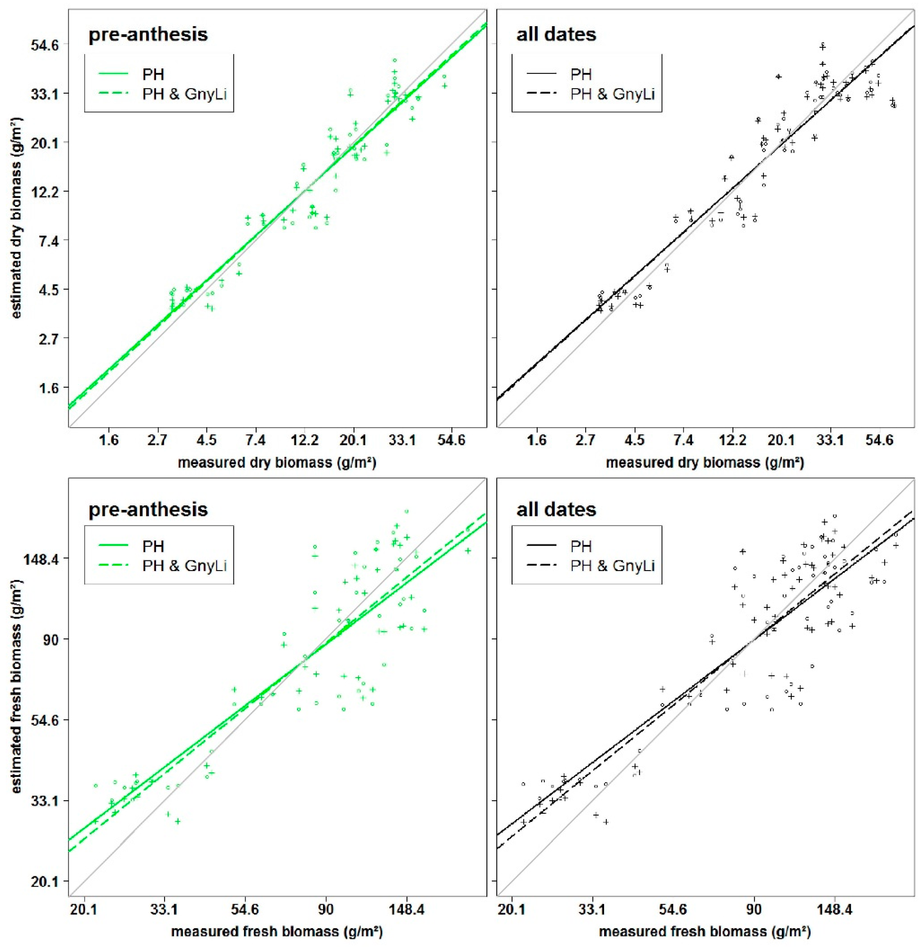
As described above, PH and VIs showed varying performances in the estimation of fresh and dry biomass and for pre-anthesis or the whole observed period. For dry biomass in pre-anthesis, the NIR VIs performed slightly better than PH. Here, the fusion with all VIs improved the predictability, whereby the NIR and VISNIR VIs yielded the best results. This can be explained by the sensitivity of the VIs to the vegetation cover in early growth stages. For the whole observed period, PH clearly outperformed the VIs in the multivariate BRMs and only the fusion with the NIR VIs increased the predictability slightly compared to PH alone. For the VIS and VISNIR VIs, the above described saturation effects might have counteracted the positive effect of the vegetation cover estimation in the early growth stages. Additionally, for pre-anthesis and across the whole observed period, the multivariate BRMs performed similarly regardless which VI was used. This indicates that most of the prediction power can be accounted to PH.
For fresh biomass across the whole observed period, the NIR VIs performed best, followed by PH. Although the VISNIR VIs did not perform well in the bivariate BRMs, they could improve the results when fused with PH. As described above, VISNIR VIs respond to the water content. Thus, they might have complement the PH information for the estimation of fresh biomass. Still, only a slight improvement was achieved with the fused models compared to the NIR VIs alone and overall, the results of multivariate BRMs with different VIs differed only slightly.
In pre-anthesis, only the NDVI and RGBVI performed poorer than PH while the REIP performed best for the fresh biomass. In combination with PH, the results of the NDVI and RDVI were improved the most, while the latter one also achieved the best results of all fused models. For the NIR VIs and REIP none or only very minor improvements were achieved and as for the whole observed period, the water was important because it influences the reflectance in the NIR. Additionally, the VIs correspond to vegetation cover in the early growth stages. Thus, in pre-anthesis already the VIs performed well and PH only rarely contributed to the prediction power. Only the RGBVI, NDVI, and RDVI might have carried complementary information to the PH.
In this study, the NIR VIs showed the overall best performance of the VIs and seemed to carry similar information as PH. Overall, PH and NIR VIs showed the best potential for biomass estimation as individual and fused estimators. This aligns with a recent study by Marshall and Thenkabail [15], in which they have shown the importance of PH and the NIR domain for fresh biomass estimations. The VISNIR VIs seemed to be influenced by the water content and their performance strongly depended on the regarded time frame of the growing season. Although, no comprehensive sensitivity analysis was carried out, these findings align well with other studies [56,85]. Further studies are needed to investigate the influence of the growing stage on the estimation, and whether estimators, which have been found as suitable in across growth stage estimations, are suitable for estimation at individual growth stages. Such in-season estimations are particularly important for applications in precision agriculture. Additionally, in this study VIs known for estimating biomass from hyperspectral data were used. Thus, the full potential of the fusion of 3D spatial and spectral data may not have been explored. Future studies should investigate whether other parts of the spectral range complement PH information better.
Overall, this study demonstrated the strength of bivariate BRMs based on PH and NIR VIs for estimating biomass, with only slight improvements achievable through multivariate models. In contrast, the weak performances of the VIS and VISNIR VIs as individual estimators were compensated through the fusion with PH. However, statements have to be limited, since the models indicated that PH contributed the most to the prediction power. In this context, it has to be noted that neither linear nor exponential models reflected the relation between estimators and biomass perfectly and thus more complex functions have to be considered, which might take the benefits of VIs, like sensitivity to water content, better in to account.
For practical applications the benefit of the fused models might be outweighed by the expenses to deploy two different systems. Referring to this, limitations through the attainable spatial and temporal resolution of each system have to be regarded. As already mentioned, TLS measurements can be scaled up to larger fields, as long as a sufficiently point density can be achieved, which has to be determined crop- and case-specific in further studies. Apart from that, laser scanning appeared as powerful tool for the non-destructive and objective assessment of spatially resolved plant height data. Statements about the accuracy of the measured plant heights are hardly possible due to the already mentioned different spatial resolution of the plant height measurements, however the averaged difference of 0.05 m between TLS-derived and manual measured plant heights corroborate the results (Table A1). A main benefit of the field spectrometer measurements is the high credibility of the acquired spectral data, based on a large number of former studies, however the dependence on solar radiation and the small numbers of measurements per regarded spatial area, herein per plot, are the main disadvantages. Consequently, systems are required which are capable to assess larger areas in less time with the same accuracy of the results. Ideally, spatial and spectral information should be acquired directly through one sensor. For example, recently developed sensing systems and techniques allow to create hyperspectral point clouds [86] and hyperspectral digital surface models [83] with only one sensor and thus, derive 3D spatial and hyperspectral information at the same time. Thus, it can be expected that 3D hyperspectral information will become increasingly available and combined analysis approaches should be further developed.

5. Conclusions and Outlook

Continuously conducting a field experiment with different barley cultivars and the related TLS, field spectrometer, and manual measurements enabled the acquisition of an extensive data set. High R² values up to 0.89, between TLS-derived and manual measured plant heights verified the applicability of the presented approach for a pixel-wise calculation of plant height (PH) from high resolution crop surface models (CSMs). Six established vegetation indices (VIs) were used to extract information from the hyperspectral data. Based on PH and VIs, bivariate and multivariate biomass regression models (BRMs) were established, with varying performances. Whereas PH was supported as strong estimator in the bivariate models (R² up to 0.85), VIs showed highly different results (R2: 0.07–0.87). The multivariate models yielded improvements in some cases (R2 up to 0.89), however in most cases PH had the greatest contribution to the prediction power.
Different models appeared best suitable for dry or fresh biomass estimations, also depending on the regarded time frame of the growing season, but in all cases exponential models performed better than the linear ones: For dry biomass, the bivariate BRM with PH showed the best results for the whole observed period (R2 = 0.85), whereas for the pre-anthesis the REIP and the near-infrared (NIR) VIs GnyLi and NRI showed slightly better results than PH (R2 = 0.86, 0.87). Multivariate BRMs from PH and one VI slightly improved the R² values compared to the bivariate BRMs in some cases. For fresh biomass, the bivariate BRMs of the NIR VIs showed the best results for the whole observed period (both R2 = 0.77). For pre-anthesis, the REIP (R2 = 0.82) showed slightly better results that the NIR VIs (both R2 = 0.79). The multivariate BRM could slightly improve the results in some cases. Additionally, it can be noted that also weakly performing VIs, such as the NDVI or RGBVI, improved the estimations slightly when fused with PH in the multivariate BRMs, both for fresh and dry biomass. These results suggest that specific models should be chosen for specific applications, and a fusion of PH and VIs does not always substantially improve the results. Additionally, when PH and VIs are fused, the choice of the VI does not seem critical in all cases.
Altogether, it should be noted that the presented results are a first step towards the fusion of remotely sensed 3D spatial and spectral data for a precise and non-destructive estimation of crop biomass. Other ways of data fusion may further increase the prediction power. Further studies are also necessary to investigate differences between the years, cultivars, and fertilizer treatments. Moreover, as already mentioned, in-season biomass estimations are important for precision agriculture. Therefore models should be established based on data sets from only one campaign to investigate the potential for timely monitoring and in-season estimations. Accurate and rapidly ascertainable estimations in a high spatial resolution during the growing season could support spatially resolved nitrogen nutrition index calculations. Thereby in-field variations can be considered for optimizing fertilizer application and shrinking the gap between potential and current yield. The fusion of 3D spatial and spectral data might improve such calculations as weaknesses and limitations of one estimator might be compensated through the other one.
With regard to the application in the field, the usability of new platforms should be further investigated. UAV-based light-weight ALS systems reveal potential for vegetation mapping. Futhermore, new technologies like hyperspectral snapshot camera systems which enable the derivation of 3D spatial and hyperspectral information at the same time carry great potential for agricultural applications. Combined with estimation models based on structural and spectral and information, such approaches can become a powerful tool for applications in precision agriculture and biomass monitoring.

Acknowledgments

We would like to thank Dirk Hoffmeister for his knowledgeable support of the TLS measurements and Martin Gnyp for his expertise and effort in collecting the spectral data. Further we extend our thanks to the student assistants for their great work in the field and during the post-processing (Simon Bennertz, Jonas Brands, Janis Broscheit, Markus Drahs, Silas Eichfuss, Sven Ortloff, Maximilian Willkomm), the staff of the Campus Klein-Altendorf for carrying out the experiment (Bernd Bünten, Winfried Bungert, Georg Völkering, Helmut Rehkopf), and the collaborators at the Forschungszentrum Jülich for supporting the laboratory work (Uwe Rascher, Edelgard Schölgens, Mark Müller-Linow, Francisco Pinto). Agim Ballvola is acknowledged for the coordination of the CROP.SENSe.net research group barley. We thank the anonymous reviewers for their valuable comments and Anne Wegner and Lesley-Anne Weiling for the English editing of the manuscript. Helge Aasen was supported by the Grant No. GSGS-2015B-F01 of the Graduate School of Geosciences, University of Cologne during the preparation of this manuscript. This work was carried out within the CROP.SENSe.net project in context of the Ziel 2-Programms NRW 2007–2013 “Regionale Wettbewerbsfähigkeit und Beschäftigung”, financially supported by the Ministry for Innovation, Science and Research (MIWF) of the state North Rhine Westphalia (NRW) and European Union Funds for regional development (EFRE) (005-1103-0018).

Author Contributions

Nora Tilly and Helge Aasen were responsible for the TLS and spectrometer measurements, respectively. The post-processing of the TLS data was carried out by Nora Tilly. Helge Aasen and Georg Bareth selected the used vegetation indices. Nora Tilly substantially designed and established the analysis and mainly wrote this article. Helge Aasen carried out large parts of the analysis and added extensive sections to the manuscript. The research was directed by Georg Bareth, who supervised the whole acquiring, analyzing, and writing process.

Appendix

Table A1. Statistics for the plot-wise averaged CSM-derived and manual measured plant heights (n: number of samples; X ¯ : mean value; min: minimum; max: maximum; SD: standard deviation).
CSM-Derived Plant Height (m)Manual Measured Plant Height (m)
BBCHN leveln X ¯ minmaxSD X ¯ minmaxSD
2012
1N/A40180.150.060.220.040.200.150.250.03
80180.180.140.240.030.200.150.260.03
23040180.210.130.280.040.350.280.420.05
80180.270.200.350.040.350.300.420.04
34940160.580.470.720.080.630.520.800.09
80150.640.480.800.110.660.540.790.08
4N/A40140.730.610.810.060.860.740.960.06
80140.810.710.920.060.890.801.000.06
2013
21840180.210.050.370.090.190.140.250.03
80180.11−0.070.250.080.200.160.270.03
33040180.330.150.510.110.290.190.560.09
80180.250.010.400.110.280.170.450.08
44140180.570.330.830.170.520.390.700.09
80180.560.240.790.180.570.310.810.13
55740160.840.641.110.130.770.660.950.07
80160.790.581.040.120.810.540.940.11
66840140.780.650.970.090.770.660.840.05
80140.770.660.900.080.830.761.000.06
78140140.750.620.960.100.720.650.820.06
80140.720.620.830.070.790.670.890.07
2014
22940180.160.120.240.030.190.120.300.04
80180.180.150.250.030.180.130.270.04
33140180.410.360.510.040.380.310.520.05
80180.420.340.520.050.360.270.450.05
44940180.630.530.700.040.590.530.650.03
80180.630.570.700.040.570.510.640.04
55640180.800.690.870.040.780.680.850.04
80180.810.750.930.040.780.720.890.04
67440180.760.660.840.040.770.680.830.03
80180.790.730.850.030.750.710.820.03
Table A2. Ratio between model calibration and validation ( R c a l 2 : coefficient of determination from calibration; R v a l 2 : coefficient of determination from validation).
Bivariate BRMsMultivariate BRMs
Whole PeriodPre-AnthesisWhole PeriodPre-Anthesis
Estimator R c a l 2 / R v a l 2 R c a l 2 / R v a l 2 Estimatora R c a l 2 / R v a l 2 R c a l 2 / R v a l 2
Dry biomassLinearPH0.980.95
GnyLi0.960.94GnyLi1.000.97
NDVI1.000.89NDVI0.970.95
NRI0.980.95NRI0.980.96
RDVI1.000.95RDVI0.960.95
REIP0.800.85REIP1.000.95
RGBVI1.250.93RGBVI0.970.95
ExponentialPH0.990.99
GnyLi1.000.99GnyLi0.990.99
NDVI1.031.03NDVI1.001.01
NRI1.001.00NRI1.001.00
RDVI1.031.03RDVI1.001.00
REIP0.930.94REIP0.990.97
RGBVI1.051.00RGBVI1.001.01
Fresh biomassLinearPH0.880.86
GnyLi0.890.86GnyLi0.900.86
NDVI0.930.82NDVI0.900.86
NRI0.910.86NRI0.900.86
RDVI0.920.85RDVI0.900.86
REIP0.730.71REIP0.900.82
RGBVI1.050.90RGBVI0.920.90
ExponentialPH0.960.96
GnyLi0.990.96GnyLi0.970.96
NDVI1.051.02NDVI0.991.00
NRI1.000.97NRI0.970.97
RDVI1.041.01RDVI0.990.99
REIP0.870.87REIP0.940.90
RGBVI1.061.04RGBVI1.011.03
a each fused with PH.

Conflicts of Interest

The authors declare no conflict of interest.

References

  1. Mulla, D.J. Twenty five years of remote sensing in precision agriculture: Key advances and remaining knowledge gaps. Biosyst. Eng. 2012, 114, 358–371. [Google Scholar] [CrossRef]
  2. Atzberger, C. Advances in remote sensing of agriculture: Context description, existing Operational Monitoring Systems and Major Information Needs. Remote Sens. 2013, 5, 949–981. [Google Scholar] [CrossRef]
  3. Liaghat, S.; Balasundram, S.K. A Review : The role of remote sensing in precision agriculture. Am. Soc. Agric. Biol. Eng. 2010, 5, 50–55. [Google Scholar] [CrossRef]
  4. Van Wart, J.; Kersebaum, K.C.; Peng, S.; Milner, M.; Cassman, K.G. Estimating crop yield potential at regional to national scales. F. Crop. Res. 2013, 143, 34–43. [Google Scholar] [CrossRef]
  5. UNFPA State of World Population 2010-from Conflict and Crisis to Renewal: Generations of Change. Available online: http://www.unfpa.org/sites/default/files/pub-pdf/EN_SOWP10.pdf (accessed on 1 September 2015).
  6. Oliver, M. An overview of precision agriculture. In Precision Agriculture for Sustainability and Environmental Protection; Oliver, M., Bishop, T., Marchant, B., Eds.; Routledge: London, UK, 2013; pp. 3–19. [Google Scholar]
  7. Fischer, R.A. Irrigated spring wheat and timing and amount of nitrogen fertilizer. II. Physiology of grain yield response. F. Crop. Res. 1993, 33, 57–80. [Google Scholar] [CrossRef]
  8. Boukerrou, L.; Rasmusson, D.D. Breeding for high biomass yield in Spring Barley. Crop Sci. 1990, 30, 31–35. [Google Scholar] [CrossRef]
  9. Price, C.; Munns, R. Growth analysis: A quantitative approach. In Plants in Action; Munns, R., Schmidt, S., Beveridge, C., Eds.; Australian Society of Plant Scientists, New Zealand Society of Plant Biologists, and New Zealand Institute of Agricultural and Horticultural Science: Australia, 2010; Available online: http://plantsinaction.science.uq.edu.au/content/about (accessed on 8 September 2015).
  10. Bidinger, F.; Musgrave, R.B.; Fischer, R.A. Contribution of stored pre-anthesis assimilate to grain yield in wheat and barley. Nature 1977, 270, 431–433. [Google Scholar] [CrossRef]
  11. Greenwood, D.J.; Gastal, F.; Lemaire, G.; Draycott, A.; Millard, P.; Neeteson, J.J. Growth rate and %N of field grown crops: Theory and experiments. Ann. Bot. 1991, 67, 181–190. [Google Scholar]
  12. Ahamed, T.; Tian, L.; Zhang, Y.; Ting, K.C. A review of remote sensing methods for biomass feedstock production. Biomass Bioenerg. 2011, 35, 2455–2469. [Google Scholar] [CrossRef]
  13. Thenkabail, P.S.; Smith, R.B.; de Pauw, E. Hyperspectral vegetation indices and their Relationships with agricultural crop characteristics. Remote Sens. Environ. 2000, 71, 158–182. [Google Scholar] [CrossRef]
  14. Thenkabail, P.S.; Mariotto, I.; Gumma, M.K.; Middleton, E.M.; Landis, D.R.; Huemmrich, K.F. Selection of hyperspectral narrowbands (HNBs) and composition of hyperspectral twoband vegetation indices (HVIs) for biophysical characterization and discrimination of crop types using field reflectance and Hyperion/EO-1 data. IEEE J. Sel. Top. Appl. Earth Obs. Remote Sens. 2013, 6, 427–439. [Google Scholar] [CrossRef]
  15. Marshall, M.; Thenkabail, P. Developing in situ Non-destructive estimates of crop biomass to address issues of scale in Remote Sensing. Remote Sens. 2015, 7, 808–835. [Google Scholar] [CrossRef]
  16. Aasen, H.; Gnyp, M.L.; Miao, Y.; Bareth, G. Automated hyperspectral vegetation index retrieval from multiple correlation matrices with HyperCor. Photogramm. Eng. Remote Sens. 2014, 80, 785–796. [Google Scholar] [CrossRef]
  17. Gnyp, M.L.; Miao, Y.; Yuan, F.; Ustin, S.L.; Yu, K.; Yao, Y.; Huang, S.; Bareth, G. Hyperspectral canopy sensing of paddy rice aboveground biomass at different growth stages. F. Crop. Res. 2014, 155, 42–55. [Google Scholar] [CrossRef]
  18. Lee, W.S.; Alchanatis, V.; Yang, C.; Hirafuji, M.; Moshou, D.; Li, C. Sensing technologies for precision specialty crop production. Comput. Electron. Agric. 2010, 74, 2–33. [Google Scholar] [CrossRef]
  19. Danson, F.M.; Morsdorf, F.; Koetz, B. Airborne and terrestrial Laser scanning for measuring Vegetation Canopy Structure. In Laser Scanning for the Environmental Sciences; Heritage, G.L., Large, A.R.G., Eds.; Wiley-Blackwell: West Sussex, UK, 2009; pp. 201–219. [Google Scholar]
  20. Zhang, L.; Grift, T.E. A LIDAR-based crop height measurement system for Miscanthus giganteus. Comput. Electron. Agric. 2012, 85, 70–76. [Google Scholar] [CrossRef]
  21. Gebbers, R.; Ehlert, D.; Adamek, R. Rapid Mapping of the leaf area index in agricultural crops. Agron. J. 2011, 103, 1532–1541. [Google Scholar] [CrossRef]
  22. Hosoi, F.; Omasa, K. Estimating vertical plant area density profile and growth parameters of a wheat canopy at different growth stages using three-dimensional portable lidar imaging. ISPRS J. Photogramm. Remote Sens. 2009, 64, 151–158. [Google Scholar] [CrossRef]
  23. Saeys, W.; Lenaerts, B.; Craessaerts, G.; de Baerdemaeker, J. Estimation of the crop density of small grains using LiDAR sensors. Biosyst. Eng. 2009, 102, 22–30. [Google Scholar] [CrossRef]
  24. Hosoi, F.; Omasa, K. Estimation of vertical plant area density profiles in a rice canopy at different growth stages by high-resolution portable scanning lidar with a lightweight mirror. ISPRS J. Photogramm. Remote Sens. 2012, 74, 11–19. [Google Scholar] [CrossRef]
  25. Koenig, K.; Höfle, B.; Hämmerle, M.; Jarmer, T.; Siegmann, B. Comparative classification analysis of post-harvest growth detection from terrestrial LiDAR point clouds in precision agriculture. ISPRS J. Photogramm. Remote Sens. 2015, 104, 112–125. [Google Scholar] [CrossRef]
  26. Lumme, J.; Karjalainen, M.; Kaartinen, H.; Kukko, A.; Hyyppä, J.; Hyyppä, H.; Jaakkola, A.; Kleemola, J. Terrestrial laser scanning of agricultural crops. In The International Archives of the Photogrammetry, Remote Sensing and Spatial Information Sciences 37 (Part B5); Chen, J., Jiang, J., Maas, H.-G., Eds.; Organising Committee of the XXI International Congress for Photogrammetry and Remote Sensing: Beijing, China, 2008; pp. 563–566. [Google Scholar]
  27. Ehlert, D.; Horn, H.-J.; Adamek, R. Measuring crop biomass density by laser triangulation. Comput. Electron. Agric. 2008, 61, 117–125. [Google Scholar] [CrossRef]
  28. Ehlert, D.; Adamek, R.; Horn, H.-J. Laser rangefinder-based measuring of crop biomass under field conditions. Precis. Agric. 2009, 10, 395–408. [Google Scholar] [CrossRef]
  29. Olsoy, P.J.; Glenn, N.F.; Clark, P.E. Estimating sagebrush biomass using terrestrial laser scanning. Rangel. Ecol. Manag. 2014, 67, 224–228. [Google Scholar] [CrossRef]
  30. Tilly, N.; Hoffmeister, D.; Cao, Q.; Huang, S.; Lenz-Wiedemann, V.; Miao, Y.; Bareth, G. Multitemporal crop surface models: accurate plant height measurement and biomass estimation with terrestrial laser scanning in paddy rice. J. Appl. Remote Sens. 2014, 8. [Google Scholar] [CrossRef]
  31. Tilly, N.; Hoffmeister, D.; Cao, Q.; Lenz-Wiedemann, V.; Miao, Y.; Bareth, G. Transferability of models for estimating paddy rice biomass from spatial plant height data. Agriculture 2015, 5, 538–560. [Google Scholar] [CrossRef]
  32. Paulus, S.; Schumann, H.; Kuhlmann, H.; Léon, J. High-precision laser scanning system for capturing 3D plant architecture and analysing growth of cereal plants. Biosyst. Eng. 2014, 121, 1–11. [Google Scholar] [CrossRef]
  33. Paulus, S.; Dupuis, J.; Riedel, S.; Kuhlmann, H. Automated analysis of barley organs using 3D laser scanning: An approach for high throughput phenotyping. Sensors 2014, 14, 12670–12686. [Google Scholar] [CrossRef] [PubMed]
  34. Reddersen, B.; Fricke, T.; Wachendorf, M. A multi-sensor approach for predicting biomass of extensively managed grassland. Comput. Electron. Agric. 2014, 109, 247–260. [Google Scholar] [CrossRef]
  35. Blackburn, G.A. Quantifying chlorophylls and caroteniods at leaf and canopy scales. Remote Sens. Environ. 1998, 66, 273–285. [Google Scholar] [CrossRef]
  36. Torabzadeh, H.; Morsdorf, F.; Schaepman, M.E. Fusion of imaging spectroscopy and airborne laser scanning data for characterization of forest ecosystems—A review. ISPRS J. Photogramm. Remote Sens. 2014, 97, 25–35. [Google Scholar] [CrossRef]
  37. Geipel, J.; Link, J.; Claupein, W. Combined spectral and spatial modeling of corn yield based on Aerial Images and Crop Surface Models Acquired with an Unmanned Aircraft System. Remote Sens. 2014, 6, 10335–10355. [Google Scholar] [CrossRef]
  38. Uni Bonn Soil Campus Klein-Altendorf. Available online: http://www.cka.uni-bonn.de/standort/copy_of_boden (accessed on 1 September 2015).
  39. Uni Bonn Climate Campus Klein-Altendorf. Available online: http://www.cka.uni-bonn.de/standort/copy_of_klima (accessed on 1 September 2015).
  40. Meier, U. Growth Stages of Mono- and Dicotyledonous Plants, 2nd ed.; Blackwell: Berlin, Germany, 2001. [Google Scholar]
  41. Lancashire, P.D.; Bleiholder, H.; van den Boom, T.; Langelüddeke, P.; Strauss, R.; Weber, E.; Witzenberger, A. A uniform decimal code for growth stages of crops and weeds. Ann. Appl. Biol. 1991, 119, 561–601. [Google Scholar] [CrossRef]
  42. Riegl LMS GmbH Datasheet Riegl LMS-Z420i. Available online: http://www.riegl.com/uploads/tx_pxpriegldownloads/10_DataSheet_Z420i_03-05-2010.pdf (accessed on 1 September 2015).
  43. Hoffmeister, D.; Bolten, A.; Curdt, C.; Waldhoff, G.; Bareth, G. High resolution Crop Surface Models (CSM) and Crop Volume Models (CVM) on field level by terrestrial laser scanning. Proc. SPIE 2010, 7840. [Google Scholar] [CrossRef]
  44. Topcon Positioning Systems, I. HiPer Pro Operator’s Manual. Available online: http://www.top-survey.com/top-survey/downloads/HiPerPro_om.pdf (accessed on 1 September 2015).
  45. Besl, P.J.; McKay, N.D. A method for registration of 3D shapes. IEEE Trans. Pattern Anal. Mach. Intell. 1992, 14, 239–256. [Google Scholar] [CrossRef]
  46. Johnston, K.; Ver Hoef, J.M.; Krivoruchko, K.; Lucas, N. Using ArcGIS Geostatistical Analyst; ESRI: Redlands, CA, USA, 2001. [Google Scholar]
  47. Rouse, J.W.; Haas, R.H.; Schell, J.A.; Deering, D.W. Monitoring vegetation systems in the great plains with erts. In Third Earth Resources Technology Satellite-1 Symposium; NASA: Washington, DC, USA, 1974; pp. 309–317. [Google Scholar]
  48. Haboudane, D.; Miller, J.R.; Pattey, E.; Zarco-Tejada, P.J.; Strachan, I.B. Hyperspectral vegetation indices and novel algorithms for predicting green LAI of crop canopies: Modeling and validation in the context of precision agriculture. Remote Sens. Environ. 2004, 90, 337–352. [Google Scholar] [CrossRef]
  49. Roujean, J.L.; Breon, F.M. Estimating PAR absorbed by vegetation from bidirectional reflectance measurements. Remote Sens. Environ. 1995, 51, 375–384. [Google Scholar] [CrossRef]
  50. Broge, N.H.; Leblanc, E. Comparing prediction power and stability of broadband and hyperspectral vegetation indices for estimation of green leaf area index and canopy chlorophyll density. Remote Sens. Environ. 2001, 76, 156–172. [Google Scholar] [CrossRef]
  51. Guyot, G.; Baret, F. Utilisation de la haute resolution spectrale pour suivre l’etat des couverts vegetaux. In Proceedings of the 4th International Colloquium on Spectral Signatures of Objects in Remote Sensing, Aussois, France, 18–22 January 1988; pp. 279–286.
  52. Guyot, G.; Baret, F.; Jacquemoud, S. Imaging spectroscopy for vegetation studies. In Imaging Spectroscopy for Vegetation Studies; Toselli, F., Bodechtel, J., Eds.; Kluwer: Dordrecht, The Netherlands, 1992; pp. 145–165. [Google Scholar]
  53. Koppe, W.; Li, F.; Gnyp, M.L.; Miao, Y.; Jia, L.; Chen, X.; Zhang, F.; Bareth, G. Evaluating multispectral and hyperspectral satellite Remote Sensing data for estimating winter wheat growth parameters at regional scale in the North China plain. Photogramm.Fernerkundung Geoinf. 2010, 3, 167–178. [Google Scholar] [CrossRef]
  54. Bendig, J.; Yu, K.; Aasen, H.; Bolten, A.; Bennertz, S.; Broscheit, J.; Gnyp, M.L.; Bareth, G. Combining UAV-based plant height from crop surface models, visible, and near infrared vegetation indices for biomass monitoring in barley. Int. J. Appl. Earth Obs. Geoinf. 2015, 39, 79–87. [Google Scholar] [CrossRef]
  55. Bareth, G.; Aasen, H.; Bendig, J.; Gnyp, M.L.; Bolten, A.; Jung, A.; Michels, R.; Soukkamäki, J. Low-weight and UAV-based hyperspectral full-frame cameras for monitoring Crops: Spectral Comparison with Portable Spectroradiometer Measurements. Photogramm.Fernerkundung Geoinf. 2015, 1, 69–79. [Google Scholar] [CrossRef]
  56. Gnyp, M.L.; Bareth, G.; Li, F.; Lenz-Wiedemann, V.I.S.; Koppe, W.; Miao, Y.; Hennig, S.D.; Jia, L.; Laudien, R.; Chen, X.; Zhang, F. Development and implementation of a multiscale biomass model using hyperspectral vegetation indices for winter wheat in the North China Plain. Int. J. Appl. Earth Obs. Geoinf. 2014, 33, 232–242. [Google Scholar] [CrossRef]
  57. R Development Core Team. The R Project for Statistical Computing. Available online: http://www.r-project.org/ (accessed on 1 September 2015).
  58. Hair, J.F.; Black, W.C.; Babin, B.J.; Anderson, R.E. Multivariate Data Analysis, 7th ed.; Pearson: London, UK, 2010. [Google Scholar]
  59. Willmott, C.J.; Wicks, D.E. An empirical method for the spatial interpolation of monthly precipitation within California. Phys. Geogr. 1980, 1, 59–73. [Google Scholar]
  60. Willmott, C.J. On the validation of models. Phys. Geogr. 1981, 2, 184–194. [Google Scholar]
  61. Tilly, N.; Hoffmeister, D.; Aasen, H.; Brands, J.; Bareth, G. Multi-temporal crop surface models derived from terrestrial laser scanning for accurate plant height measurement and biomass estimation of barley. Kölner Geogr. Arb. 2014, 94, 83–91. [Google Scholar]
  62. Ehlert, D.; Heisig, M. Sources of angle-dependent errors in terrestrial laser scanner-based crop stand measurement. Comput. Electron. Agric. 2013, 93, 10–16. [Google Scholar] [CrossRef]
  63. Hämmerle, M.; Höfle, B. Effects of reduced terrestrial LiDAR point density on high-resolution grain crop surface models in precision agriculture. Sensors 2014, 14, 24212–24230. [Google Scholar] [CrossRef] [PubMed]
  64. Velodyne Velodyne HDL-64E User’s Manual. Avalible Online: http://www.velodynelidar.com/lidar/products/manual/63-HDL64E S2 Manual_Rev D_2011_web.pdf (accessed on 6 September 2015).
  65. Kukko, A.; Kaartinen, H.; Hyyppä, J.; Chen, Y. Multiplatform mobile Laser scanning: Usability and performance. Sensors 2012, 12, 11712–11733. [Google Scholar] [CrossRef]
  66. Riegl LMS GmbH Infosheet RiCOPTER. Avalible Online: http://www.riegl.com/uploads/tx_pxpriegldownloads/RiCOPTER_at_a_glance_2015-03-31.pdf (accessed on 6 September 2015).
  67. Jaakkola, A.; Hyyppä, J.; Kukko, A.; Yu, X.; Kaartinen, H.; Lehtomäki, M.; Lin, Y. A low-cost multi-sensoral mobile mapping system and its feasibility for tree measurements. ISPRS J. Photogramm. Remote Sens. 2010, 65, 514–522. [Google Scholar] [CrossRef]
  68. Wallace, L.; Watson, C.; Lucieer, A. Detecting pruning of individual stems using airborne laser scanning data captured from an Unmanned Aerial Vehicle. Int. J. Appl. Earth Obs. Geoinf. 2014, 30, 76–85. [Google Scholar] [CrossRef]
  69. Luscombe, D.J.; Anderson, K.; Gatis, N.; Wetherelt, A.; Grand-Clement, E.; Brazier, R.E. What does airborne LiDAR really measure in upland ecosystems? Ecohydrology 2014, 8, 584–594. [Google Scholar] [CrossRef] [Green Version]
  70. Hoffmeister, D.; Tilly, N.; Bendig, J.; Curdt, C.; Bareth, G. Detektion von Wachstumsvariabilität in vier Zuckerrübensorten. In Informationstechnologie für eine nachhaltige Landbewirtschaftung, Proc. 32. GIL-Jahrestagung; Clasen, M., Fröhlich, G., Bernhardt, H., Hildebrand, K., Theuvsen, B., Eds.; Köllen Verlag: Bonn, Germany, 2012; pp. 135–138. [Google Scholar]
  71. Höfle, B. Radiometric correction of terrestrial LiDAR point cloud data for Individual Maize Plant Detection. IEEE Geosci. Remote Sens. Lett. 2014, 11, 94–98. [Google Scholar] [CrossRef]
  72. Elseberg, J.; Borrmann, D.; Nüchter, A. Full Wave Analysis in 3D laser scans for vegetation detection in urban environments. In Proceedings of the 2011 XXIII International Symposium on Information, Communication and Automation Technologies, Sarajevo, Yugoslavia, 27–29 October 2011; pp. 1–7.
  73. Pirotti, F.; Guarnieri, A.; Vettore, A. Vegetation filtering of waveform terrestrial laser scanner data for DTM production. Appl. Geomatics 2013, 5, 311–322. [Google Scholar] [CrossRef]
  74. Tilly, N.; Hoffmeister, D.; Schiedung, H.; Brands, J.; Bareth, G.; Conservation, R.; Detection, C. Terrestrial laser scanning for plant height measurement and biomass estimation of maize. ISPRS Int. Arch. Photogramm. Remote Sens. Spat. Inf. Sci. 2014, 1, 181–187. [Google Scholar] [CrossRef]
  75. Kumar, L.; Schmidt, K.; Dury, S.; Skidmore, A. Imaging spectrometry and vegetation science. In Imaging Spectrometry: Basic Principles and Prospective Applications; van der Meer, F., Jong, S.D., Eds.; Springer Netherlands: Dordrecht, The Netherlands, 2001; pp. 111–155. [Google Scholar]
  76. Damm, A.; Guanter, L.; Verhoef, W.; Schläpfer, D.; Garbari, S.; Schaepman, M.E. Impact of varying irradiance on vegetation indices and chlorophyll fluorescence derived from spectroscopy data. Remote Sens. Environ. 2015, 156, 202–215. [Google Scholar] [CrossRef]
  77. Burkart, A.; Aasen, H.; Alonso, L.; Menz, G.; Bareth, G.; Rascher, U. Angular dependency of hyperspectral measurements over wheat characterized by a novel UAV based goniometer. Remote Sens. 2015, 7, 725–746. [Google Scholar] [CrossRef]
  78. Kicherer, A.; Herzog, K.; Pflanz, M.; Wieland, M.; Rüger, P.; Kecke, S.; Kuhlmann, H.; Töpfer, R. An automated field phenotyping pipeline for application in grapevine research. Sensors 2015, 15, 4823–4836. [Google Scholar] [CrossRef] [PubMed]
  79. Kipp, S.; Mistele, B.; Baresel, P.; Schmidhalter, U. High-throughput phenotyping early plant vigour of winter wheat. Eur. J. Agron. 2014, 52, 271–278. [Google Scholar] [CrossRef]
  80. Quemada, M.; Gabriel, J.; Zarco-Tejada, P. Airborne hyperspectral images and ground-level optical sensors as assessment tools for maize nitrogen fertilization. Remote Sens. 2014, 6, 2940–2962. [Google Scholar] [CrossRef]
  81. Suomalainen, J.; Anders, N.; Iqbal, S.; Roerink, G.; Franke, J.; Wenting, P.; Hünniger, D.; Bartholomeus, H.; Becker, R.; Kooistra, L. A lightweight hyperspectral mapping system and photogrammetric processing chain for unmanned aerial vehicles. Remote Sens. 2014, 6, 11013–11030. [Google Scholar] [CrossRef]
  82. Honkavaara, E.; Saari, H.; Kaivosoja, J.; Pölönen, I.; Hakala, T.; Litkey, P.; Mäkynen, J.; Pesonen, L. Processing and assessment of spectrometric, stereoscopic imagery collected using a lightweight UAV spectral camera for precision agriculture. Remote Sens. 2013, 5, 5006–5039. [Google Scholar] [CrossRef] [Green Version]
  83. Aasen, H.; Burkart, A.; Bolten, A.; Bareth, G. Generating 3D hyperspectral information with lightweight UAV snapshot cameras for vegetation monitoring: From camera calibration to quality assurance. ISPRS J. Photogramm. Remote Sens. 2015. accepted. [Google Scholar] [CrossRef]
  84. Thenkabail, P.S.; Smith, R.B.; de Pauw, E. Evaluation of narrowband and broadband vegetation indices for determining optimal hyperspectral wavebands for agricultural crop characterization. Photogramm. Eng. Remote Sens. 2002, 68, 607–621. [Google Scholar]
  85. Gnyp, M.L.; Yu, K.; Aasen, H.; Yao, Y.; Huang, S.; Miao, Y.; Bareth, G. Analysis of crop reflectance for estimating biomass in rice canopies at different phenological stages. Photogramm. Fernerkundung Geoinf. 2013, 4, 351–365. [Google Scholar] [CrossRef]
  86. Vauhkonen, J.; Hakala, T.; Suomalainen, J.; Kaasalainen, S.; Nevalainen, O.; Vastaranta, M.; Holopainen, M.; Hyyppa, J. Classification of spruce and pine trees using active Hyperspectral LiDAR. IEEE Geosci. Remote Sens. Lett. 2013, 10, 1138–1141. [Google Scholar] [CrossRef]

