
Assessing the Suitability of Future Multi- and Hyperspectral Satellite Systems for Mapping the Spatial Distribution of Norway Spruce Timber Volume


 ,
,
Abstract
:
1. Introduction
- Integration of routinely acquired forest resource assessments and spectral information for estimating the spatial distribution of timber volume in managed Norway spruce (Picea abies) forests.
- Identification of sensitive wavelengths for volume estimation in intensively managed Norway spruce forests.
- Assessment of concepts (PLSR vs. k-NN) for producing spatially explicit maps of Norway spruce timber volume within administrative forest units.
- Evaluation of the spectral and spatial resolution characteristics of Sentinel-2 and EnMAP for mapping Norway spruce timber volume.
2. Material and Methods
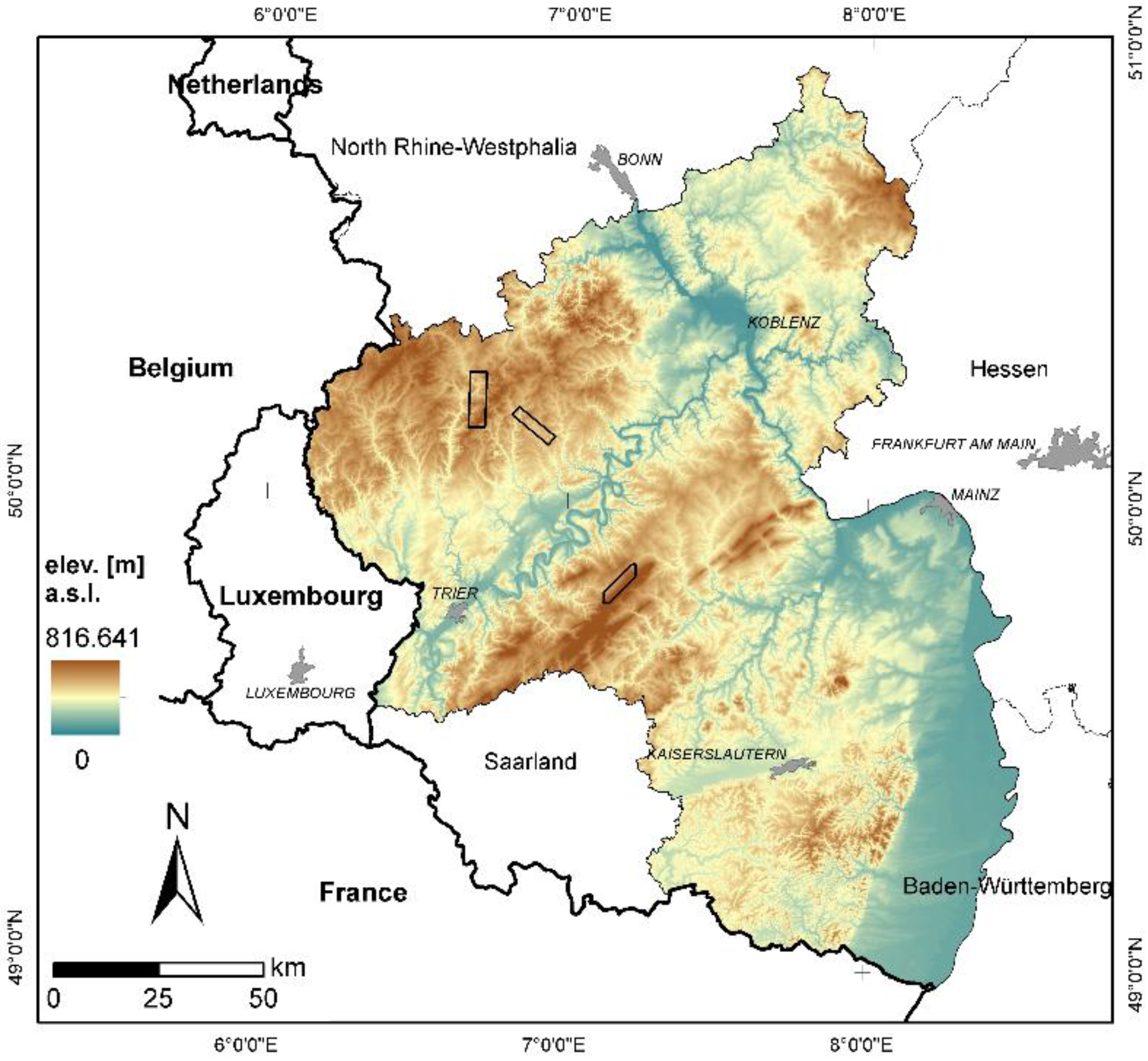
2.1. Study Area

2.2. Data
2.2.1. Airborne HyMap imagery
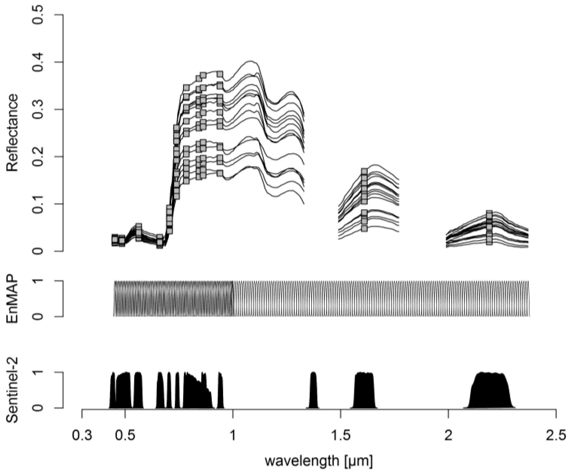
2.2.2. EnMAP and Sentinel-2 Data Simulation
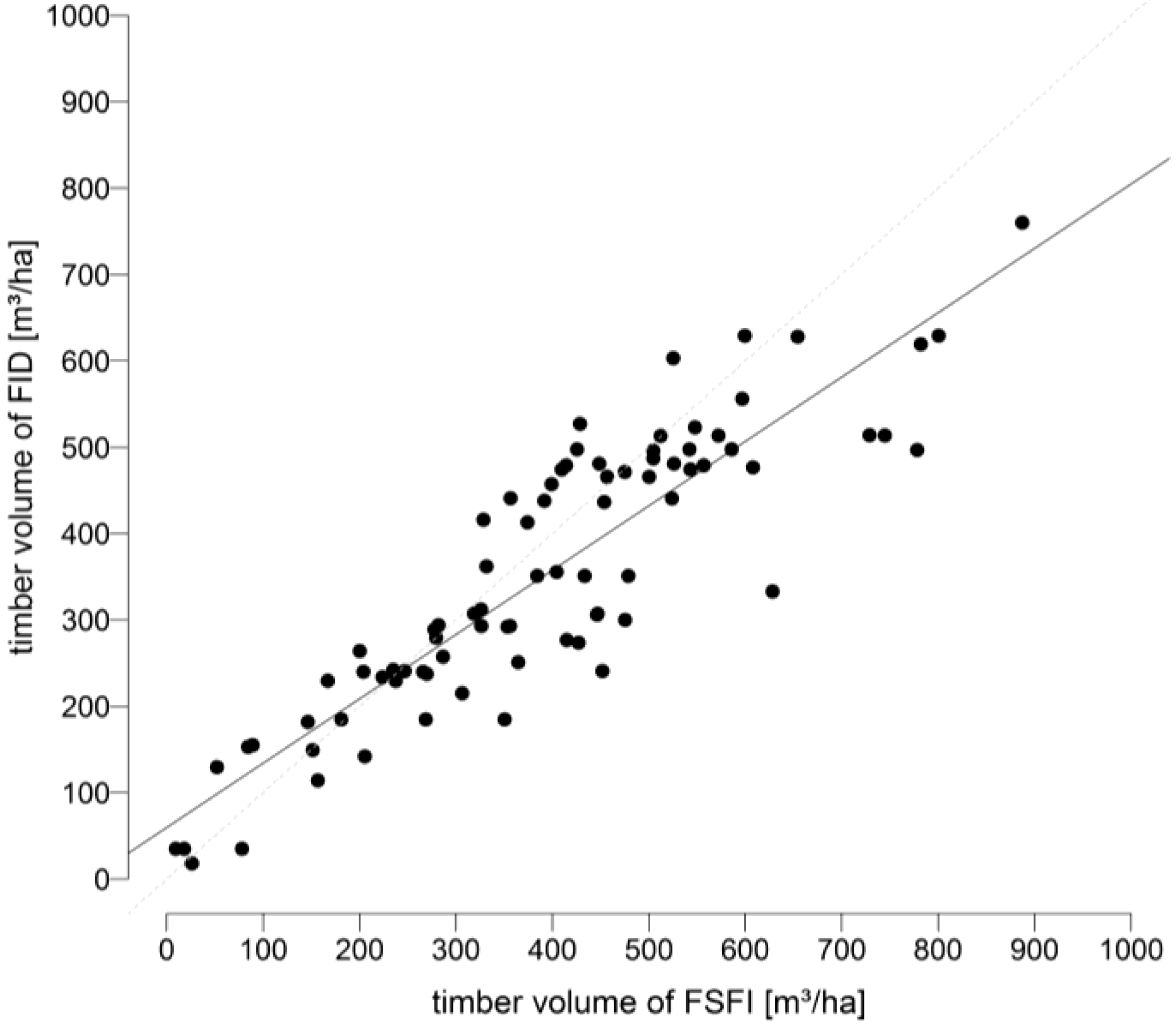
2.2.3. Timber Volume Reference Data

2.3. Methods
2.3.1. Extraction of Spectral References
2.3.2. Reference Data and Identification of Sensitive Spectral Regions
2.3.3. Predictive Modeling
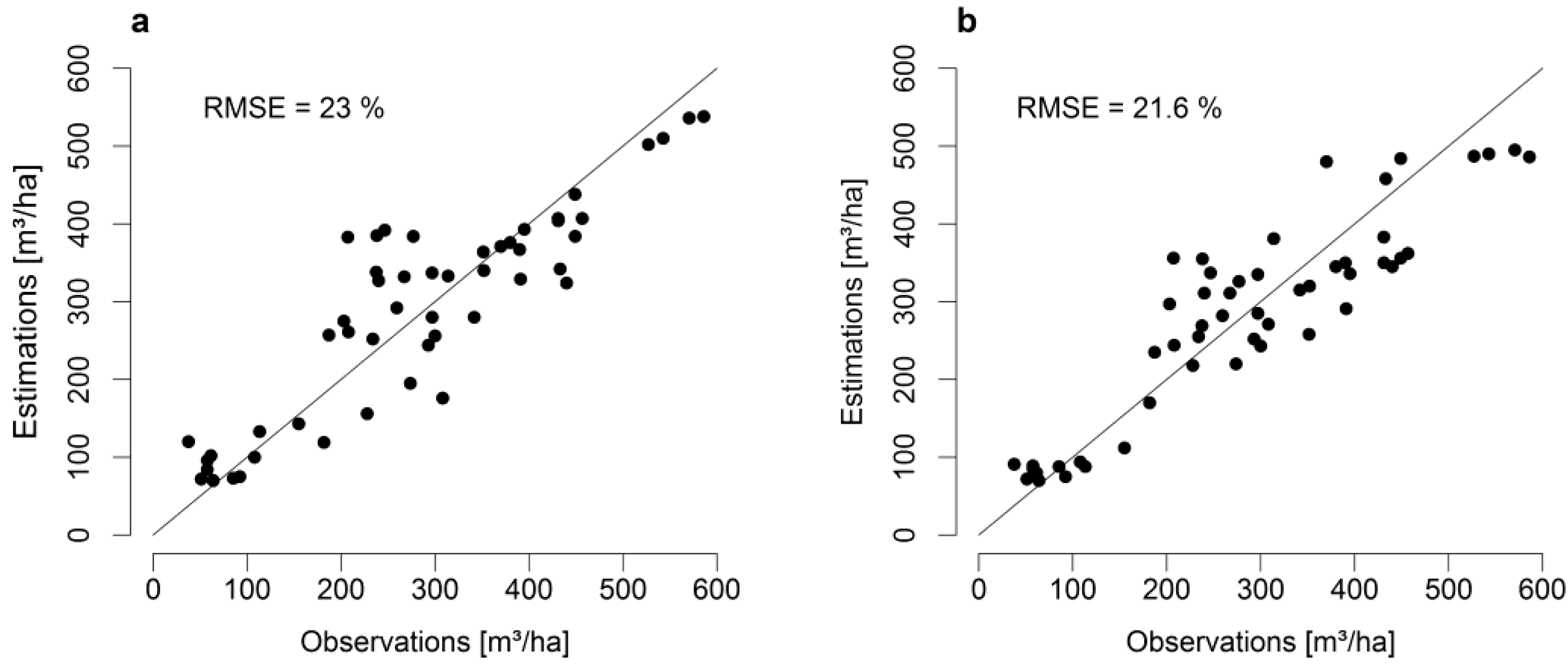
2.3.4. Model Validation
2.3.5. Model Application
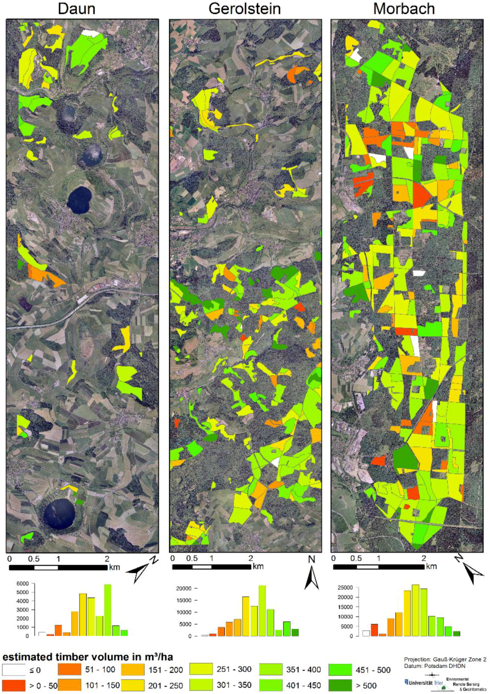
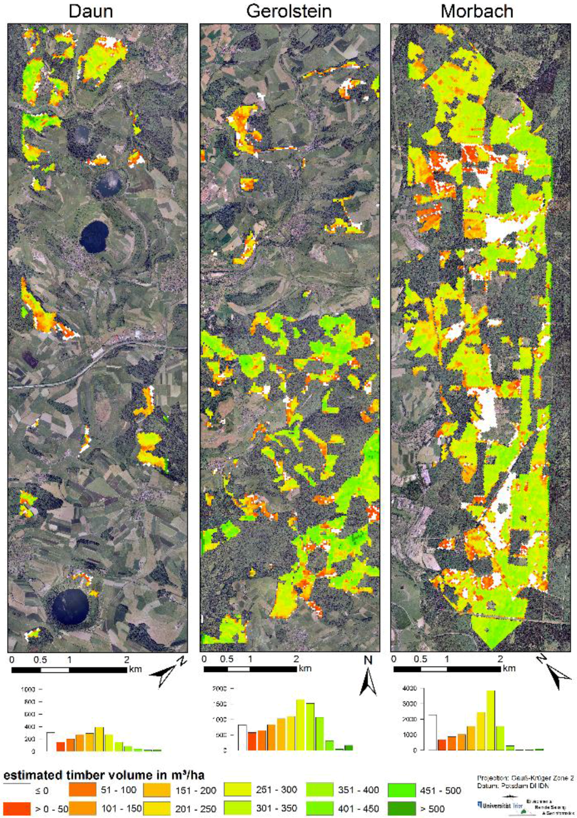
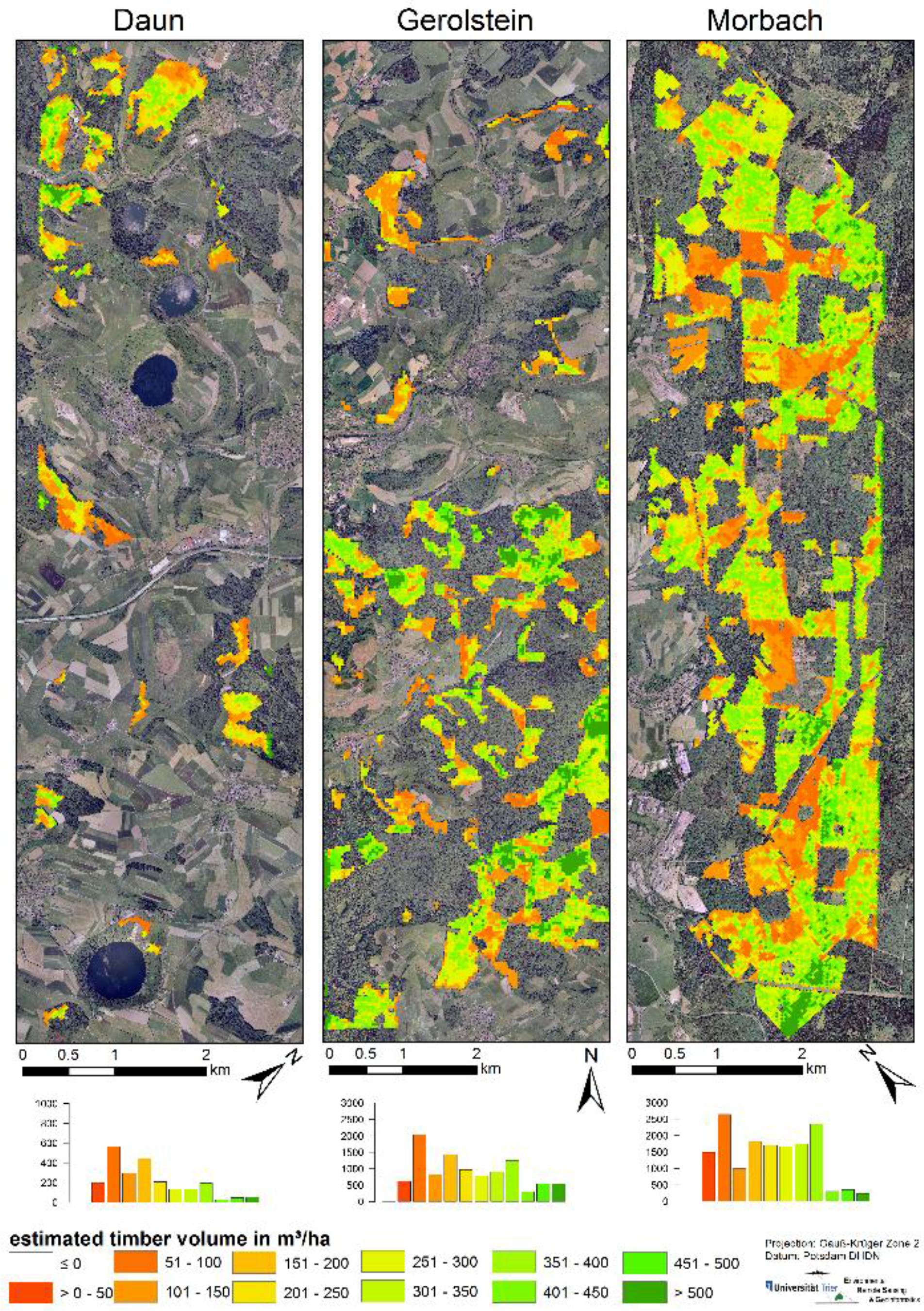
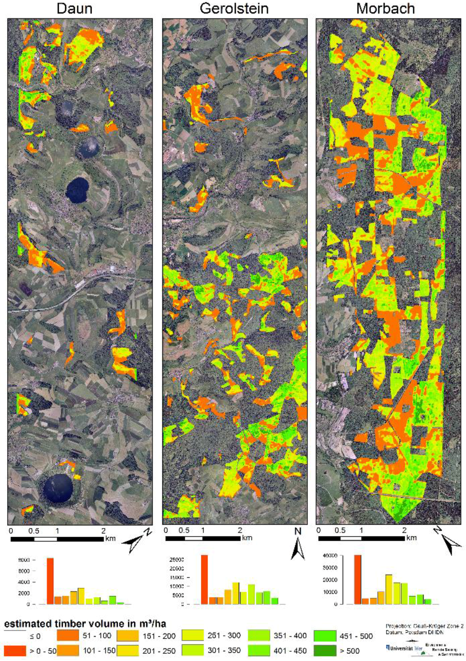
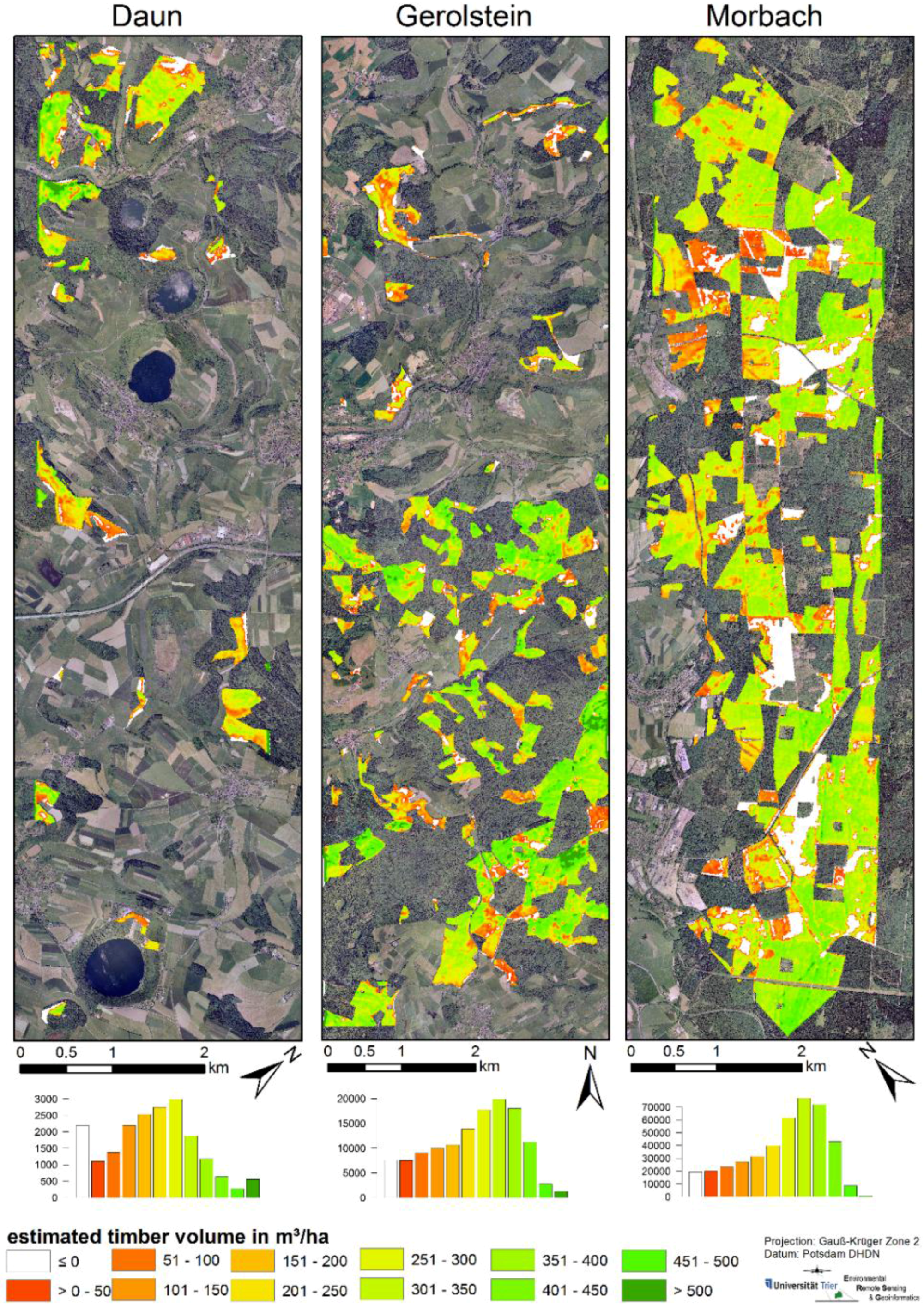
2.3.6. Prediction Maps
3. Results
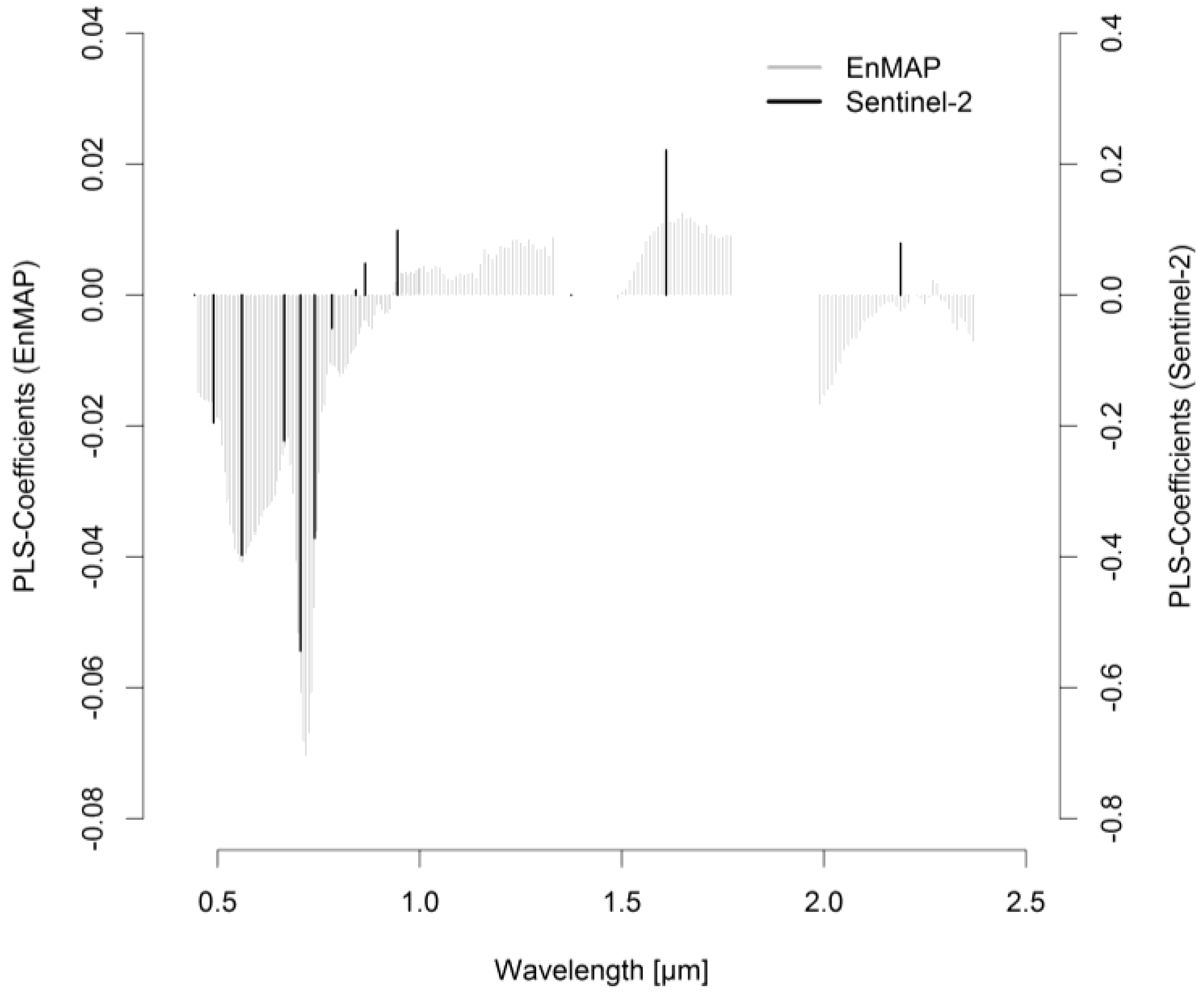
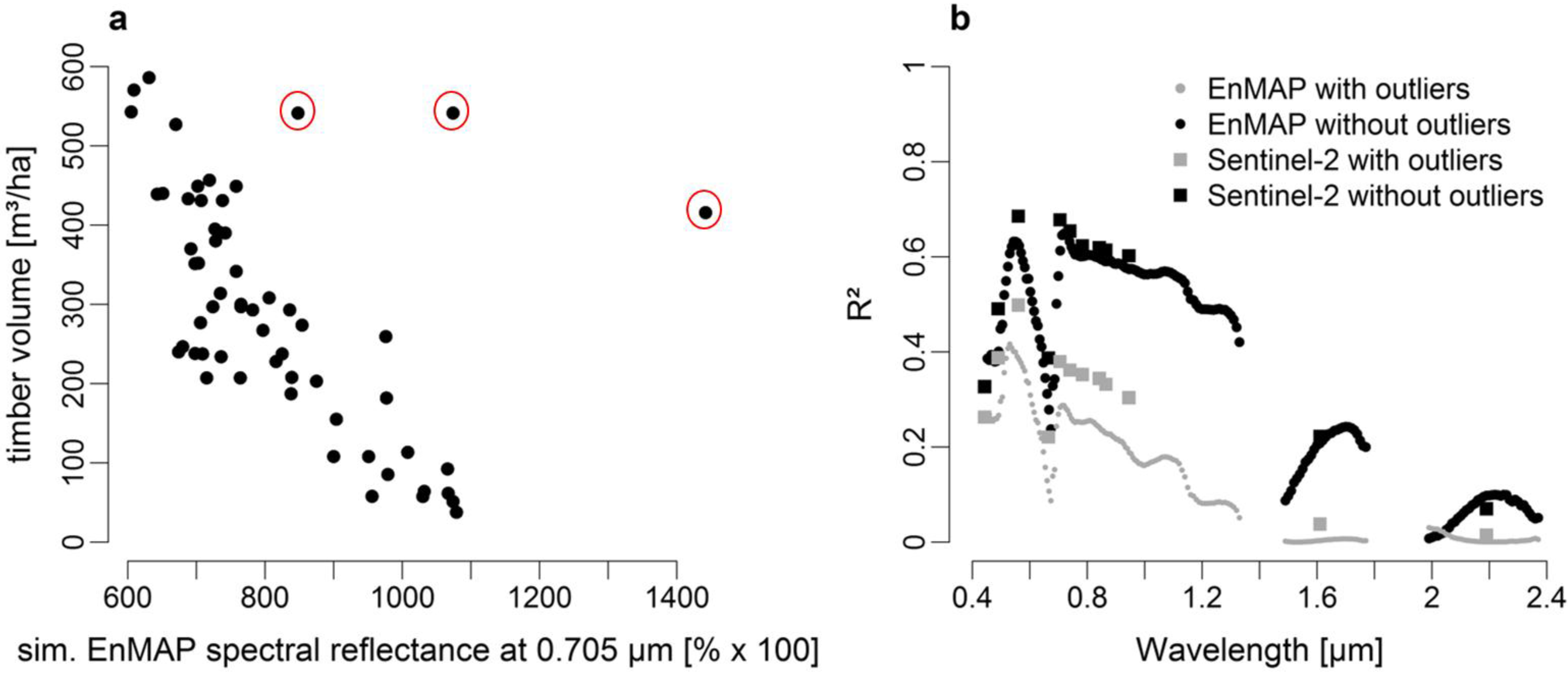
3.1. Identification of Sensitive Spectral Regions

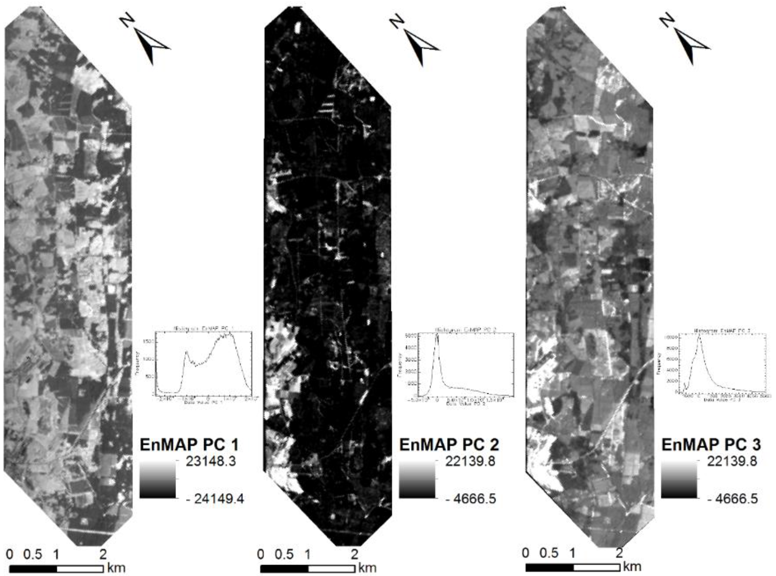
3.2. Principal Component Analysis

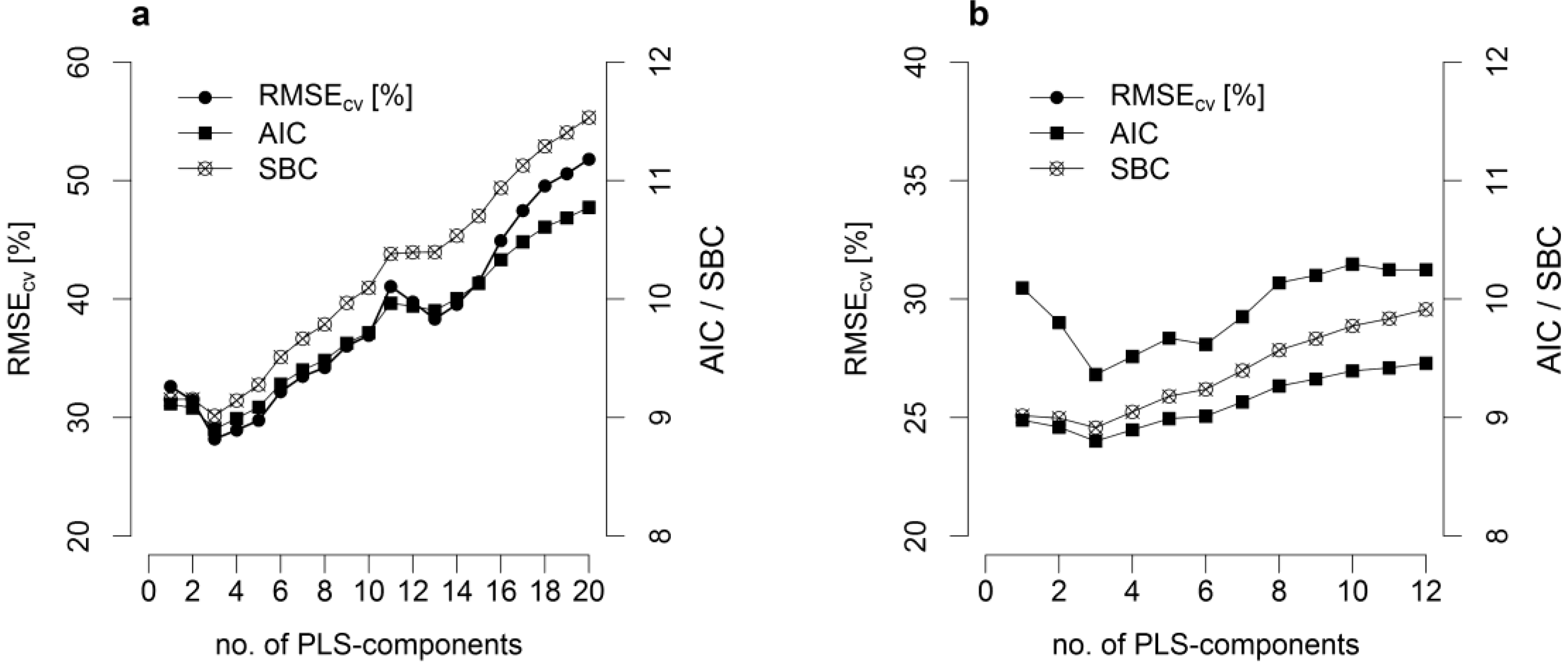
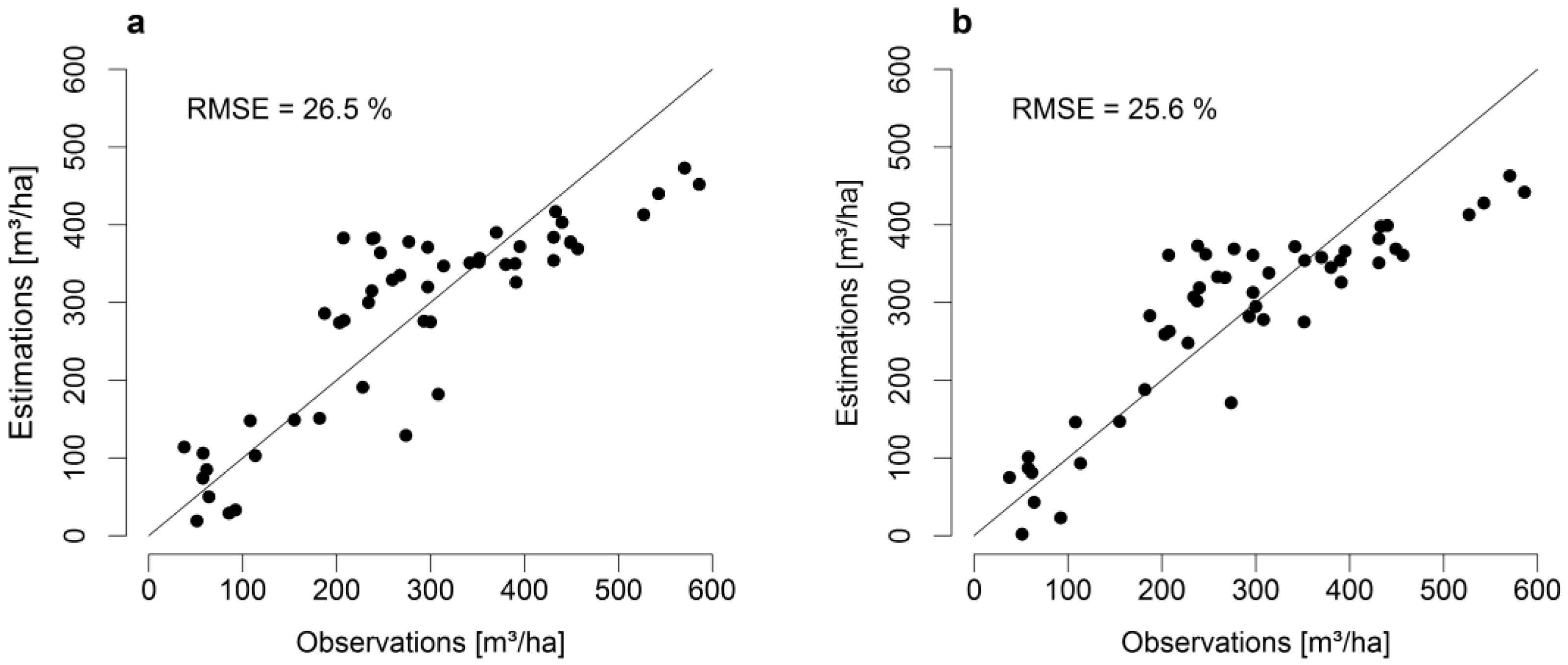
3.3. PLSR

| Estimation | Reference | ||||||
|---|---|---|---|---|---|---|---|
| loo-cv | Administrative Forest Unit | ||||||
| Mean Timber Volume (m³/ha) | Biascv (m³/ha) | RMSEcv (%) | Mean Timber Volume (m³/ha) | Biascv (m³/ha) | RMSEcv (%) | Mean Timber Volume (m³/ha) | |
| PLSR (EnMAP) | 283.61 | –0.08 | 28.19 | 283.63 | –0.06 | 26.48 | 283.69 |
| PLSR (Sentinel-2) | 282.39 | –1.29 | 26.81 | 278.08 | –5.61 | 25.60 | |

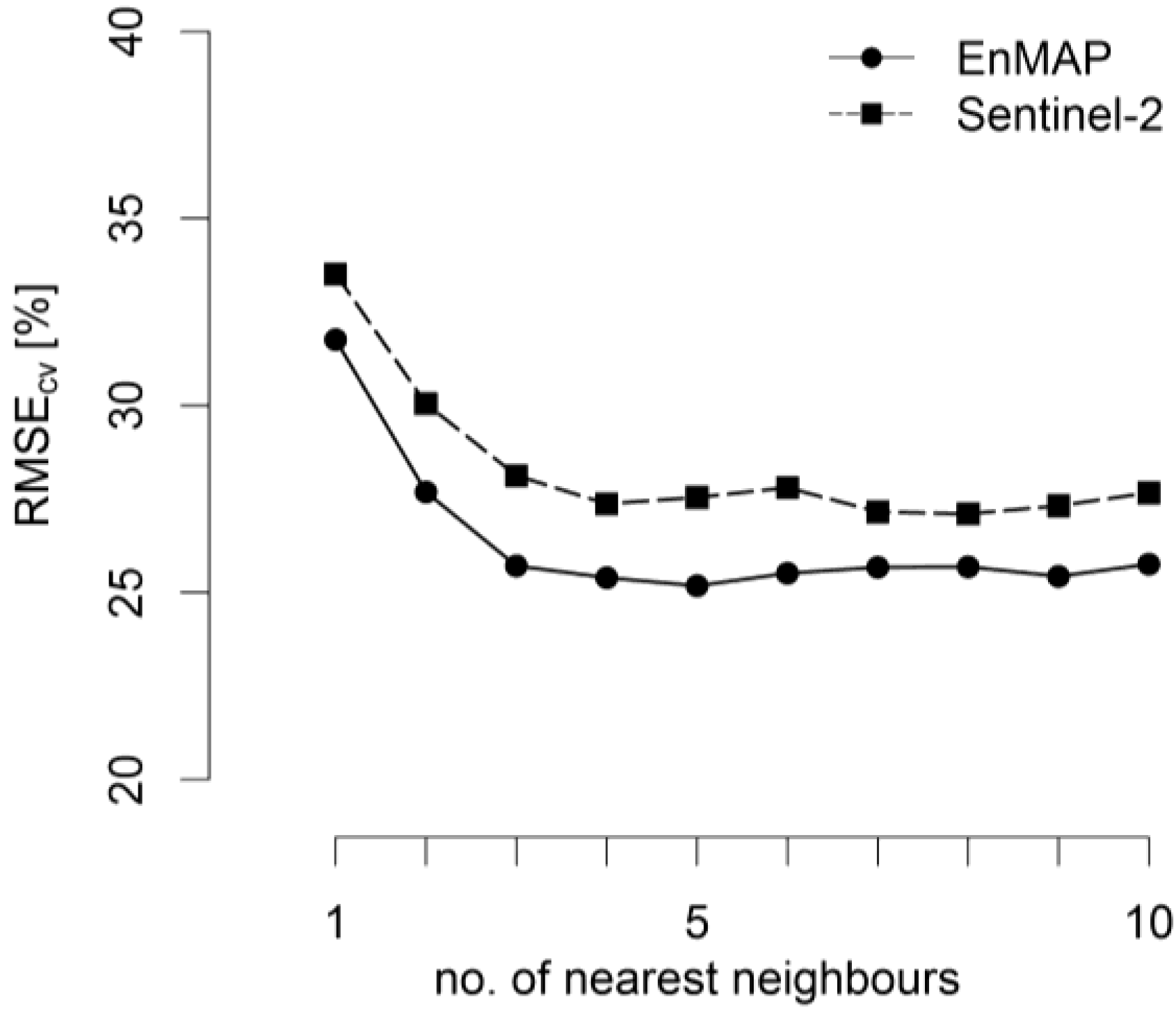
3.4. k-NN
| Principal Component | No. of Nearest Neighbours (k) | RMSEloo-cv (%) | RMSEloo-cv (m³/ha) | |||||
| EnMAP | PC 1 | PC 2 | PC 3 | PC 7 | ||||
| R² | 0.69 | 0.35 | 0.63 | 0.37 | ||||
| feature band weighting | 1 | 4 | 30.22 | 85.72 | ||||
| 1 | 4 | 41.41 | 117.49 | |||||
| 1 | 1 | 3 | 28.49 | 80.81 | ||||
| 1 | 1 | 1 | 3 | 28.48 | 80.80 | |||
| 1 | 1 | 1 | 3 | 28.43 | 80.65 | |||
| 1 | 1 | 1 | 1 | 3 | 28.44 | 80.67 | ||
| optimized feature band weighting | 0.25 | 2 | 3 | 25.70 | 72.93 | |||
| Principal Component | No. of Nearest Neighbours (k) | RMSEloo-cv [%] | RMSEloo-cv [m³/ha] | |||||
| Sentinel-2 | PC 1 | PC 3 | PC 9 | PC 10 | ||||
| R² | 0.68 | 0.69 | 0.27 | 0.28 | ||||
| feature band weighting | 1 | 5 | 32.66 | 92.65 | ||||
| 1 | 3 | 37.27 | 105.73 | |||||
| 1 | 1 | 4 | 28.40 | 80.56 | ||||
| 1 | 1 | 1 | 4 | 28.32 | 80.34 | |||
| 1 | 1 | 1 | 1 | 4 | 28.18 | 79.93 | ||
| optimized feature band weighting | 0.5 | 1.75 | 4 | 27.37 | 77.44 | |||

| LOO-cv | Administrative Forest Unit | Reference | ||||||
|---|---|---|---|---|---|---|---|---|
| Mean Timber Volume (estim.) (m³/ha) | Biascv (m³/ha) | RMSEcv (%) | Mean Timber Volume (estim.) (m³/ha) | Biascv (m³/ha) | RMSEcv (%) | Mean Timber Volume (m³/ha) | ||
| k-NN (EnMAP); k = 3 | 280.16 | –3.53 | 25.7 | 287.33 | 3.64 | 23.11 | 283.69 | |
| k-NN (Sentinel-2); k = 4 | 279.47 | –4.22 | 27.37 | 280.16 | –3.53 | 21.58 | ||
4. Discussion
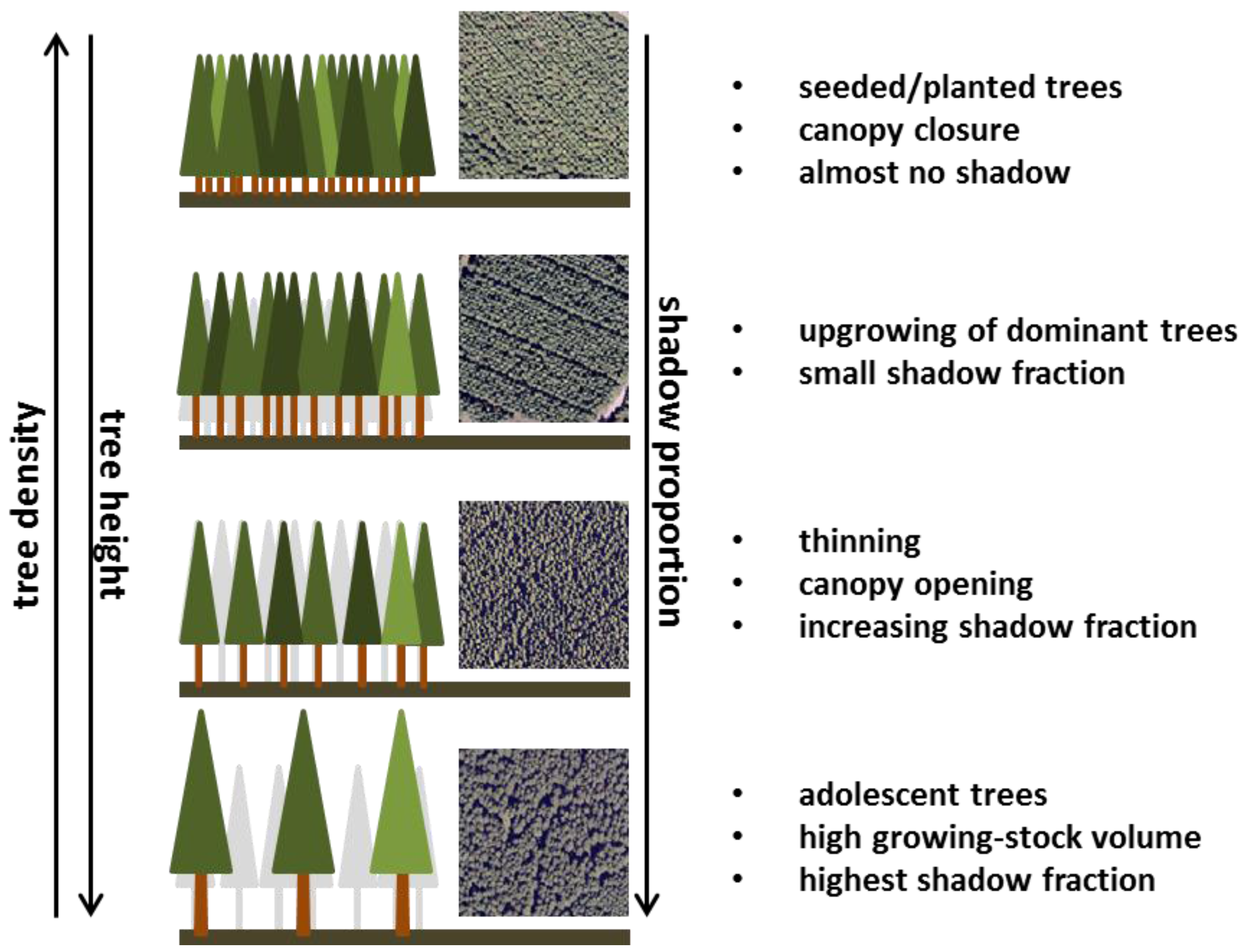
4.1. Sensitive Spectral Ranges
4.2. Estimation Models and Sensors
4.3. Prediction Maps
4.4. Forest Reference Information
5. Conclusions
Acknowledgments
Author Contributions
Appendix


Conflicts of Interest
References
- Foley, J.A.; DeFries, R.; Asner, G.P.; Barford, C.; Bonan, G.; Carpenter, S.R.; Chapin, F.S.; Coe, M.T.; Daily, G.C.; Gibbs, H.K.; et al. Global consequences of land use. Science 2005, 570–574. [Google Scholar] [CrossRef] [PubMed]
- Bond, I.; Grieg-Gran, M.; Wertz-Kanounnikoff, S.; Hazlewood, P.; Wunder, S.; Angelsen, A. Incentives to Sustain Forest Ecosystem Services: A Review and Lessons for REDD; International Institute for Environment and Development: London, UK, 2009. [Google Scholar]
- Food and Agriculture Organization of the United Nations. State of the World’s Forests; FAO: Rome, France, 2012. [Google Scholar]
- Federal Ministry of Food, Agriculture and Consumer Protection. German Forests—Nature and Economic Factor. Available online: http://www.bmel.de/SharedDocs/Downloads/EN/Publications/GermanForests.pdf?_blob=publicationFile (accessed on 13 June 2014).
- Federal Ministry of Food, Agriculture and Consumer Protection. Forest Strategy 2020: Sustainable Forest Management—An Opportunity and a Challenge for Society. Available online: http://www.bmel.de/SharedDocs/Downloads/EN/Publications/ForestStrategy2020.pdf?__blob=publicationFile (accessed on 13 June 2014).
- Bolte, A.; Eisenhauer, D.R.; Erhart, H.P.; Grpß, J.; Hanewinkel, M.; Kölling, C.; Profft, I.; Rohde, M.; Röhe, P.; Amereller, K. Klimawandel und Forstwirtschaft—Übereinstimmungen und Unterschiede bei der Einschätzung der Anpassungsnotwendigkeiten und Anpassungsstrategien der Bundesländer. Landbauforsch. vTI Agric. Forest Res. 2009, 59, 267–278. [Google Scholar]
- Standing Forestry Committee. Ad Hoc Working Group on Forest Information and Monitoring: Final Report. Available online: http://ec.europa.eu/environment/forests/pdf/Fin%20report%20info%20monit%20wg.pdf (accessed on 13 June 2014).
- Peerenboom, H.G.; Ontrup, G.; Böhmer, O. Weiterentwicklung der Forsteinrichtung in Rheinland-Pfalz. Forst und Holz 2003, 58, 728–731. [Google Scholar]
- Köhl, M. New approaches for multi resource forest inventories. In Advances in Forest Inventory for Sustainable Forest Management and Biodiversity Monitoring; Corona, P., Köhl, M., Marchetti, M., Eds.; Springer Netherland: Dordrecht, The Netherlands, 2003. [Google Scholar]
- Potapov, P.V.; Yaroshenko, A.; Turubanova, S.; Dubinin, M.; Laestadius, L.; Thies, C.; Aksenov, D.; Egorov, A.; Yesipova, Y.; Glushkov, I.; et al. Mapping the world’s intact forest landscapes by remote sensing. Available online: https://dlc.dlib.indiana.edu/dlc/bitstream/handle/10535/2817/ES-2008-2670.pdf?sequence=1&isAllowed=y (accessed on 28 July 2015).
- Hansen, M.C.; Stehman, S.V.; Potapov, P.V. Quantification of global gross forest cover loss. Proc. Natl. Acad. Sci. 2010, 107, 8650–8655. [Google Scholar] [CrossRef] [PubMed]
- Hansen, M.C.; Potapov, P.V.; Moore, R.; Hancher, M.; Turubanova, S.A.; Tyukavina, A.; Thau, D.; Stehman, S.V.; Goetz, S.J.; Loveland, T.R.; et al. High-resolution global maps of 21st-century forest cover change. Science 2013, 342, 850–853. [Google Scholar] [CrossRef] [PubMed]
- Food and Agriculture Organisation of the United Nations & European Commission Joint Research Centre. Global Forest Land-Use Change: 1990–2005; FAO & JRC: Rome, France, 2012. [Google Scholar]
- Le Toan, T.; Quegan, S.; Davidson, M.; Balzter, H.; Paillou, P.; Papathanassiou, K.; Plummer, S.; Rocca, F.; Saatchi, S.; Shugart, H.; et al. The BIOMASS mission: Mapping global forest biomass to better understand the terrestrial carbon cycle. Remote Sens. Environ. 2011, 115, 2850–2860. [Google Scholar] [CrossRef]
- Rosenqvist, Å.; Milne, A.; Lucas, R.; Imhoff, M.; Dobson, C. A review of remote sensing technology in support of the Kyoto Protocol. Environ. Sci. Policy 2003, 6, 441–455. [Google Scholar]
- Martin, M.E.; Newman, S.D.; Aber, J.D.; Congalton, R.G. Determining forest species composition using high spectral resolution remote sensing data. Remote Sens. Environ. 1998, 65, 249–254. [Google Scholar] [CrossRef]
- Schlerf, M.; Atzberger, C.; Hill, J. Remote sensing of forest biophysical variables using HyMap imaging spectrometer data. Remote Sens. Environ. 2005, 95, 177–194. [Google Scholar] [CrossRef]
- Stoffels, J.; Mader, S.; Hill, J.; Werner, W.; Ontrup, G. Satellite-based stand-wise forest cover type mapping using a spatially adaptive classification approach. Eur. J. Forest Res. 2012, 131, 1071–1089. [Google Scholar] [CrossRef]
- Franklin, S.E. Remote Sensing for Sustainable Forest Management; CRC Press: Boca Raton, FL, USA, 2001. [Google Scholar]
- Tomppo, E.; Katila, M.; Mäkisara, K.; Peräsaari, J. The multi-source national forest inventory of Finland—Methods and results 2007. Available online: http://www.metla.fi/julkaisut/workingpapers/2012/mwp227.pdf (accessed on 28 July 2015).
- Reese, H.; Nilsson, M.; Granqvist Pahlén, T.; Hagner, O.; Tingelöf, U.; Egberth, M.; Olsson, H. Countrywide estimates of forest variables using satellite data and field data from the National Forest Inventory. AMBIO 2003, 32, 542–548. [Google Scholar] [CrossRef] [PubMed]
- Nilsson, M.; Bohlin, J.; Olsson, H.; Svensson, S.A.; Haapaniemi, M. Operational use of remote sensing for regional level assessment of forest estate values. In New Strategies for European Remote Sensing, Proceedings of the 24th Symposium of the European Association of Remote Sensing Laboratories, Dubrovnik, Croatia, 25–27 May 2004; Oluić, M., Ed.; Mill Press: Dubrovnik, Croatia, 2005; pp. 263–268. [Google Scholar]
- Gjertsen, A. Accuracy of forest mapping based on Landsat TM data and a kNN-based method. Remote Sens. Environ. 2007, 110, 420–430. [Google Scholar] [CrossRef]
- McInerney, D.O.; Nieuwenhuis, M. A comparative analysis of kNN and decision tree methods for the Irish National Forest Inventory. Int. J. Remote Sens. 2009, 30, 4937–4955. [Google Scholar] [CrossRef]
- Koukal, T. Nonparametric Assessment of Forest Attributes by Combination of Field Data of the Austrian Forest Inventory and Remote Sensing Data. Available online: http://citeseerx.ist.psu.edu/viewdoc/download?doi=10.1.1.88.5946&rep=rep1&type=pdf (accessed on 28 July 2015).
- Maselli, F.; Chirici, G.; Bottai, L.; Corona, P.; Marchetti, M. Estimation of Mediterranean forest attributes by the application of k-NN procedures to multitemporal Landsat ETM+ images. Int. J. Remote Sens. 2005, 26, 3781–3796. [Google Scholar] [CrossRef] [Green Version]
- Dees, M.; Duvenhorst, J.; Gross, C.P.; Koch, B. Combining Remote Sensing Data Sources and Terrestrial Sample-based Inventory Data for the Use in Forest Management Inventories. Available online: http://www.isprs.org/proceedings/XXXIII/congress/part7/355_XXXIII-part7.pdf (accessed on 28 July 2015).
- Diemer, C.; Lucaschewsky, I.; Spelsberg, G.; Tomppo, E.; Pekkarinen, A. Integration of terrestrial forest sample plot data, map information and satellite data: An operational multisource inventory concept. In Fusion of Earth Data: Merging Point Measurements, Raster Maps and Remotely Sensed Images; Ranchin, T., Wald, L., Eds.; SEE/URISCA: Nice, France, 2000; pp. 143–150. [Google Scholar]
- Scheuber, M. Potentials and limits of the k-nearest-neighbour method for regionalising sample-based data in forestry. Eur. J. Forest Res. 2009, 129, 825–832. [Google Scholar] [CrossRef]
- Lu, D. The potential and challenge of remote sensing-based biomass estimation. Int. J. Remote Sens. 2006, 27, 1297–1328. [Google Scholar] [CrossRef]
- Gleason, C.J.; Im, J. A review of remote sensing of forest biomass and biofuel: Options for small-area applications. GISci. Remote Sens. 2011, 48, 141–170. [Google Scholar] [CrossRef]
- Koch, B. Status and future of laser scanning, synthetic aperture radar and hyperspectral remote sensing data for forest biomass assessment. ISPRS J. Photogramm. Remote Sens. 2010, 65, 581–590. [Google Scholar] [CrossRef]
- Drusch, M.; Del Bello, U.; Carlier, S.; Colin, O.; Fernandez, V.; Gascon, F.; Hoersch, B.; Isola, C.; Laberinti, P.; Martimort, P. Sentinel-2: ESA’s optical high-resolution mission for GMES operational services. Remote Sens. Environ. 2012, 120, 25–36. [Google Scholar] [CrossRef]
- Malenovský, Z.; Rott, H.; Cihlar, J.; Schaepman, M.E.; García-Santos, G.; Fernandes, R.; Berger, M. Sentinels for science: Potential of Sentinel-1, -2, and -3 missions for scientific observations of ocean, cryosphere, and land. Remote Sens. Environ. 2012, 120, 91–101. [Google Scholar] [CrossRef]
- Kaufmann, H.; Hill, J.; Hostert, P.; Krasemann, H.; Mauser, W.; Müller, A. Science Plan of the Environmental Mapping and Analysis Program (EnMAP). Available online: http://www.enmap.org/ (accessed on 28 July 2015).
- Wolff, B.; Erhard, M.; Holzhausen, M.; Kuhlow, T. Das Klima in den forstlichen Wuchsgebieten und Wuchsbezirken Deutschlands; Wiedebusch: Hamburg, Germany, 2003. [Google Scholar]
- Cocks, T.; Jenssen, R.; Stewart, A.; Wilson, I.; Shields, T. The HyMap TM airborne hyperspectral sensor: The system, calibration and performance. In Proceedings of 1st EARSeL Workshop on Imaging Spectroscopy, EARSeL Paris, France, 6–8 October 1998; pp. 37–42.
- Schläpfer, D.; Schaepman, M.E.; Itten, K. PARGE: parametric geocoding based on GCP-calibrated auxiliary data. Proc. SPIE 1998. [Google Scholar] [CrossRef]
- Schläpfer, D.; Richter, R. Geo-atmospheric processing of airborne imaging spectrometry data: Part 1: parametric orthorectification. Int. J. Remote Sens. 2002, 23, 2609–2630. [Google Scholar]
- Buddenbaum, H.; Schlerf, M.; Hill, J. Classification of coniferous tree species and age classes using hyperspectral data and geostatistical methods. Int. J. Remote Sens. 2005, 26, 5453–5465. [Google Scholar] [CrossRef]
- Hill, J.; Mehl, W.; Radeloff, V. Improved forest mapping by combining corrections of atmospheric and topographic effects in Landsat TM imagery. In Proceedings of the 14th Sensors and environmental applications of remote sensing EARSel Symposium, Goẗeborg, Sweden, 6–8 June 1994.
- Hill, J.; Mehl, W. Geo- und radiometrische Aufbereitung multi- und hyperspektraler Daten zur Erzeugung langjähriger kalibrierter Zeitreihen. Photogrammetrie Fernerkundung Geoinf. 2003, 7, 7–14. [Google Scholar]
- Tanré, D. Description of a computer code to simulate signal in the solar spectrum: The 5S code. Int. J. Remote Sens. 1990. [Google Scholar] [CrossRef]
- Buddenbaum, H.; Seeling, S.; Hill, J. Fusion of full-waveform Lidar and imaging spectroscopy remote sensing data for the characterization of forest stands. Int. J. Remote Sens. 2013, 34, 4511–4524. [Google Scholar] [CrossRef]
- Guanter, L.; Segl, K.; Kaufmann, H. Simulation of optical remote-sensing scenes with application to the EnMAP hyperspectral mission. IEEE Trans. Geosci. Remote Sens. 2009, 47, 2340–2351. [Google Scholar] [CrossRef]
- Martimort, P.; Berger, M.; Carnicero, B.; Del Bello, U.; Fernandez, V.; Gascon, F.; Silvestrin, P.; Spoto, F.; Sy, O.; Arino, O.; et al. Sentinel-2: The optical high-resolution mission for GMES operational services. Eur. Space Agency Bull. 2007, 18–24. [Google Scholar]
- Landesforsten Rheinland-Pfalz. Available online: http://www.wald-rlp.de/ueber-uns/nachhaltigkeit/sicherung-der-nachhaltigkeit/mittelfristigebetriebsplanungforsteinrichtung/inventur.html (accessed on 23 May 2014).
- Trotter, C.M.; Dymond, J.R.; Goulding, C.J. Estimation of timber volume in a coniferous plantation forest using Landsat TM. Int. J. Remote Sens. 1997, 18, 2209–2223. [Google Scholar] [CrossRef]
- Reese, H.; Nilsson, M.; Sandström, P.; Olsson, H. Applications using estimates of forest parameters derived from satellite and forest inventory data. Comput. Electron. Agr. 2002, 37, 37–55. [Google Scholar] [CrossRef]
- Thünen Institut. Dritte Bundeswaldinventur-Ergebnisdatenbank, Auftragskürzel 77Z1PB_L458mf_0212_biHb, Archivierungsdatum: 2014–12–22 20:2:36.107, Überschrift: Zuwachs des Vorrates [m³/ha*a] nach Land und Baumartengruppe (rechnerischer Reinbestand), Filter: Periode=2002–2012. Available online: https://bwi.info (accessed on 30 June 2015).
- Wold, S.; Sjöström, M.; Eriksson, L. PLS-regression: A basic tool of chemometrics. Chemometr. Intell. Lab. 2001, 58, 109–130. [Google Scholar] [CrossRef]
- Farifteh, J.; van der Meer, F.; Atzberger, C.; Carranza, E. Quantitative analysis of salt-affected soil reflectance spectra: A comparison of two adaptive methods (PLSR and ANN). Remote Sens. Environ. 2007, 110, 59–78. [Google Scholar] [CrossRef]
- Asner, G.; Martin, R. Spectral and chemical analysis of tropical forests: Scaling from leaf to canopy levels. Remote Sens. Environ. 2008, 112, 3958–3970. [Google Scholar] [CrossRef]
- Zhang, J.; Wu, J.; Zhou, L. Deriving vegetation leaf water content from spectrophotometric data with orthogonal signal correction-partial least square regression. Int. J. Remote Sens. 2011, 32, 7557–7574. [Google Scholar] [CrossRef]
- Axelsson, C.; Skidmore, A.K.; Schlerf, M.; Fauzi, A.; Verhoef, W. Hyperspectral analysis of mangrove foliar chemistry using PLSR and support vector regression. Int. J. Remote Sens. 2013, 34, 1724–1743. [Google Scholar] [CrossRef]
- Wolter, P.T.; Townsend, P.A.; Sturtevant, B.R. Estimation of forest structural parameters using 5 and 10 meter SPOT-5 satellite data. Remote Sens. Environ. 2009, 113, 2019–2036. [Google Scholar] [CrossRef]
- Lei, C.; Ju, C.Y.; Cai, T.J.; Jing, X.; Wei, X.H.; Di, X.Y. Estimating canopy closure density and above-ground tree biomass using partial least square methods in Chinese boreal forests. J. Forest Res. 2012, 23, 191–196. [Google Scholar] [CrossRef]
- Vaglio Laurin, G.; Chen, Q.; Lindsell, J.A.; Coomes, D.A.; Frate, F.D.; Guerriero, L.; Pirotti, F.; Valentini, R. Above ground biomass estimation in an African tropical forest with Lidar and hyperspectral data. ISPRS J. Photogramm. Remote Sens. 2014, 89, 49–58. [Google Scholar] [CrossRef]
- Tomppo, E.; Olsson, H.; Ståhl, G.; Nilsson, M.; Hagner, O.; Katila, M. Combining national forest inventory field plots and remote sensing data for forest databases. Remote Sens. Environ. 2008, 112, 1982–1999. [Google Scholar] [CrossRef]
- Gong, G. Crossvalidation, The Jackknife, and the Bootstrap: Excess Error Estimation in Forward Logistic Regression. Ph.D. Thesis, Stanford University, Stanford, CA, USA, 1982. [Google Scholar]
- Höskuldsson, A. PLS regression methods. J. Chemometr. 1988, 2, 211–228. [Google Scholar] [CrossRef]
- Buddenbaum, H.; Steffens, M. Mapping the distribution of chemical properties in soil profiles using laboratory imaging spectroscopy, SVM and PLS regression. EARSeL eProc. 2012, 11, 25–32. [Google Scholar]
- Katila, M.; Tomppo, E. Selecting estimation parameters for the Finnish multisource National Forest Inventory. Remote Sens. Environ. 2001, 76, 16–32. [Google Scholar] [CrossRef]
- Kilpeläinen, P.; Tokola, T. TM image-based estimates of stand volume. Forest Ecol. Manag. 1999, 124, 105–111. [Google Scholar] [CrossRef]
- Heiskanen, J. Estimating aboveground tree biomass and leaf area index in a mountain birch forest using ASTER satellite data. Int. J. Remote Sens. 2006, 27, 1135–1158. [Google Scholar] [CrossRef]
- Ardö, J. Volume quantification of coniferous forest compartments using spectral radiance recorded by Landsat Thematic Mapper. Int. J. Remote Sens. 1992, 13, 1779–1786. [Google Scholar] [CrossRef]
- Gemmell, F. Effects of forest cover, terrain and scale on timber volume estimation with TM data in a Rocky Mountain site. Remote Sens. Environ. 1995, 51, 294–305. [Google Scholar] [CrossRef]
- Muukkonen, P.; Heiskanen, J. Estimating biomass for boreal forests using ASTER satellite data combined with standwise forest inventory data. Remote Sens. Environ. 2005, 99, 434–447. [Google Scholar] [CrossRef]
- Stenberg, P. Penumbra in within-shoot and between-shoot shading in conifers and its significance for photosynthesis. Ecol. Model. 1995, 77, 215–231. [Google Scholar] [CrossRef]
- Smolander, S.; Stenberg, P. A method to account for shoot scale clumping in coniferous canopy reflectance models. Remote Sens. Environ. 2003, 88, 363–373. [Google Scholar] [CrossRef]
- Vohland, M.; Stoffels, J.; Hau, C.; Schüler, G. Remote sensing techniques for forest parameter assessment: Multispectral classification and linear spectral mixture analysis. Silva Fennica 2007, 41, 441–456. [Google Scholar] [CrossRef]
- Hawkins, D.M. The problem of overfitting. J. Chem. Inf. Model. 2004, 44, 1–12. [Google Scholar] [CrossRef] [PubMed]
- Atzberger, C.; Guérif, M.; Baret, F.; Werner, W. Comparative analysis of three chemometric techniques for the spectroradiometric assessment of canopy chlorophyll content in winter wheat. Comput. Electron. Agr. 2010, 73, 165–173. [Google Scholar] [CrossRef]
- Raykov, T.; Marcoulides, G.A. An Introduction to Applied Multivariate analysis; Routledge: New York, NY, USA, 2008. [Google Scholar]
- Hyyppä, J.; Hyyppä, H.; Inkinen, M.; Engdahl, M.; Linko, S.; Zhu, Y.-H. Accuracy comparison of various remote sensing data sources in the retrieval of forest stand attributes. Forest Ecol. Manag. 2000, 128, 109–120. [Google Scholar] [CrossRef]
- McRoberts, R.; Tomppo, E. Remote sensing support for national forest inventories. Remote Sens. Environ. 2007, 110, 412–419. [Google Scholar] [CrossRef]
- Bedison, J.E.; McNeil, B.E. Is the growth of temperate forest trees enhanced along an ambient nitrogen deposition gradient? Ecology 2009, 90, 1736–1742. [Google Scholar] [CrossRef] [PubMed]
- McMahon, S.M.; Parker, G.G.; Miller, D.R. Evidence for a recent increase in forest growth. Proc. Nation. Acad. Sci. 2010, 107, 3611–3615. [Google Scholar] [CrossRef] [PubMed]
- Lausch, A.; Heurich, M.; Gordalla, D.; Dobner, H.J.; Gwillym-Margianto, S.; Salbach, C. Forecasting potential bark beetle outbreaks based on spruce forest vitality using hyperspectral remote-sensing techniques at different scales. Forest Ecol. Manag. 2013, 308, 76–89. [Google Scholar] [CrossRef]
- Jönsson, A.; Appelberg, G.; Harding, S.; Bärring, L. Spatio-temporal impact of climate change on the activity and voltinism of the spruce bark beetle, lps typographus. Glob. Change Biol. 2009, 15, 486–499. [Google Scholar] [CrossRef]
- Marini, L.; Ayres, M.P.; Battisti, A.; Faccoli, M. Climate affects severity and altitudinal distribution of outbreaks in an eruptive bark beetle. Clim. Change 2012, 115, 327–341. [Google Scholar] [CrossRef]
© 2015 by the authors; licensee MDPI, Basel, Switzerland. This article is an open access article distributed under the terms and conditions of the Creative Commons Attribution license (http://creativecommons.org/licenses/by/4.0/).
Share and Cite
Nink, S.; Hill, J.; Buddenbaum, H.; Stoffels, J.; Sachtleber, T.; Langshausen, J. Assessing the Suitability of Future Multi- and Hyperspectral Satellite Systems for Mapping the Spatial Distribution of Norway Spruce Timber Volume. Remote Sens. 2015, 7, 12009-12040. https://doi.org/10.3390/rs70912009
Nink S, Hill J, Buddenbaum H, Stoffels J, Sachtleber T, Langshausen J. Assessing the Suitability of Future Multi- and Hyperspectral Satellite Systems for Mapping the Spatial Distribution of Norway Spruce Timber Volume. Remote Sensing. 2015; 7(9):12009-12040. https://doi.org/10.3390/rs70912009
Chicago/Turabian StyleNink, Sascha, Joachim Hill, Henning Buddenbaum, Johannes Stoffels, Thomas Sachtleber, and Joachim Langshausen. 2015. "Assessing the Suitability of Future Multi- and Hyperspectral Satellite Systems for Mapping the Spatial Distribution of Norway Spruce Timber Volume" Remote Sensing 7, no. 9: 12009-12040. https://doi.org/10.3390/rs70912009