
The Use of Multi-Temporal Landsat Imageries in Detecting Seasonal Crop Abandonment


Abstract
:
1. Introduction
- What is the total area of abandoned paddy and rubber in the study area?
- How accurately can abandoned paddy and rubber areas be identified using rule-based classification with multi-temporal Landsat imageries?
2. Methods
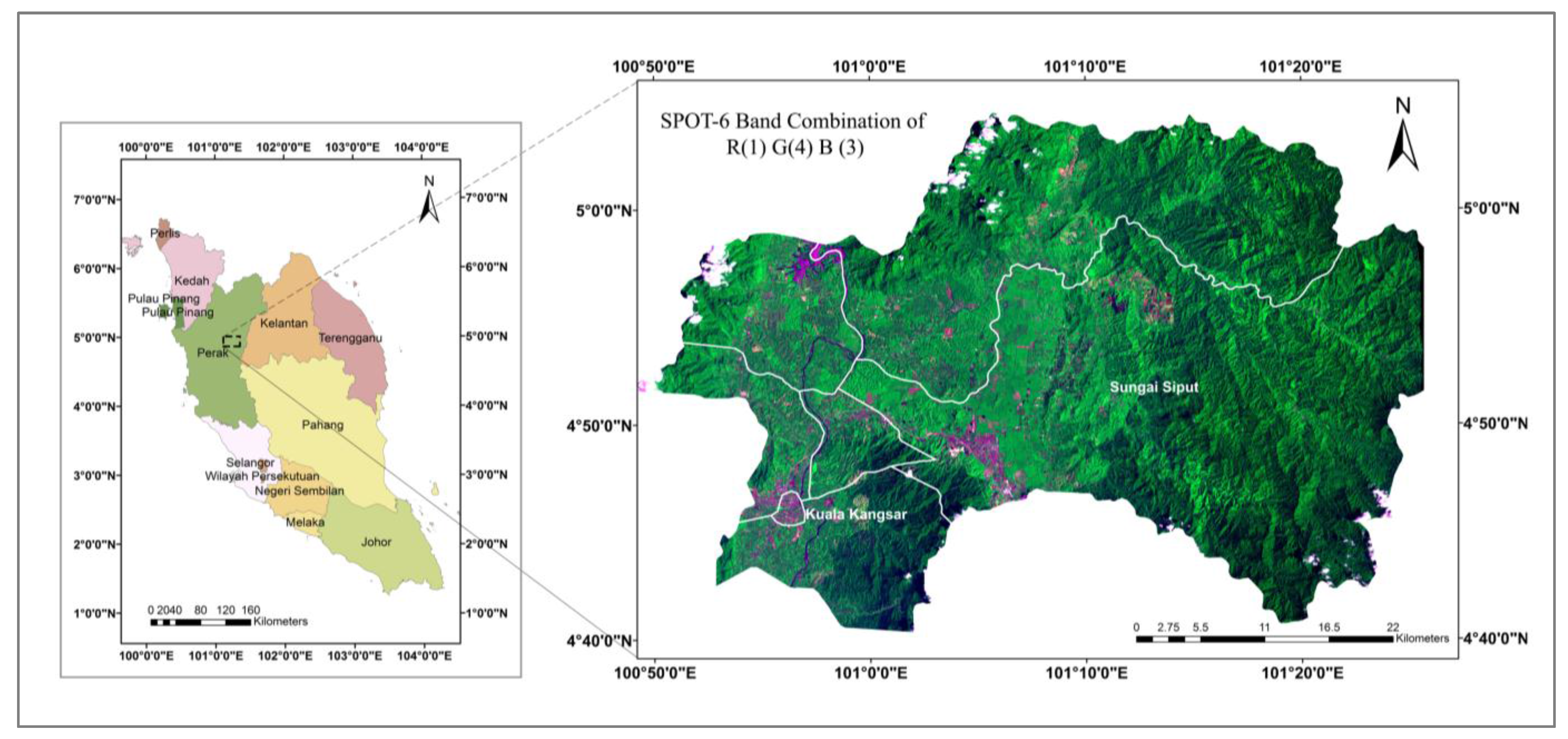
2.1. Study Area
2.2. Data Collection

| Image Date | Sensor | Image Purpose |
|---|---|---|
| 28 May 1997 | TM | Reference for image normalization |
| 21 January 2009 | TM | Supporting the feature extraction of abandoned land |
| 22 April 2013 | OLI | Crop phenology development |
| 9 June 2013 | OLI | Crop phenology development |
| 18 December 2013 | OLI | Crop phenology development |
| 4 February 2014 | OLI | Crop phenology development and classification |
| 24 March 2014 | OLI | Crop phenology development |
| 9 April 2014 | OLI | Crop phenology development |
| 11 May 2014 | OLI | Crop phenology development |
| 28 June 2014 | OLI | Crop phenology development and classification |
| 16 September 2014 | OLI | Crop phenology development and classification |
| 7 February 2015 | OLI | Crop phenology development |
| 23 February 2015 | OLI | Crop phenology development |
| 11 March 2015 | OLI | Crop phenology development |
| 12 April 2015 | OLI | Crop phenology development |
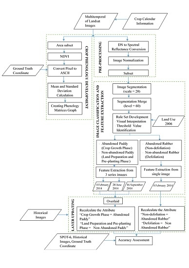
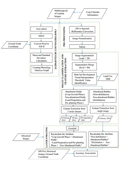
2.3. Crop Phenology Development
2.4. Pre-Processing of Satellite Images
2.4.1. Digital Number (DN) to Reflectance Conversion
2.4.2. Image Normalization
2.5. Image Classification and Feature Extraction
| Paddy | Rubber | |
|---|---|---|
| Primary Image Input | 4 February 2014 28 June 2014 16 September 2014 | 4 February 2014 |
| Ancillary Data Input | NDVI Land use 2006 (Rasterized) | Land use 2006 (Rasterized) |
| Scale Parameter | 20 | 20 |
| Merge Level | 60 | 60 |
| Rule Set | Land preparation phase Land use (Confidence image value) < 210 NDVI < 0.3521 SWIR 1 (Reflectance) > 0.1746 | Non-abandoned Land use (Confidence image value) < 250 NIR (Reflectance) < 0.4760 |
| Pre-Planting (Irrigation phase) Land use (Confidence image value) < 210 NDVI < 0.3521 SWIR 1 (Reflectance) NOT > 0.1746 SWIR 2 (Reflectance) < 0.0544 | Abandoned Land use (Confidence image value) < 250 NIR (Reflectance) NOT < 0.4760 | |
| Crop growth phase Land use (Confidence image value) < 210 SWIR 1 (Reflectance) NOT > 0.1746 SWIR 2 (Reflectance) NOT < 0.0544 |
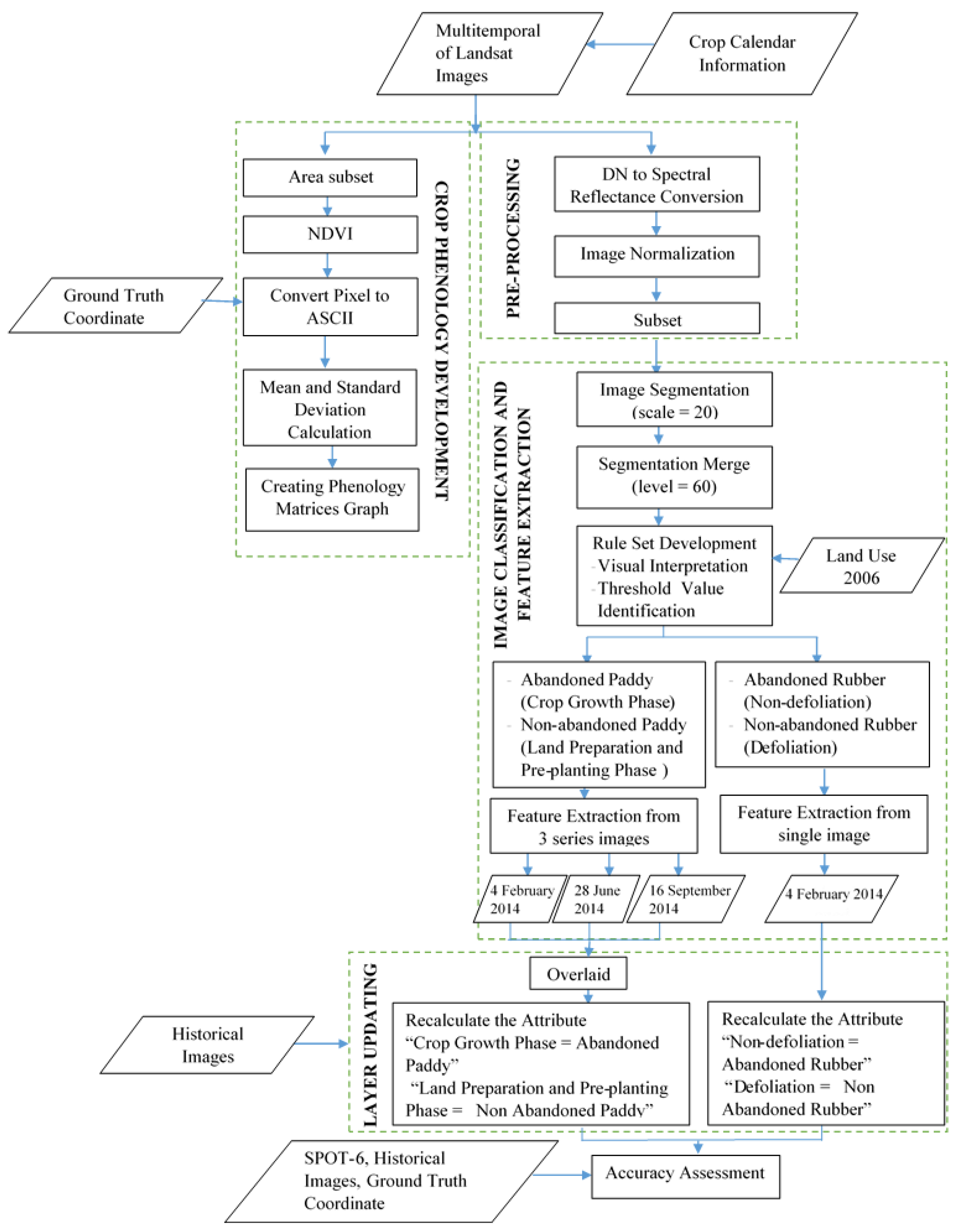
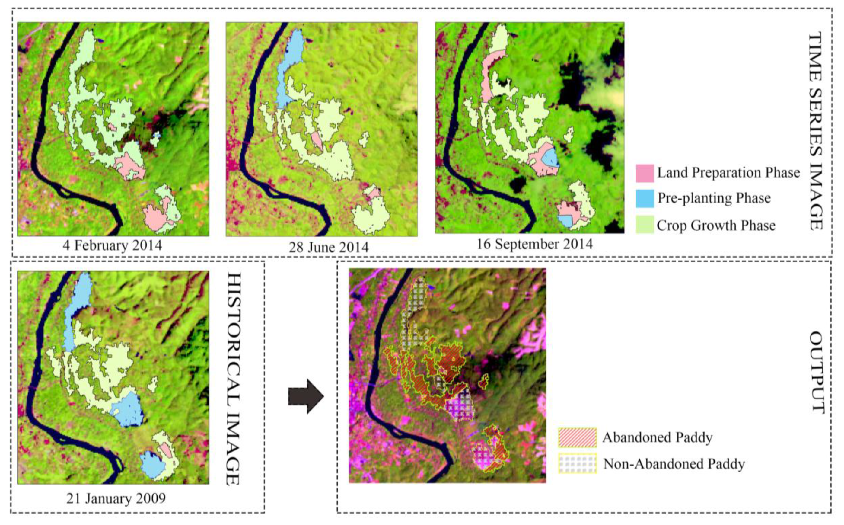
2.6. Layer Updating
2.7. Accuracy Assessment
3. Results and Discussion
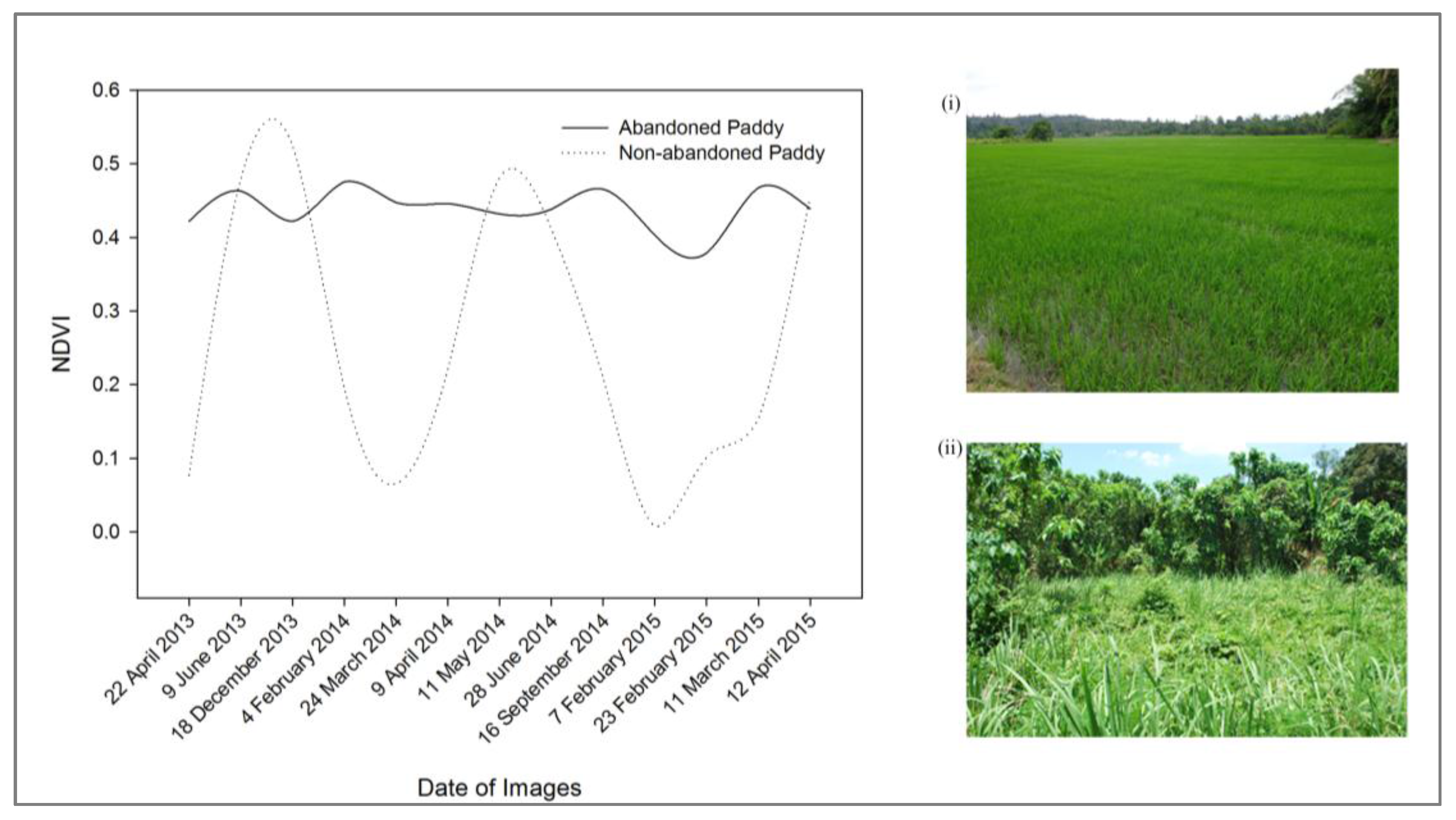
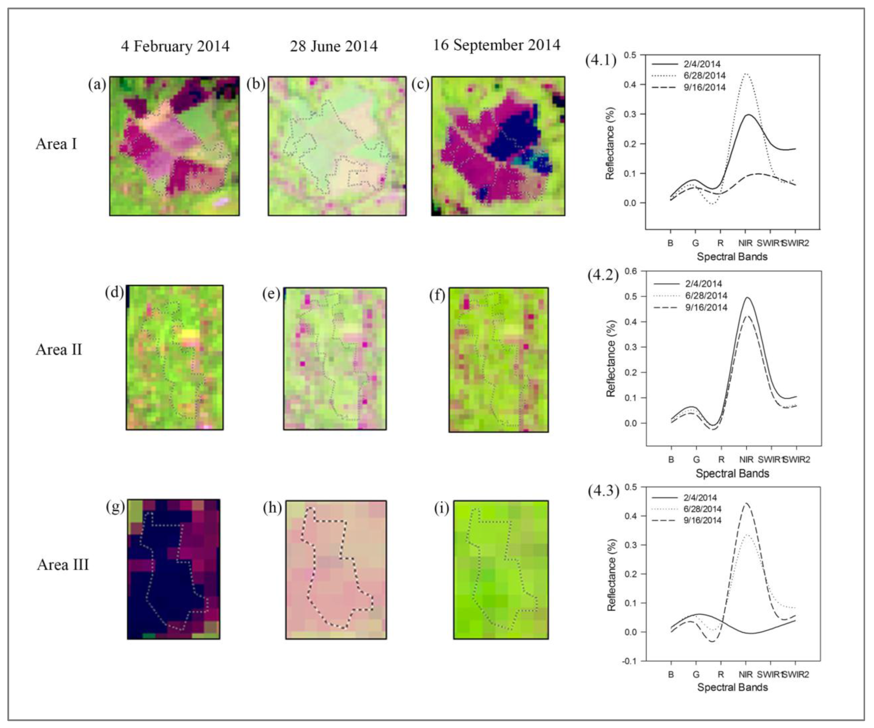
3.1. Crop Phenology
3.1.1. Paddy


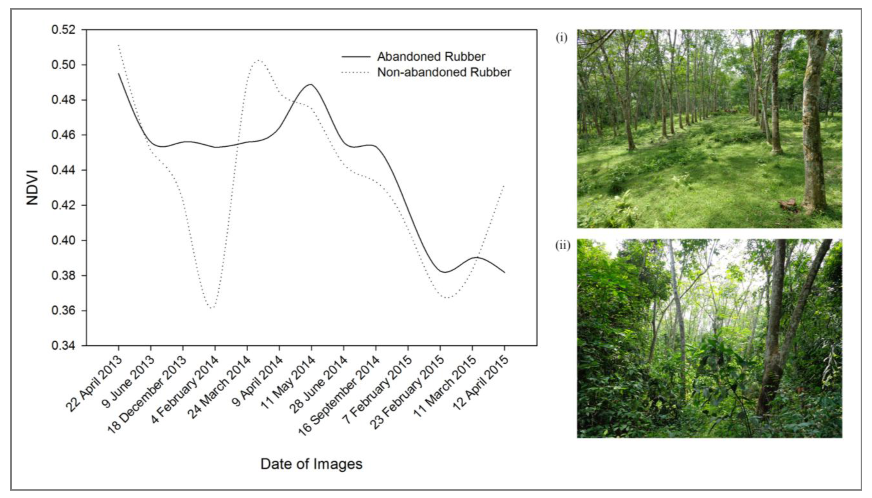
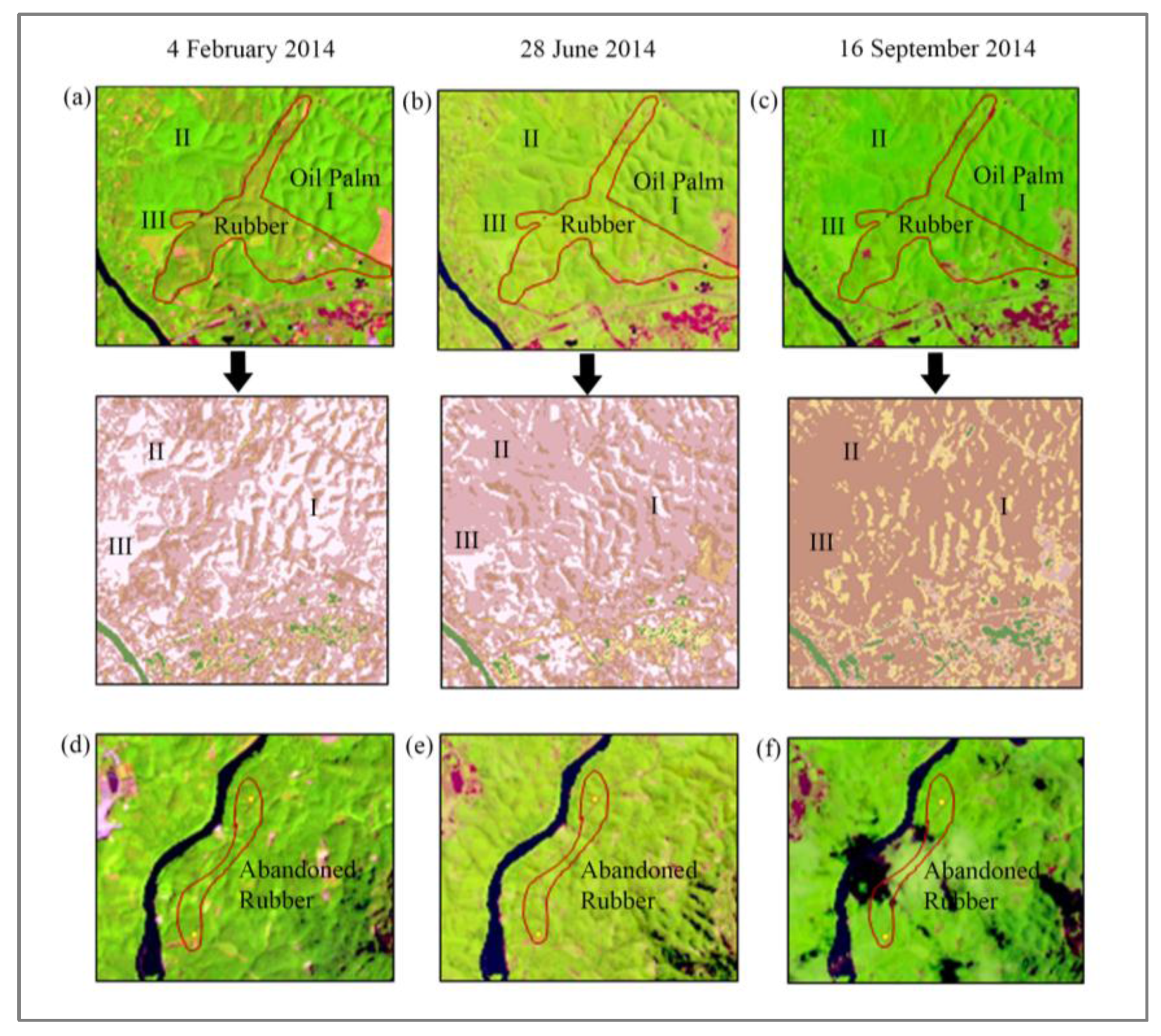
3.1.2. Rubber

3.2. Image Classification and Accuracy Assessment
3.2.1. Paddy

| Abandoned Paddy | Non-abandoned Paddy | Abandoned Rubber | Non-abandoned Rubber | Others | Classification Overall | Producer Accuracy | |
|---|---|---|---|---|---|---|---|
| Abandoned Paddy | 28 | 1 | 0 | 0 | 0 | 29 | 96.55% |
| Non-Abandoned Paddy | 0 | 29 | 0 | 0 | 0 | 29 | 100.00% |
| Abandoned Rubber | 0 | 0 | 25 | 0 | 0 | 25 | 100.00% |
| Non-Abandoned Rubber | 0 | 0 | 5 | 26 | 0 | 31 | 83.87% |
| Others | 2 | 4 | 0 | 6 | 0.00% | ||
| Truth Overall | 30 | 30 | 30 | 30 | 0 | 120 | |
| User Accuracy | 93.33% | 96.67% | 83.33% | 86.67% | No Data |
| Class | Map Area (ha) | Wi | S(p̂) | S(Â) |
|---|---|---|---|---|
| Abandoned Paddy | 579 | 0.006 | 0.1408 | 81.54 |
| Non-Abandoned Paddy | 534 | 0.006 | 0.0002 | 0.12 |
| Abandoned Rubber | 13,068 | 0.135 | 0.0124 | 162.34 |
| Non-Abandoned Rubber | 17,932 | 0.185 | 0.1414 | 2535.11 |
| Others | 64,703 | 0.668 | ||
| Total | 96,816 | 1 |
3.2.2. Rubber
4. Conclusions
Acknowledgments
Author Contributions
Conflicts of Interest
References
- Prishchepov, A.V.; Radeloff, V.C.; Dubinin, M.; Alcantara, C. The effect of Landsat ETM/ETM+ image acquisition dates on the detection of agricultural land abandonment in eastern Europe. Remote Sens. Environ. 2012, 126, 195–209. [Google Scholar] [CrossRef]
- Díaz, G.I.; Nahuelhual, L.; Echeverría, C.; Marín, S. Drivers of land abandonment in southern Chile and implications for landscape planning. Landsc. Urban Plan. 2011, 99, 207–217. [Google Scholar] [CrossRef]
- Koulouri, M.; Giourga, C. Land abandonment and slope gradient as key factors of soil erosion in mediterranean terraced lands. Catena 2007, 69, 274–281. [Google Scholar] [CrossRef]
- Alcantara, C.; Kuemmerle, T.; Baumann, M.; Bragina, E.V.; Griffiths, P.; Hostert, P.; Knorn, J.; Müller, D.; Prishchepov, A.V.; Schierhorn, F.; et al. Mapping the extent of abandoned farmland in central and eastern Europe using MODIS time series satellite data. Environ. Res. Lett. 2013, 8, 035035. [Google Scholar] [CrossRef]
- Munroe, D.K.; van Berkel, D.B.; Verburg, P.H.; Olson, J.L. Alternative trajectories of land abandonment: Causes, consequences and research challenges. Curr. Opin. Environ. Sustain. 2013, 5, 471–476. [Google Scholar] [CrossRef]
- Baumann, M.; Kuemmerle, T.; Elbakidze, M.; Ozdogan, M.; Radeloff, V.C.; Keuler, N.S.; Prishchepov, A.V.; Kruhlov, I.; Hostert, P. Patterns and drivers of post-socialist farmland abandonment in western Ukraine. Land Use Policy 2011, 28, 552–562. [Google Scholar] [CrossRef]
- Milenov, P.; Vassilev, V.; Vassileva, A.; Radkov, R.; Samoungi, V.; Dimitrov, Z.; Vichev, N. Monitoring of the risk of farmland abandonment as an efficient tool to assess the environmental and socio-economic impact of the common agriculture policy. Int. J. Appl. Earth Obs. Geoinf. 2014, 32, 218–227. [Google Scholar] [CrossRef]
- Gellrich, M.; Baur, P.; Koch, B.; Zimmermann, N.E. Agricultural land abandonment and natural forest re-growth in the Swiss mountains: A spatially explicit economic analysis. Agric. Ecosyst. Environ. 2007, 118, 93–108. [Google Scholar] [CrossRef]
- Soukup, T.; Brodsky, L.; Vobora, V. Remote sensing identification and monitoring of abandoned land. Available online: http://www.e-envi2009.org/presentations/S4/Soukup.pdf (accessed on 9 September 2014).
- Department of Agriculture Official Portal. Available online: http://www.doa.gov.my/maklumat-tanah-terbiar (accessed on 12 January 2014).
- Ponnusamy, R. Director, Research and Development Division, Felcra Berhad, Kuala Lumpur, Malaysia; Felcra Plantation Services Sdn.Bhd.: Kuala Lumpur, Malaysia, 2013. [Google Scholar]
- Sikor, T.; Müller, D.; Stahl, J. Land fragmentation and cropland abandonment in Albania: Implications for the roles of state and community in post-socialist land consolidation. World Dev. 2009, 37, 1411–1423. [Google Scholar] [CrossRef]
- Oetter, D.R.; Cohen, W.B.; Berterretche, M.; Maiersperger, T.K.; Kennedy, R.E. Land cover mapping in an agricultural setting using multiseasonal thematic mapper data. Remote Sens. Environ. 2000, 76, 139–155. [Google Scholar] [CrossRef]
- Vieira, M.A.; Formaggio, A.R.; Rennó, C.D.; Atzberger, C.; Aguiar, D.A.; Mello, M.P. Object based image analysis and data mining applied to a remotely sensed Landsat time-series to map sugarcane over large areas. Remote Sens. Environ. 2012, 123, 553–562. [Google Scholar] [CrossRef]
- Atkinson, P.M.; Jeganathan, C.; Dash, J.; Atzberger, C. Inter-comparison of four models for smoothing satellite sensor time-series data to estimate vegetation phenology. Remote Sens. Environ. 2012, 123, 400–417. [Google Scholar] [CrossRef]
- Dong, J.; Xiao, X.; Chen, B.; Torbick, N.; Jin, C.; Zhang, G.; Biradar, C. Mapping deciduous rubber plantations through integration of PALSAR and multi-temporal Landsat imagery. Remote Sens. Environ. 2013, 134, 392–402. [Google Scholar] [CrossRef]
- Dong, J.; Xiao, X.; Sheldon, S.; Biradar, C.; Xie, G. Mapping tropical forests and rubber plantations in complex landscapes by integrating PALSAR and MODIS imagery. ISPRS J. Photogramm. Remote Sens. 2012, 74, 20–33. [Google Scholar] [CrossRef]
- Dong, J.; Xiao, X.; Kou, W.; Qin, Y.; Zhang, G.; Li, L.; Jin, C.; Zhou, Y.; Wang, J.; Biradar, C.; et al. Tracking the dynamics of paddy rice planting area in 1986–2010 through time series Landsat images and phenology-based algorithms. Remote Sens. Environ. 2015, 160, 99–113. [Google Scholar] [CrossRef]
- Stefanski, J.; Chaskovskyy, O.; Waske, B. Mapping and monitoring of land use changes in post-soviet western ukraine using remote sensing data. Appl. Geogr. 2014, 55, 155–164. [Google Scholar] [CrossRef]
- Hussain, M.; Chen, D.; Cheng, A.; Wei, H.; Stanley, D. Change detection from remotely sensed images: From pixel-based to object-based approaches. ISPRS J. Photogramm. Remote Sens. 2013, 80, 91–106. [Google Scholar] [CrossRef]
- Wang, Z.; Jensen, J.R.; Im, J. An automatic region-based image segmentation algorithm for remote sensing applications. Environ. Model. Softw. 2010, 25, 1149–1165. [Google Scholar] [CrossRef]
- Gamanya, R.; de Maeyer, P.; de Dapper, M. Object-oriented change detection for the city of Harare, Zimbabwe. Expert Syst. Appl. 2009, 36, 571–588. [Google Scholar] [CrossRef]
- Hall, O.; Hay, G.J. A multiscale object-specific approach to digital change detection. Int. J. Appl. Earth Obs. Geoinf. 2003, 4, 311–327. [Google Scholar] [CrossRef]
- Stumpf, A.; Kerle, N. Object-oriented mapping of landslides using random forests. Remote Sens. Environ. 2011, 115, 2564–2577. [Google Scholar] [CrossRef]
- Mallinis, G.; Koutsias, N.; Tsakiri-Strati, M.; Karteris, M. Object-based classification using quickbird imagery for delineating forest vegetation polygons in a Mediterranean test site. ISPRS J. Photogramm. Remote Sens. 2008, 63, 237–250. [Google Scholar] [CrossRef]
- Abu Bakar, H.A. Teknologi Perladangan dan Pemprosesan Getah; Malaysian Rubber Board: Sungai Buloh, Malaysia, 2009. [Google Scholar]
- Muhamad Hafiz, A.R. Geospatial Manager; Felcra Plantation Services Sdn.Bhd.: Kuala Lumpur, Malaysia, 2014. [Google Scholar]
- Guyot, F.B.A.G. Potentials and limits of vegetation indices for LAI and APAR assessment. Remote Sens. Environ. 1991, 35, 161–173. [Google Scholar]
- Leclerc, G.; Hall, C.A.S. Remote Sensing and Land Use Analysis for Agriculture in Costa Rica; Academic Press: New York, NJ, USA, 2000. [Google Scholar]
- Atzberger, C.; Klisch, A.; Mattiuzzi, M.; Vuolo, F. Phenological metrics derived over the european continent from NDVI3g data and MODIS time series. Remote Sens. 2013, 6, 257–284. [Google Scholar] [CrossRef]
- Li, Z.; Fox, J.M. Mapping rubber tree growth in mainland southeast Asia using time-series MODIS 250 m NDVI and statistical data. Appl. Geogr. 2012, 32, 420–432. [Google Scholar] [CrossRef]
- De Bie, C.A.J.M.; Khan, M.R.; Smakhtin, V.U.; Venus, V.; Weir, M.J.C.; Smaling, E.M.A. Analysis of multi-temporal SPOT NDVI images for small-scale land-use mapping. Int. J. Remote Sens. 2011, 32, 6673–6693. [Google Scholar] [CrossRef]
- USGS. Using the USGS Landsat 8 Product. Available online: http://Landsat.usgs.gov (accessed on 20 January 2015).
- Chander, G.; Markham, B.L.; Helder, D.L. Summary of current radiometric calibration coefficients for Landsat MSS, TM, ETM+, and EO-1 ALI sensors. Remote Sens. Environ. 2009, 113, 893–903. [Google Scholar] [CrossRef]
- Vicenteserrano, S.; Perezcabello, F.; Lasanta, T. Assessment of radiometric correction techniques in analyzing vegetation variability and change using time series of Landsat images. Remote Sens. Environ. 2008, 112, 3916–3934. [Google Scholar] [CrossRef]
- Pratt, W.K. Digital Image Processing; John Wiley & Sons, Inc.: New York, NJ, USA, 1991. [Google Scholar]
- ESRI. Band Combinations for Landsat 8. Available online: http://blogs.esri.com/esri/arcgis/2013/07/24/band-combinations-for-Landsat-8/ (accessed on 20 January 2015).
- Lian, L.; Chen, J. Research on segmentation scale of multi-resources remote sensing data based on object-oriented. Procedia Earth Planet. Sci. 2011, 2, 352–357. [Google Scholar] [CrossRef]
- Gamanya, R.; de Maeyer, P.; de Dapper, M. An automated satellite image classification design using object-oriented segmentation algorithms: A move towards standardization. Expert Syst. Appl. 2007, 32, 616–624. [Google Scholar] [CrossRef]
- Karydas, C.G.; Gitas, I.Z. Development of an IKONOS image classification rule-set for multi-scale mapping of mediterranean rural landscapes. Int. J. Remote Sens. 2011, 32, 9261–9277. [Google Scholar] [CrossRef]
- Congalton, R.G. A review of assessing the accuracy of classifications of remotely sensed data. Remote Sens. Environ. 1991, 37, 35–46. [Google Scholar] [CrossRef]
- Olofsson, P.; Foody, G.M.; Stehman, S.V.; Woodcock, C.E. Making better use of accuracy data in land change studies: Estimating accuracy and area and quantifying uncertainty using stratified estimation. Remote Sens. Environ. 2013, 129, 122–131. [Google Scholar] [CrossRef]
- Department, M.M. Monthly Weather Bulletin. Available online: http://www.met.gov.my/ (accessed on 29 May 2015).
© 2015 by the authors; licensee MDPI, Basel, Switzerland. This article is an open access article distributed under the terms and conditions of the Creative Commons Attribution license (http://creativecommons.org/licenses/by/4.0/).
Share and Cite
Yusoff, N.M.; Muharam, F.M. The Use of Multi-Temporal Landsat Imageries in Detecting Seasonal Crop Abandonment. Remote Sens. 2015, 7, 11974-11991. https://doi.org/10.3390/rs70911974
Yusoff NM, Muharam FM. The Use of Multi-Temporal Landsat Imageries in Detecting Seasonal Crop Abandonment. Remote Sensing. 2015; 7(9):11974-11991. https://doi.org/10.3390/rs70911974
Chicago/Turabian StyleYusoff, Noryusdiana Mohamad, and Farrah Melissa Muharam. 2015. "The Use of Multi-Temporal Landsat Imageries in Detecting Seasonal Crop Abandonment" Remote Sensing 7, no. 9: 11974-11991. https://doi.org/10.3390/rs70911974
APA StyleYusoff, N. M., & Muharam, F. M. (2015). The Use of Multi-Temporal Landsat Imageries in Detecting Seasonal Crop Abandonment. Remote Sensing, 7(9), 11974-11991. https://doi.org/10.3390/rs70911974