
Large Scale Automatic Analysis and Classification of Roof Surfaces for the Installation of Solar Panels Using a Multi-Sensor Aerial Platform


Abstract
:
1. Introduction
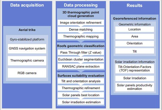
2. Materials and Methods
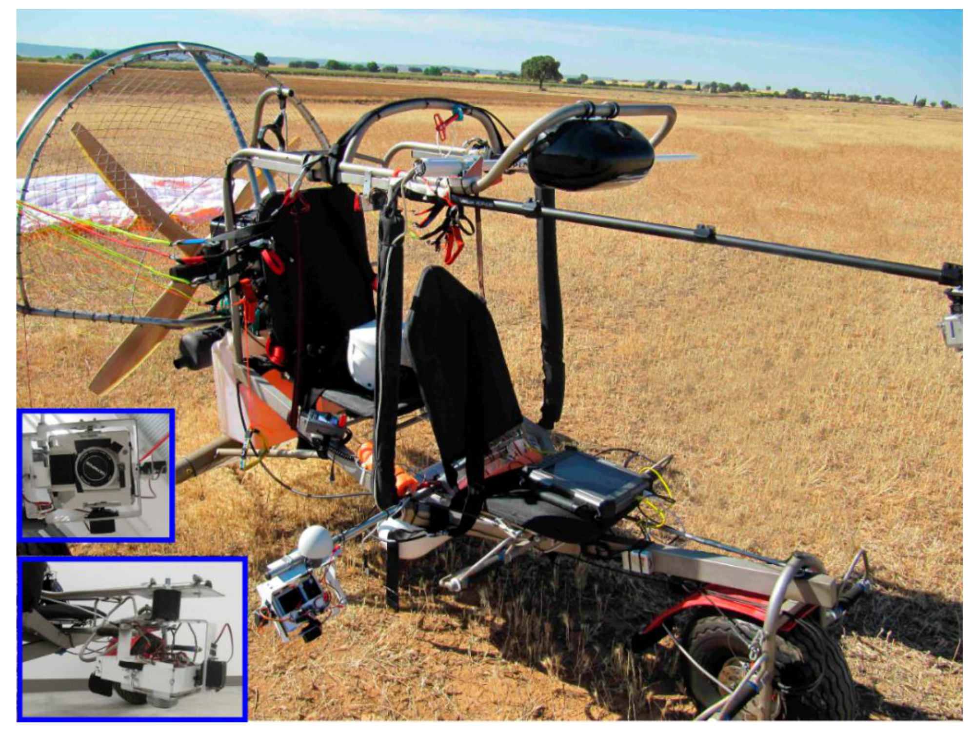
2.1. Equipment
2.1.1. Aerial Trike

| Parameter | Value |
|---|---|
| Empty weight | 110 kg |
| Maximum load | 220 kg |
| Autonomy | 3.5 h |
| Maximum speed | 60 km/h |
| Motor | Rotax 503 |
| Tandem paraglide | MACPARA Pasha 4 |
| Emergency system | Ballistic parachutes GRS 350 |
| Gimbal | Stabilized with 2 degrees of freedom (MUSAS) |
| Minimum sink rate | 1.10 |
| Maximum glide rate | 8.60 |
| Plant surface | 42.23 m2 |
| Projected area | 37.80 m2 |
| Wingspan | 15.03 m |
| Plant elongation rate | 5.35 |
| Central string | 3.51 m |
| Boxes | 54 boxes |
| Zoom factor | 100% |

2.1.2. RGB Camera
| Parameter | -- | Value |
|---|---|---|
| Focal length (mm) | Value | 50.1 |
| Format size (mm) | Value | 34.819 × 23.213 |
| Principal point displacement (mm) | X value | −0.21 |
| Y value | −0.11 | |
| Radial lens distortion | K1 value (mm−2) | 6.035546 × 10⁻⁵ |
| K2 value (mm−4) | −1.266639 × 10⁻⁸ | |
| Decentering lens distortion | P1 value (mm−1) | 1.585075 × 10⁻⁵ |
| P2 value (mm−1) | 6.541129 × 10⁻⁵ | |
| Point marking residuals | Overall RMSE (pixels) | 0.244 |
2.1.3. Thermographic Camera

| Parameter | -- | Value | Std. Deviation |
|---|---|---|---|
| Focal length (mm) | Value | 25.063 | 0.022 |
| Format size (mm) | Value | 10.874 × 8.160 | 0.002 |
| Principal point displacement (mm) | X value | −0.174 | 0.022 |
| Y value | 0.024 | 0.026 | |
| Radial lens distortion | K1 value (mm−2) | 5.281 × 10⁻⁵ | 2.4 × 10⁻⁵ |
| K2 value (mm−4) | 7.798 × 10⁻⁷ | 6.1 × 10⁻⁷ | |
| Decentering lens distortion | P1 value (mm−1) | 1.023 × 10⁻⁴ | 1.2 × 10⁻⁵ |
| P2 value (mm−1) | −3.401 × 10⁻⁵ | 1.3 × 10⁻⁵ | |
| Point marking residuals (pixels) | Overall RMSE | 0.173 | -- |
2.2. Methodology
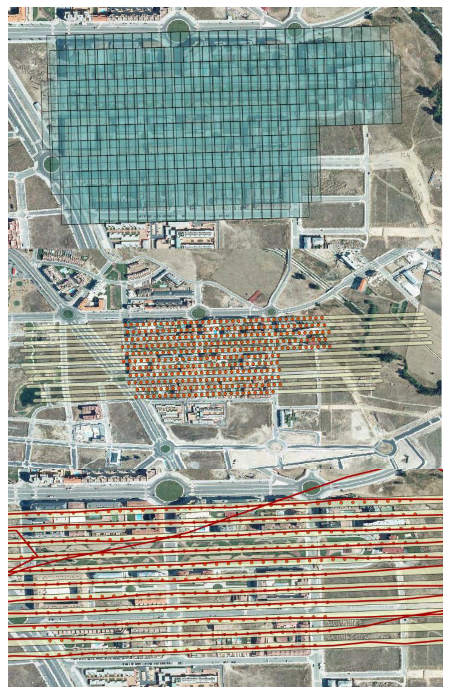
2.2.1. Flight Planning and Data Acquisition
2.2.2. 3D Point Cloud Reconstruction
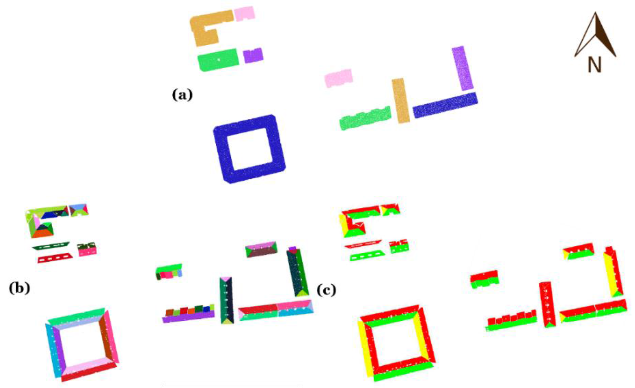
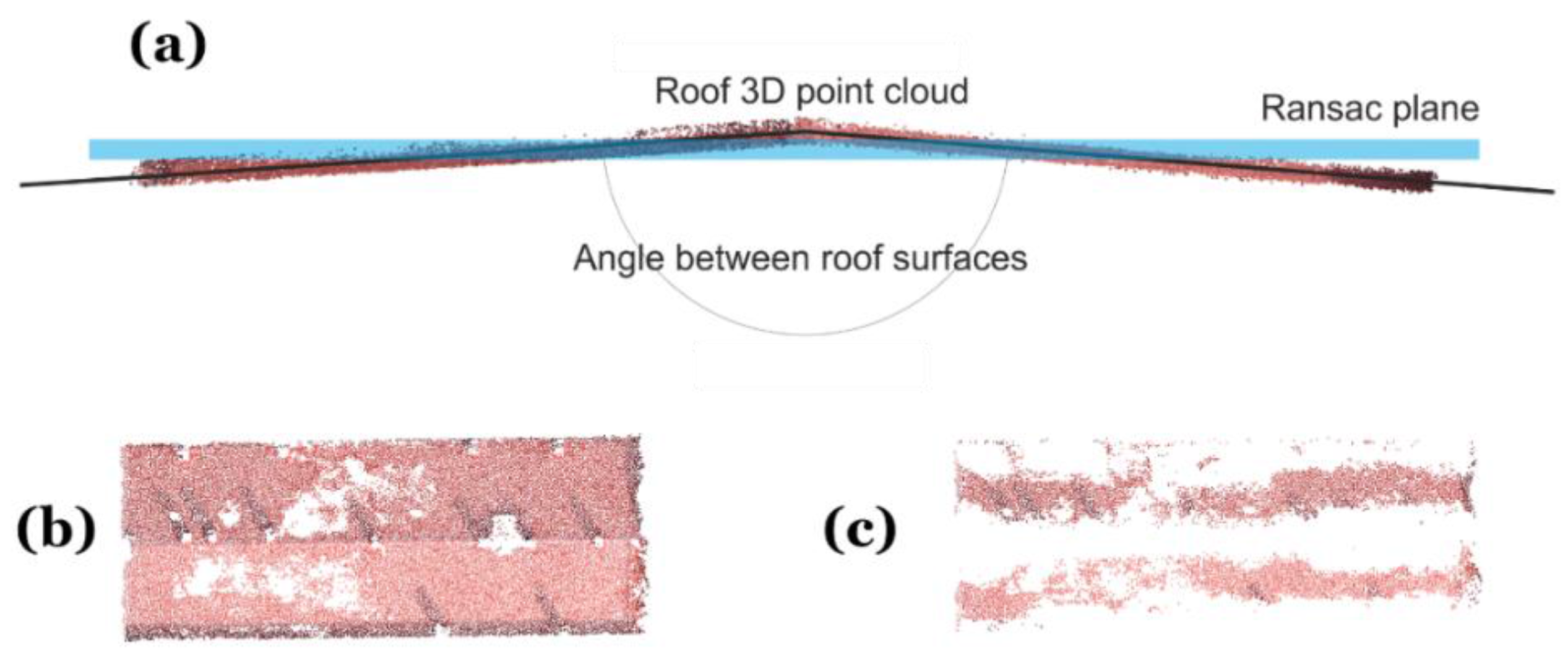
2.2.3. Automatic Planes Segmentation


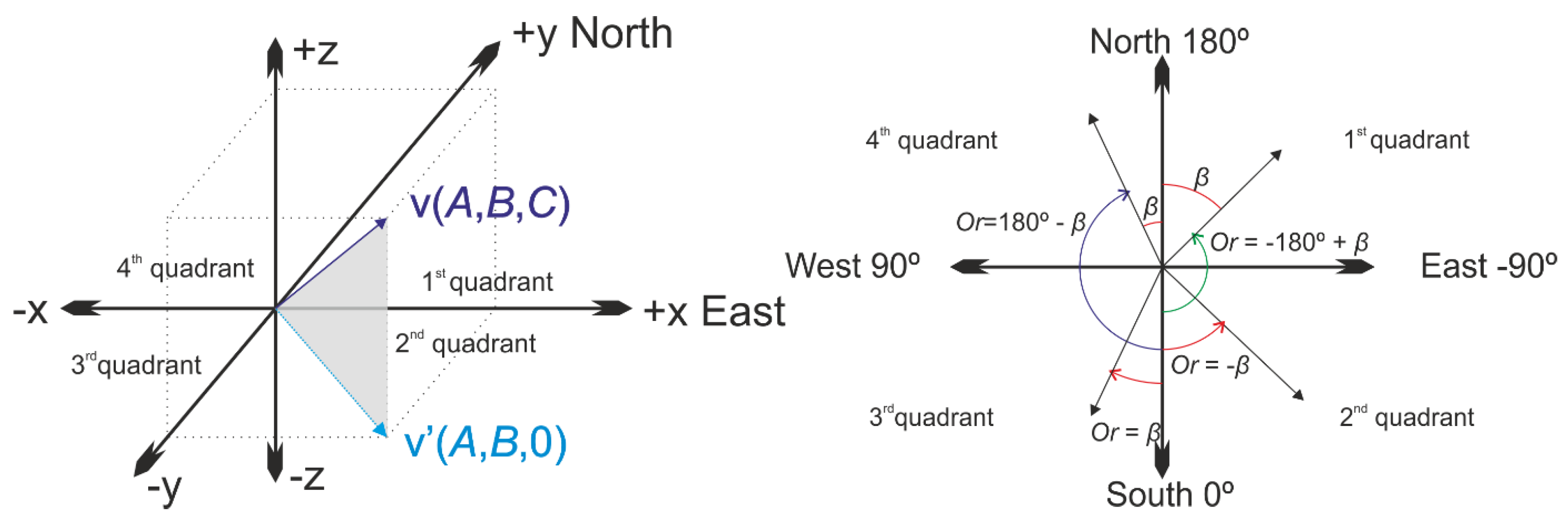
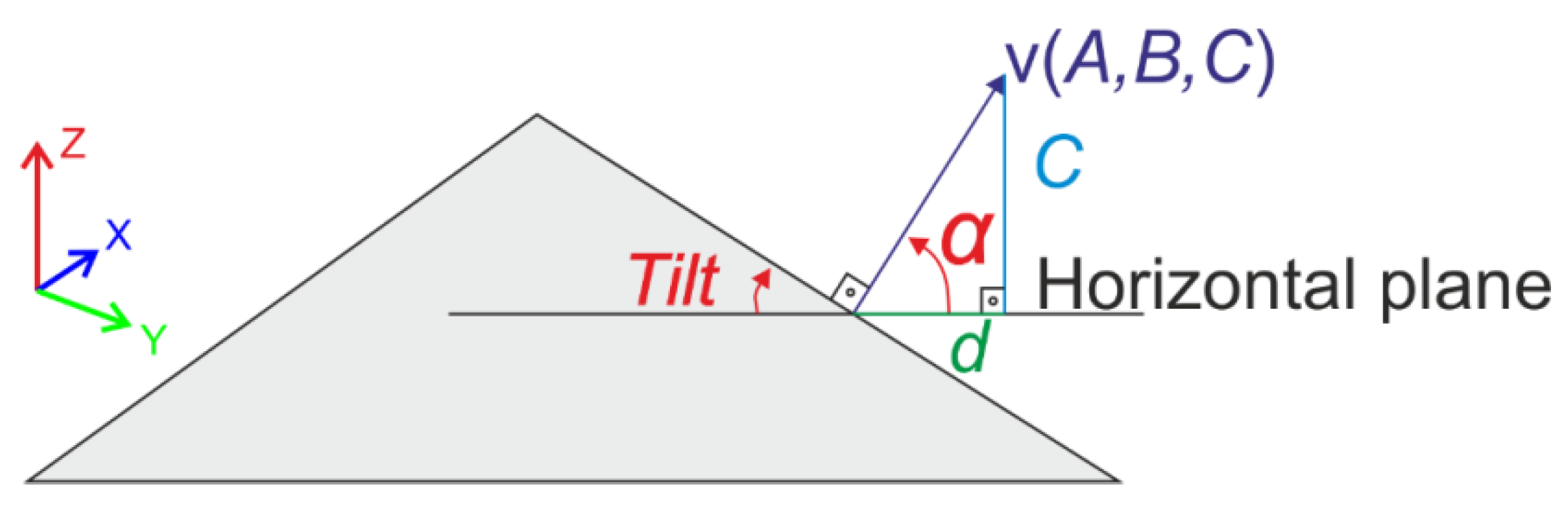
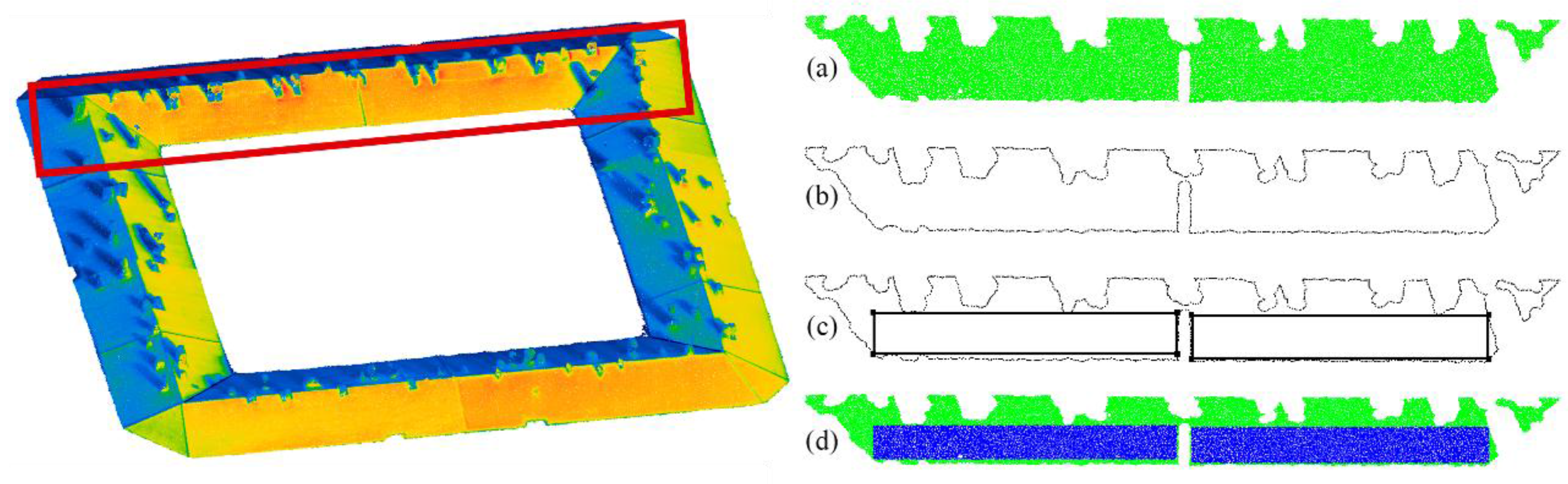
2.2.4. Geometric Analysis and Classification
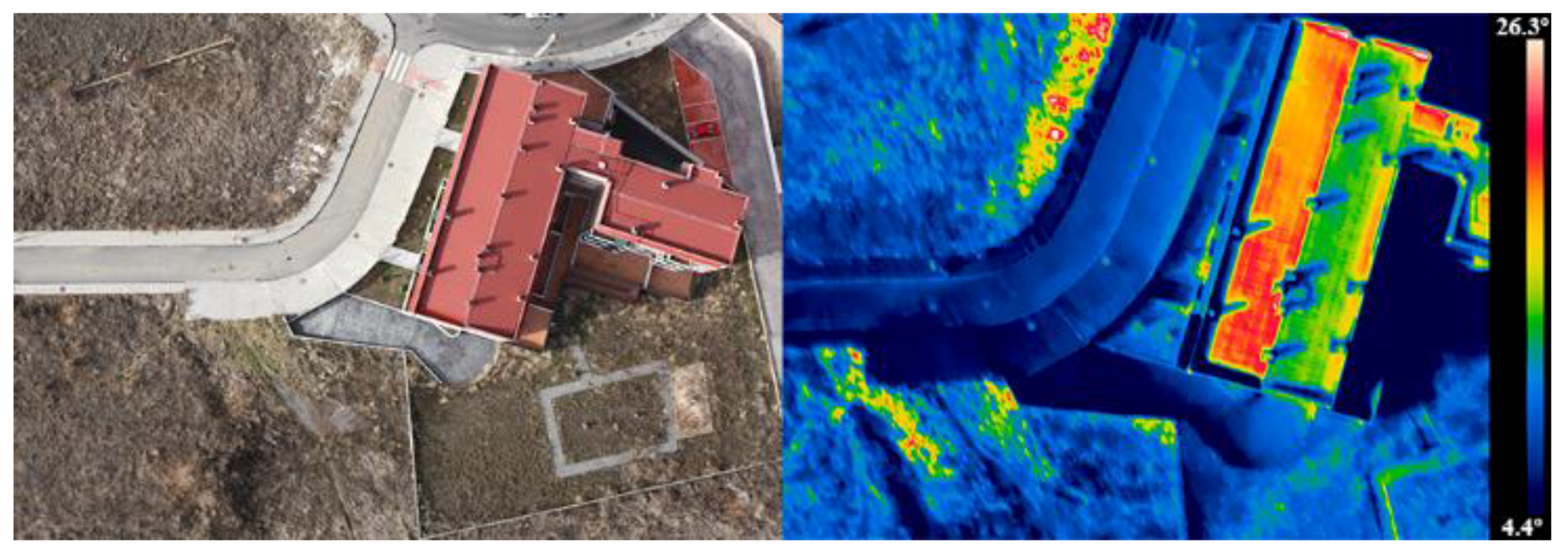
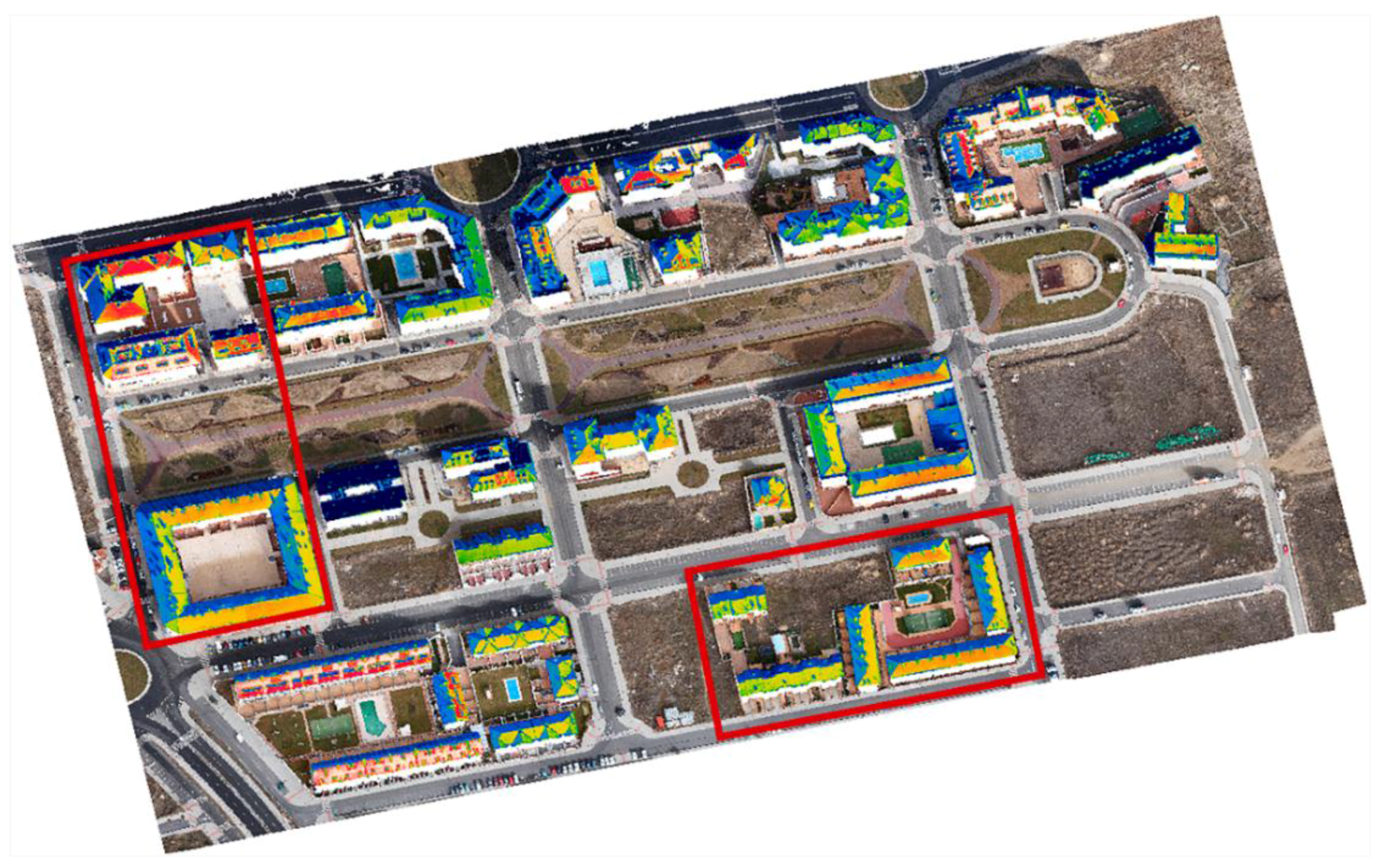
2.2.5. Thermographic Refinement of Surfaces
2.2.6. Location of the Most Suitable Zones
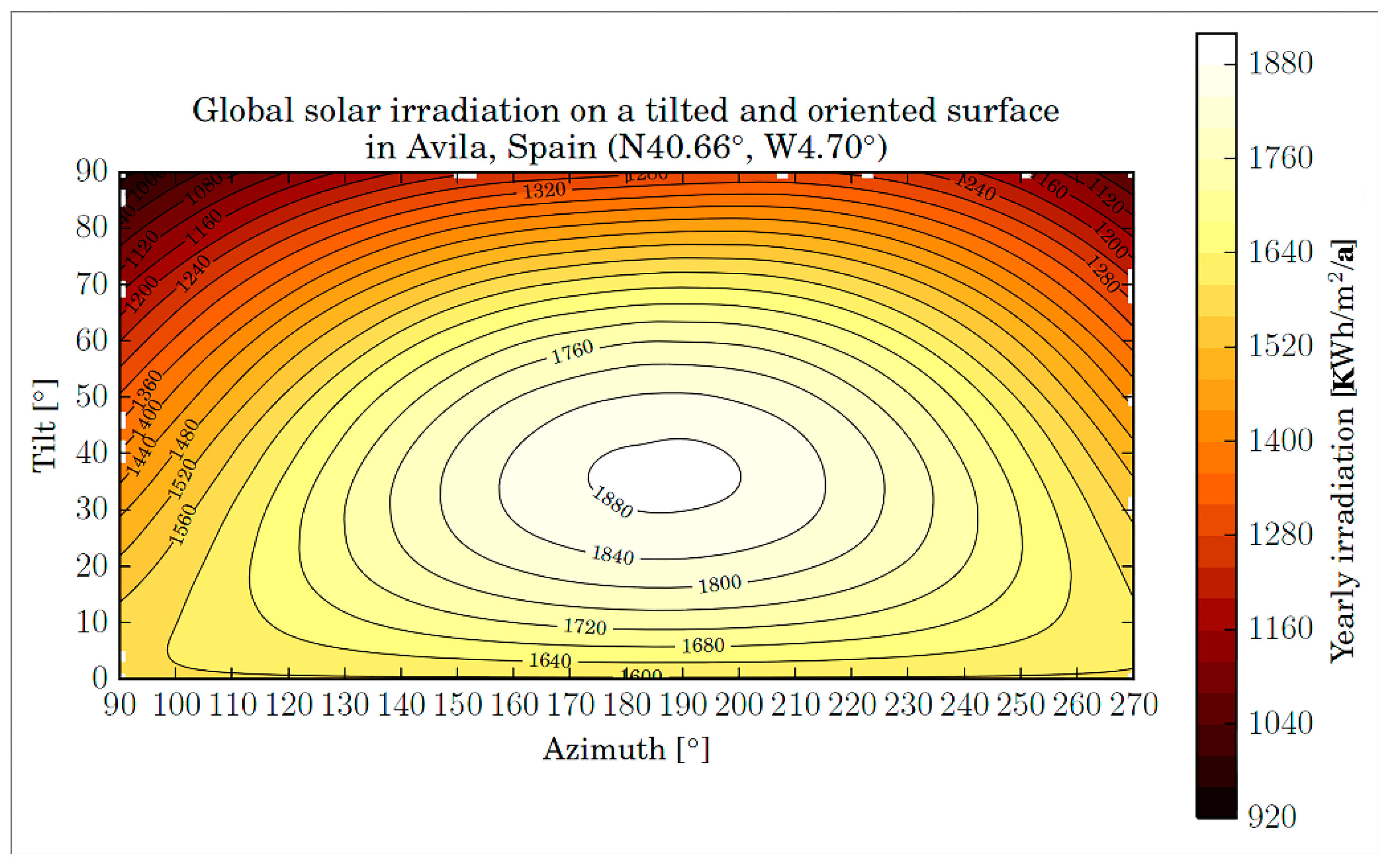
2.2.7. Estimation of the Solar Irradiation
3. Experimental Results
3.1. Study Case


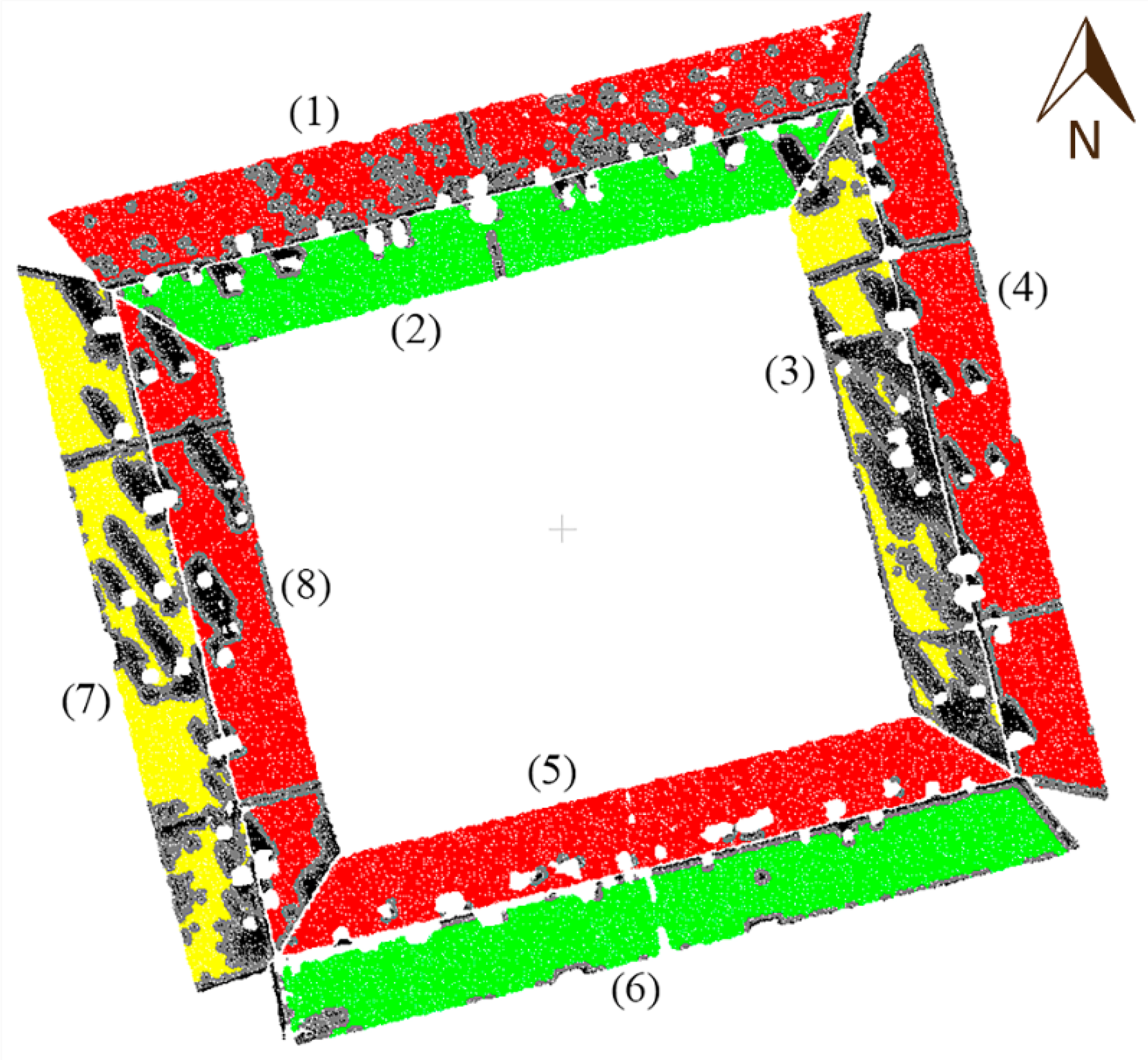

| Surface | Tilt (°) | Azimuth (°) | Yearly Solar Irradiation by m2 (kWh/m2/a) | Area of Optimal Location (m2) | Yearly Total Solar Irradiation (kWh/a) |
|---|---|---|---|---|---|
| 1 | 19.3568 | 346.0080 | 1295.011 | -- | -- |
| 2 | 19.4968 | 165.6463 | 1824.290 | 103.066 | 188,023 |
| -- | -- | -- | -- | 99.026 | 180,652 |
| -- | -- | -- | -- | 18.197 | 33,196.8 |
| 3 | 19.0947 | 156.1201 | 1651.910 | 22.938 | 37,891.8 |
| 4 | 19.3133 | 76.2060 | 1523.485 | -- | -- |
| 5 | 19.2929 | 346.1950 | 1295.834 | -- | -- |
| 6 | 19.5358 | 166.1320 | 1824.914 | 140.417 | 256,249.0 |
| -- | -- | -- | -- | 110.023 | 200,782.0 |
| -- | -- | -- | -- | 41.781 | 76,245.8 |
| -- | -- | -- | -- | 25.003 | 45,628.7 |
| 7 | 19.3667 | 156.0211 | 1652.508 | 38.410 | 63,472.9 |
| 8 | 19.2102 | 76.2400 | 1524.167 | -- | -- |
| Total results for optimal locations of surface 2 | 220.289 | 401,871.8 | |||
| Total results for optimal locations of surface 3 | 22.938 | 37,891.8 | |||
| Total results for optimal locations of surface 6 | 317.224 | 578,905.5 | |||
| Total results for optimal locations of surface 7 | 76.703 | 126,752.5 | |||
| Total results for optimal locations of the roof | 637.154 | 1,145,421.6 | |||

3.2. Computing Efficiency Analysis
4. Conclusions
Acknowledgments
Author Contributions
Conflicts of Interest
References
- Agugiaro, G.; Remondino, F.; Stevanato, G.; De Filippi, R.; Furlanello, C. Estimation of solar radiation on building roofs in mountainous areas. In Procceedings of the ISPRS Conference, Munich, Germany, 5–7 October 2011; pp. 155–160.
- Agugiaro, G.; Nex, F.; Remondino, F.; de Filippi, R.; Droghetti, S.; Furlanello, C. Solar radiation estimation on building roofs and web-based solar cadastre. ISPRS Ann. Photogramm. Remote Sens. Spat. Inf. Sci. 2012, 1, 177–182. [Google Scholar] [CrossRef]
- Hofierka, J.; Suri, M. The solar radiation model for open source gis: Implementation and applications. In Proceedings of the Open Source GIS-GRASS Users Conference, Trento, Italy, 11–13 September 2002; pp. 1–19.
- Nguyen, H.; Pearce, J.M. Estimating potential photovoltaic yield with r. Sun and the open source geographical resources analysis support system. Sol. Energy 2010, 84, 831–843. [Google Scholar] [CrossRef]
- Biljecki, F.; Heuvelink, G.B.M.; Ledoux, H.; Stoter, J. Propagation of positional error in 3D GIS: Estimation of the solar irradiation of building roofs. Int. J. Geogr. Inf. Sci. 2015. [Google Scholar] [CrossRef]
- Strzalka, A.; Alam, N.; Duminil, E.; Coors, V.; Eicker, U. Large scale integration of photovoltaics in cities. Appl. Energy 2012, 93, 413–421. [Google Scholar] [CrossRef]
- Christensen, C.; Barker, G. Effects of tilt and azimuth on annual incident solar radiation for united states locations. In Procceedings of the Solar Forum 2001: Solar Energy: The Power to Choose, Washington, DC, USA, 21–25 April 2001; pp. 225–232.
- López, L.; Lagüela, S.; Picon, I.; González-Aguilera, D. Automatic analysis and classification of the roof surfaces for the installation of solar panels using a multi-data source and multi-sensor aerial platform. Int. Arch. Photogramm. Remote Sens. Spat. Inf. Sci. 2015, 1, 171–178. [Google Scholar] [CrossRef]
- IDAE. Available online: http://www.Idae.Es/uploads/documentos/documentos_5654_fv_pliego_condiciones_tecnicas_instalaciones_conectadas_a_red_c20_julio_2011_3498eaaf.Pdf (accessed on 12 January 2015).
- Microlight Navigation. Available online: http://www.boe.es/diario_boe/txt.php?id=BOE-A-1986-11068 (accessed on 12 January 2015).
- Premerlani, W.; Bizard, P. Direction Cosine Matrix IMU: Theory; DIY Drone: Washington, DC, USA, 2009. [Google Scholar]
- Lagüela, S.; González-Jorge, H.; Armesto, J.; Herráez, J. High performance grid for the metric calibration of thermographic cameras. Meas. Sci. Technol. 2012, 23. [Google Scholar] [CrossRef]
- Kraus, K.; Waldhäusl, P. Photogrammetry: Fundamentals and Standard Processes; Dümmmler Verlag: Bonn, Germany, 1993. [Google Scholar]
- Agarwal, S.; Furukawa, Y.; Snavely, N.; Simon, I.; Curless, B.; Seitz, S.M.; Szeliski, R. Building rome in a day. Commun. ACM 2011, 54, 105–112. [Google Scholar] [CrossRef]
- Lowe, D.G. Object recognition from local scale-invariant features. In Proceedings of the Seventh IEEE International Conference on Computer Vision, Kerkyra, Greece, 20–27 September 1999; pp. 1150–1157.
- Luhmann, T.; Robson, S.; Kyle, S.; Harley, I. Close Range Photogrammetry: Principles, Methods and Applications; Whittles: Dunbeath, UK, 2006. [Google Scholar]
- Deseilligny, M.P.; Clery, I. Apero, an open source bundle adjusment software for automatic calibration and orientation of set of images. In Procceedings of the International Archives of the Photogrammetry, Remote Sensing and Spatial Information Sciences, Trento, Italy, 2–4 March 2011; pp. 269–276.
- Apero-Micmac. Available online: http://www.tapenade.gamsau.archi.fr/TAPEnADe/Tools.html (accessed on 18 June 2015).
- Gehrke, S.; Morin, K.; Downey, M.; Boehrer, N.; Fuchs, T. Semi-global matching: An alternative to lidar for DSM generation. In Proceedings of the 2010 Canadian Geomatics Conference and Symposium of Commission I, Calgary, AB, Canada, 15–18 June 2010.
- Hirschmuller, H. Accurate and efficient stereo processing by semi-global matching and mutual information. In Procceedings of the IEEE Computer Society Conference on Computer Vision and Pattern Recognition, San Diego, CA, USA, 20–25 June 2005; pp. 807–814.
- Gonzalez-Aguilera, D.; Guerrero, D.; Hernandez-Lopez, D.; Rodriguez-Gonzalvez, P.; Pierrot, M.; Fernandez-Hernandez, J. Silver CATCON award, technical commission WG VI/2. In Proceeding of the XXII ISPRS Congress, Melbourne, Australia, 25 August–1 September 2012.
- Rusu, R.B.; Cousins, S. 3D is here: Point cloud library (pcl). In Proceedings of the 2011 IEEE International Conference on Robotics and Automation (ICRA), Shanghai, China, 9–13 May 2011.
- Gallo, O.; Manduchi, R.; Rafii, A. Cc-ransac: Fitting planes in the presence of multiple surfaces in range data. Pattern Recognit. Lett. 2011, 32, 403–410. [Google Scholar] [CrossRef]
- Hulik, R.; Spanel, M.; Smrz, P.; Materna, Z. Continuous plane detection in point-cloud data based on 3D hough transform. J. Vis. Commun. Image Represent. 2014, 25, 86–97. [Google Scholar] [CrossRef]
- Fischler, M.A.; Bolles, R.C. Random sample consensus: A paradigm for model fitting with applications to image analysis and automated cartography. Commun. ACM 1981, 24, 381–395. [Google Scholar] [CrossRef]
- Edelsbrunner, H.; Kirkpatrick, D.G.; Seidel, R. On the shape of a set of points in the plane. IEEE Trans. Inf. Theory 1983, 29, 551–559. [Google Scholar] [CrossRef]
- Orlowski, M. A new algorithm for the largest empty rectangle problem. Algorithmica 1990, 5, 65–73. [Google Scholar] [CrossRef]
- Yang, H.; Lu, L. The optimum tilt angles and orientations of pv claddings for building-integrated photovoltaic (BIPV) applications. J. Sol. Energy Eng. 2007, 129, 253–255. [Google Scholar] [CrossRef]
- Santos, T.; Gomes, N.; Freire, S.; Brito, M.; Santos, L.; Tenedório, J. Applications of solar mapping in the urban environment. Appl. Geogr. 2014, 51, 48–57. [Google Scholar] [CrossRef]
- Li, Z.; Zhang, Z.; Davey, K. Estimating geographical pv potential using lidar data for buildings in downtown san francisco. Trans. GIS 2015. [Google Scholar] [CrossRef]
- Šúri, M.; Hofierka, J. A new GIS-based solar radiation model and its application to photovoltaic assessments. Trans. GIS 2004, 8, 175–190. [Google Scholar] [CrossRef]
- Liang, J.; Gong, J.; Li, W.; Ibrahim, A.N. A visualization-oriented 3D method for efficient computation of urban solar radiation based on 3D–2D surface mapping. Int. J. Geogr. Inf. Sci. 2014, 28, 780–798. [Google Scholar] [CrossRef]
- Gulin, M.; Vašak, M.; Perić, N. Dynamical optimal positioning of a photovoltaic panel in all weather conditions. Appl. Energy 2013, 108, 429–438. [Google Scholar] [CrossRef]
- Masters, G.M. Renewable and Efficient Electric Power Systems; John Wiley & Sons Inc.: Hoboken, NJ, USA, 2013. [Google Scholar]
- David, M.; Lauret, P.; Boland, J. Evaluating tilted plane models for solar radiation using comprehensive testing procedures, at a southern hemisphere location. Renew. Energy 2013, 51, 124–131. [Google Scholar] [CrossRef]
- Demain, C.; Journée, M.; Bertrand, C. Evaluation of different models to estimate the global solar radiation on inclined surfaces. Renew. Energy 2013, 50, 710–721. [Google Scholar] [CrossRef]
- Gulin, M.; Vašak, M.; Baotic, M. Estimation of the global solar irradiance on tilted surfaces. In Proceedings of the 17th International Conference on Electrical Drives and Power Electronics (EDPE 2013), Dubrovnik, Hrvatska, 2–4 October 2013; pp. 334–339.
- Solar3Dcity. Available online: https://github.com/tudelft3d/Solar3Dcity (accessed on 5 August 2015).
- Energy Plus weather data. Available online: http://apps1.eere.energy.gov/buildings/energyplus/weatherdata_about.cfm (accessed on 5 August 2015).
- XEphem. Available online: http://www.clearskyinstitute.com/xephem/ (accessed on 5 August 2015).
- Meeus, J.H. Astronomical Algorithms; Willmann-Bell, Incorporated: Richmond, VA, USA, 1991. [Google Scholar]
- Reda, I.; Andreas, A. Solar position algorithm for solar radiation applications. Sol. Energy 2004, 76, 577–589. [Google Scholar] [CrossRef]
- Perez, R.; Ineichen, P.; Seals, R.; Michalsky, J.; Stewart, R. Modeling daylight availability and irradiance components from direct and global irradiance. Sol. Energy 1990, 44, 271–289. [Google Scholar] [CrossRef]
- Solpy. Available online: https://github.com/nrcharles/solpy (accessed on 5 August 2015).
- Šúri, M.; Huld, T.A.; Dunlop, E.D. Pv-gis: A web-based solar radiation database for the calculation of pv potential in europe. Int. J. Sustain. Energy 2005, 24, 55–67. [Google Scholar] [CrossRef]
- Rowlands, I.H.; Kemery, B.P.; Beausoleil-Morrison, I. Optimal solar-pv tilt angle and azimuth: An Ontario (Canada) case-study. Energy Policy 2011, 39, 1397–1409. [Google Scholar] [CrossRef]
- PNOA. Available online: https://contrataciondelestado.es/wps/wcm/connect/7050f80e-1d0c-4231-afad-5c8262529580/DOC20090605131632pdf.pdf?MOD=AJPERES (accessed on 16 August 2015).
- LiDar Data. Available online: http://centrodedescargas.cnig.es/CentroDescargas/buscadorCatalogo.do?codFamilia=LIDAR (accessed on 12 August 2015).
© 2015 by the authors; licensee MDPI, Basel, Switzerland. This article is an open access article distributed under the terms and conditions of the Creative Commons Attribution license (http://creativecommons.org/licenses/by/4.0/).
Share and Cite
López-Fernández, L.; Lagüela, S.; Picón, I.; González-Aguilera, D. Large Scale Automatic Analysis and Classification of Roof Surfaces for the Installation of Solar Panels Using a Multi-Sensor Aerial Platform. Remote Sens. 2015, 7, 11226-11248. https://doi.org/10.3390/rs70911226
López-Fernández L, Lagüela S, Picón I, González-Aguilera D. Large Scale Automatic Analysis and Classification of Roof Surfaces for the Installation of Solar Panels Using a Multi-Sensor Aerial Platform. Remote Sensing. 2015; 7(9):11226-11248. https://doi.org/10.3390/rs70911226
Chicago/Turabian StyleLópez-Fernández, Luis, Susana Lagüela, Inmaculada Picón, and Diego González-Aguilera. 2015. "Large Scale Automatic Analysis and Classification of Roof Surfaces for the Installation of Solar Panels Using a Multi-Sensor Aerial Platform" Remote Sensing 7, no. 9: 11226-11248. https://doi.org/10.3390/rs70911226