Modifying Geometric-Optical Bidirectional Reflectance Model for Direct Inversion of Forest Canopy Leaf Area Index

Abstract

Forest canopy leaf area index (LAI) inversion based on remote sensing data is an important method to obtain LAI. Currently, the most widely-used model to achieve forest canopy structure parameters is the Li-Strahler geometric-optical bidirectional reflectance model, by considering the effect of crown shape and mutual shadowing, which is referred to as the GOMS model. However, it is difficult to retrieve LAI through the GOMS model directly because LAI is not a fundamental parameter of the model. In this study, a gap probability model was used to obtain the relationship between the canopy structure parameter nR² and LAI. Thus, LAI was introduced into the GOMS model as an independent variable by replacing nR² The modified GOMS (MGOMS) model was validated by application to Dayekou in the Heihe River Basin of China. The LAI retrieved using the MGOMS model with optical multi-angle remote sensing data, high spatial resolution images and field-measured data was in good agreement with the field-measured LAI, with an R-square (R²) of 0.64, and an RMSE of 0.67. The results demonstrate that the MGOMS model obtained by replacing the canopy structure parameter nR² of the GOMS model with LAI can be used to invert LAI directly and precisely.

1. Introduction

Leaf Area Index (LAI) is defined as the one-sided green leaf area per unit of horizontal ground surface area [1]; it is an important botany parameter in the study of farming [2,3,4,5,6,7], forestry [8,9], climate of meteorology [10], and ecology [11]. Forest ecosystems are essential parts of the terrestrial ecosystem, and the LAI inversion of forest canopy is one of the main objects of forest ecosystem research [12,13,14,15]. Due to complex terrain, variable weather conditions, limited field-measured data, and uneven vegetation types, among other factors, the inversion and verification of forest LAI are usually difficult.

Methods of obtaining LAI include field measurements, photography simulations [16,17], and model inversion using semi-empirical [8,18,19] or physical models; in particular, model inversion using physical models is the most widely-used method to achieve forest canopy LAI. The earliest practical canopy reflectance model was determined by Suits [20,21]. Verhoef [22] then extended the Suits model by considering the influence of the leaf-angle distribution, to create the SAIL model. The SAIL model can simplify the description of canopy structures. Reyna and Bhadwar [23] later considered the influence of specular reflection. Among all the canopy LAI inversion models, the canopy geometric-optical (GO) model has attracted a lot of interest. The earliest GO model was produced in the mid-1970s [24,25,26]. The GO model fully considers the macroscopic geometric structure of the objects and assumes that the objects are geometries with a specific arrangement and known geometric shapes and optical properties. According to the geometric optical principles, the GO model can analyze the influences of the interception, shielding of the incident light, and surface reflection, and determine the directional reflectance of the vegetation canopy. Based on the “scene synthesis model”, the GO model considers four components, including sunlit leaf or canopy, shaded leaf or canopy, sunlit background, and shaded background, and establishes the bidirectional reflectance distribution function (BRDF) model under different illumination and observation conditions. In 1985 and 1986, Li and Strahler applied the GO model to remote sensing data using a simple cone model instead of the tree canopy [27,28]. In the past, many attempts to optimize the GO model have been made. For example, Schaaf et al. [29] built a geometric optical model that considered terrain factors. Qi et al. [30] combined the statistical model with the optical model, which gives a more accurate estimation of LAI. In order to apply the model to the dense forest, earlier studies [31,32,33] proposed the geometric-optical mutual shadowing (GOMS) model which considers the effects of mutual shadowing and the radiation transfer process [34], and expanded it to the thermal radiation [35], making the GOMS model the most representative GO model.

GO models considering the object and the atmospheric scattering are suitable for discontinuous vegetation (e.g., shrubbery, sparse forests, coniferous forests, and orchards) and rough surfaces for which the radiation transfer model is difficult to apply. The Li-Strahler GOMS model is a pixel-scale GO model which considers the effects of topographic factors. This model can successfully establish the relationship between forest structure parameters (e.g., average vegetation coverage, average tree height, crown size) and the canopy bidirectional reflection distribution function, giving the relationship between the canopy structure parameters (e.g., clear height, crown radius, forest canopy distribution) and the canopy reflection characteristics [28,31]. LAI is not an independent parameter in GOMS. Hence, in previous studies [36,37], crown center height (h), horizontal radius (R) or other parameters were firstly retrieved in the GOMS model. Then, canopy LAI was obtained by the statistical relationship between the field-measured h, R or other parameters and the field-measured LAI. However, this calculated process is very complicated and the accuracy of the retrieved LAI depends on the precision of the field-measured parameters. To address this problem, the GOMS model was improved in the present study by introducing LAI into the model to enable direct inversion of LAI via the modified GOMS (i.e., MGOMS) model. The GOMS model consists of the canopy structure parameter ${\text{nR}}^2$, a parameter that describes the crown coverage condition in the nadir observation. Since LAI and ${\text{nR}}^2$ are both functions of area and are not dependent on the viewing angle, in this paper, the gap probability model is used to build the relationship between LAI and ${\text{nR}}^2$. Then, LAI is introduced into the GOMS model by replacing ${\text{nR}}^2$ with LAI. The accuracy of the MGOMS model is demonstrated using field-measured and remote sensing datasets.

2. Data and Pre-Processing

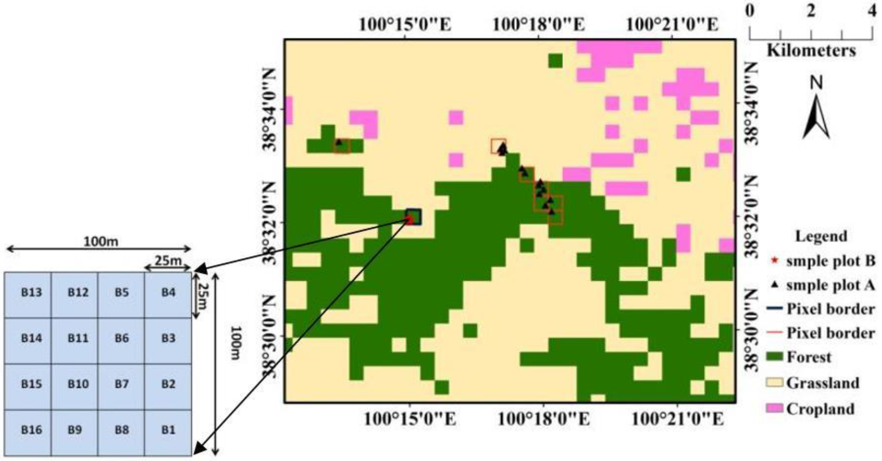
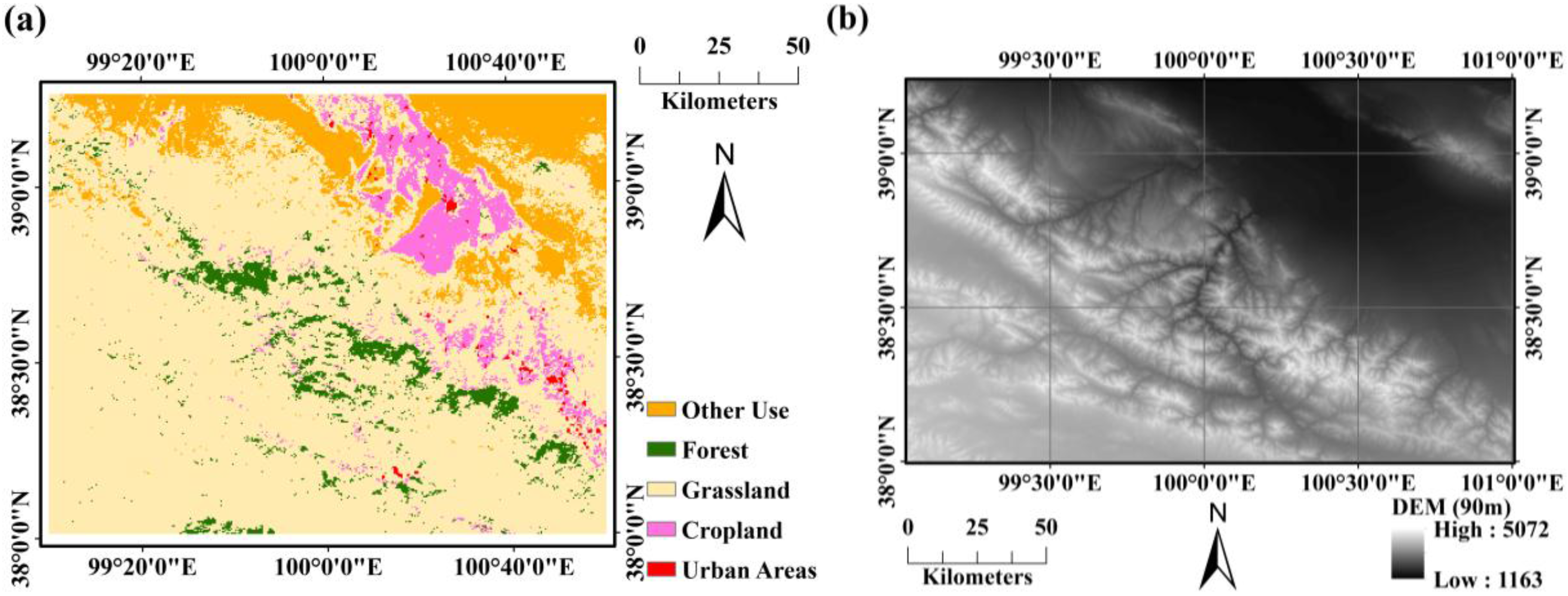
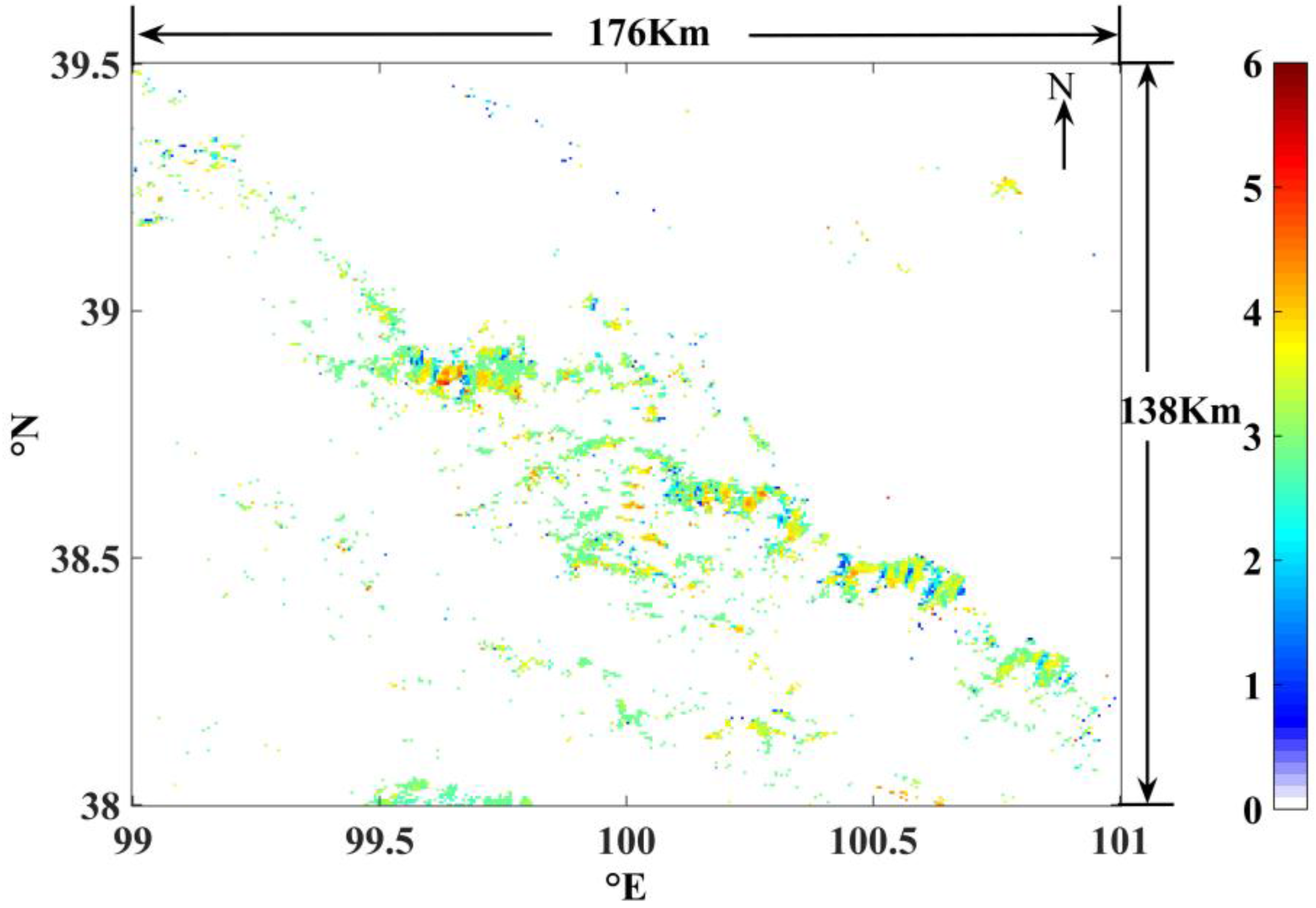
2.1. Study Area

In our study, the study site Dayekou forest (100°E, 38.6°N) is located in the Qilian Mountain area, Gansu Province of China. The Heihe Basin is the second largest inland river basin of the arid region in Northwest China, the annual precipitation in the middle valley is 140 mm [38] and mainly occurs in the summer. Its ecological system is particularly fragile. Dayekou is located in the middle valley of the Heihe River basin and is mostly covered by forest and upland meadow. The main vegetation types in Dayekou are Picea crassifolia, shrubland, and upland meadow, and the dominant forest type is P. crassifolia. The MODIS land cover product (MCD12Q1) was used to select forest pixels. The forest pixels are indicated in green in Figure 1a.

Figure 1. (a) Dayekou land-cover type from the MODIS land-cover product. The spatial resolution is 500 m. Pixels in green, pale yellow, pink, and red are forest pixels, grassland pixels, cropland pixels, and urban areas, respectively. Pixels in brown yellow represent land for other use; (b) Digital Elevation Map (DEM) map of Dayekou. The size of the map is the same as that in Figure 1a. The spatial resolution is 90 m. In this map, altitude generally increased with decreasing latitude and longitude.

Figure 1. (a) Dayekou land-cover type from the MODIS land-cover product. The spatial resolution is 500 m. Pixels in green, pale yellow, pink, and red are forest pixels, grassland pixels, cropland pixels, and urban areas, respectively. Pixels in brown yellow represent land for other use; (b) Digital Elevation Map (DEM) map of Dayekou. The size of the map is the same as that in Figure 1a. The spatial resolution is 90 m. In this map, altitude generally increased with decreasing latitude and longitude.

The locations of the field measurement sample plots are shown in Figure 2. There were 30 field measurement sample plots in the Dayekou site, including 15 sample plots “A” with a size of 20 m × 20 m and 16 sample plots “B” with a size of 25 m × 25 m. However, in Section 4.2.3, sample plot B10 is not included because there was no field-measured LAI in this sample plot. The B sample plots were part of a super sample plot. The super sample plot was 100 m × 100 m in size located within the black line surrounding the pixels and was divided into 16 parts. In this super sample plot, all parameters related to trees were measured, including LAI and canopy structure parameters. The field-measured canopy structure parameters measured in these sample plots are described in Section 2.2.1. Both A and B sample plots are relatively homogeneous sample plots which can represent the real condition at the 500-m pixel scale, and the dominant tree species in them is Picea crassifolia.

Figure 2. Sample plot locations in our study area in the MODIS land-cover products. Pixels where the A sample plots were located are outlined in red, and the pixels where the B sample plots were located are outlined in black. B sample plots are the part of a super sample plot.

Figure 2. Sample plot locations in our study area in the MODIS land-cover products. Pixels where the A sample plots were located are outlined in red, and the pixels where the B sample plots were located are outlined in black. B sample plots are the part of a super sample plot.

2.2. Data Foundation

All the data used in this article were obtained from the Heihe Watershed Allied Telemetry Experimental Research (HiWATER), the field-measured data in the B sample plots were collected at the Dayekou Guantan forest station (100°15′E, 38°32′N), Heihe river basin, China [39].

2.2.1. Field-Measured Data

Field measurements were performed during June 2008 in the field measurement sample plots. Tracing Radiation and Architecture of Canopies (TRAC, Natural Resources Canada, Canada Centre for Remote Sensing, Saint-Hubert, QC, Canada) [40] and LAI-2000 Plant Canopy Analyzer (LAI-2000, LI-COR Inc, Lincoln, NE, USA) [41] were used to measure LAI of each sample plot [42]. LAI-2000 was used to measure the effective LAI (${\text{LAI}}_{\text{e}}$), and TRAC was used to measure both the effective LAI (${\text{LAI}}_{\text{e}}$) and the foliage clumping index ($\text{Ω}$). The true LAI of each sample plot was obtained through the equation ${\text{LAI}}_{\text{t}}$ = ${\text{LAI}}_{\text{e}}$/$\text{Ω}$. The field-measured LAI was used to validate the inversion efficiency of the model.

In addition, the forest canopy structural parameters of each tree were measured in the B sample plots. The measured geometrical structural parameters included tree horizontal radius of the tree crown (R), tree height (H), clear bole height (h), and the diameter at breast height (DBH). The tree height of each tree in the B sample plots was measured by laser altimeter (TruPulse 200, Laser Technology Inc. (LTI), Norristown, PA, USA). The field-measured data was used to provide prior knowledge of the canopy structure parameters in the GOMS and MGOMS models.

The protocols for each instrument used in the sample plots and the sample plot layouts were described in detail in a previous study [37].

2.2.2. MODIS, MISR, and SPOT Reflectance Data

In the inversion process, optical multi-angle remote sensing data and high spatial resolution images were used to do the research. Moderate-resolution Imaging Spectro Radiometer (MODIS) and Multi-angle Imaging SpectroRadiometer (MISR) reflectance products were used to provide the multi-angle bidirectional reflectance datasets in this study. SPOT-5 data was used to provide the spectral information.

Ten images of MODIS 500-m daily bidirectional surface reflectance data (MOD09GA) spanning a MODIS 16-day observation period (Figure 3), were selected in the validation process. MODIS 500-m 8-day bidirectional surface reflectance data (MOD09A1) and MISR 1-km bidirectional surface reflectance data, spanning 1 May–28 July 2008, were selected to build the BRF datasets. The BRF datasets were constructed as follows. First, the MISR BRF and MODIS BRF data projections were transferred into UTM, WGS84. Second, the spatial resolutions of the MISR and MODIS data were normalized by dividing each of the MISR pixels into four 500 m pixels with the same BRF value and viewing direction. Third, the bidirectional reflectance and geometric information, including sun zenith angle and azimuth, viewing zenith angle and azimuth of each pixel, were extracted to build the BRF dataset both in the red and near-infrared (NIR) bands. The BRF datasets were used as the input parameters of the model inversion procedure. The main data processing procedures to construct the BRF dataset were explained in detail in a previous study [36].

Figure 3. Solar position and view position of the selected MOD09GA datasets in uncertainty and sensitivity analysis processes. The datasets span a MODIS 16-day observation period. The numbers 154–177 are the DOY of the MODIS BRF products in 2008.

Figure 3. Solar position and view position of the selected MOD09GA datasets in uncertainty and sensitivity analysis processes. The datasets span a MODIS 16-day observation period. The numbers 154–177 are the DOY of the MODIS BRF products in 2008.

The SPOT-5 multi-band image obtained on 10 August 2008 that covers the study site was used to obtain information on the four component spectra (G, C, Z, T). The spatial resolution of this SPOT-5 data was 10 m. The FLASSH model [43] was used for atmospheric correction of the SPOT-5 image. As noted by Fu et al. [37], the incident radiation was inconsistent during the measuring process. Hence, we cannot obtain the available spectra of the components from field measurements. Using the four components spectra obtained from remote sensing data with high spatial resolution images can reduce the uncertainty due to scaling effects. Moreover, after the atmospheric correction of the SPOT-5 remote sensing images, the incident radiation can be considered consistent within a MODIS pixel. Thus, we chose the SPOT-5 data instead of the field-measured radiation data to provide the required spectral information.

2.2.3. Airborne LiDAR data

LiDAR data were used to support the canopy height model (CHM) in our study. The LiDAR data we used were acquired on 28 June 2008, using a laser scanner (Riegl LMS-Q560, Riegl, Horn, Austria) with a maximum scan angle of ±0.5 mrad from nadir. The raw LiDAR data were processed using Terrasolid software (Terrasolid software (Version 007), Terrasolid Ltd., Helsinki, Finland) to classify the data into two types: ground points and non-ground points. The DEM was built from ground points, and the digital surface model (DSM) was produced from non-ground points. Then, the CHM was created with a resolution of 0.5 m by subtracting the DEM from the DSM. The CHM was used to provide b and ${\text{nR}}^2$ in Section 4.2.3.

3. Method

3.1. Theoretical Foundation

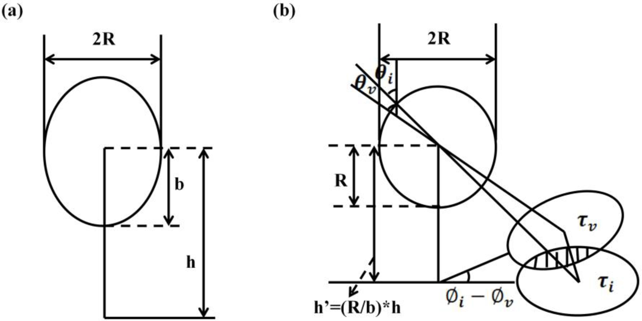
3.1.1. Geometric-Optic Mutual Shadowing Model

The GOMS model is constructed based on the Li-Strahler geometric-optical model, which considers the mutual shadowing of crowns and makes the geometric optic model more suitable for highly dense canopy forests [31].

The assumption of the GOMS model is that the reflectance of a pixel can be modeled as a sum of the reflectances of its individual scene components as weighted by their respective areas within the pixel [28]. The model also assumes that the vegetation canopy BRDF characteristics at the pixel scale can be explained by geometric optical principle when the discontinuous three-dimensional geometry in a pixel is illuminated and observed in different directions. The reflections received by the sensors are the ground reflection and the crown reflection in the field of view A (“A” is only the assumption that the area of the field of view is A). Considering the three-dimensional canopy structure parameters, the influence of sky light and multiple scattering, the received signal can be defined as the combination of four area weighted components:

$$\text{S}={\text{K}}_{\text{g}}G+{\text{K}}_{\text{c}}C+{\text{K}}_{\text{z}}Z +{\text{K}}_{\text{t}}T$$

(1)

where S is bidirectional reflectance; ${\text{K}}_{\text{g}}$, ${\text{K}}_{\text{c}}$, ${\text{K}}_{\text{z}}$, and ${\text{K}}_{\text{t}}$ are the proportions of sunlit background, sunlit crown, shaded background, and shaded crown the GO modeled, respectively; and G, C, Z, and T are the contributions of the sunlit background, sunlit crown, shaded background, and shaded crown, respectively [27,44]. ${\text{K}}_{\text{g}},{\text{ K}}_{\text{c}},{\text{ K}}_{\text{z}},{\text{ and K}}_{\text{t}}$ can be expressed by a combination of the forest canopy structural parameters. We assume that the tree crown shape is ellipsoidal (Figure 4a) and that the forest canopy structure parameters include R (the horizontal radius of an ellipsoidal crown), b (the vertical half axis of an ellipsoidal crown), h (the height at which a crown center is located), and n (the number of crowns per unit area).

Figure 4. (a) Forest canopy shape in ellipsoid. R is the horizontal radius of an ellipsoidal crown, b is the vertical half axis of an ellipsoidal crown, and h is the height at which a crown center is located; (b) Simplified schematic diagram of forest vegetation canopy in the GOMS model [31]. ${\theta }_{\text{i}}$ and ${\theta }_{\text{v}}$ are the revised solar zenith angle and view zenith angle, respectively. ${Ø}_{\text{i}}$ and ${Ø}_{\text{v}}$ are the solar azimuth and view azimuth, respectively. ${Ø}_{\text{i}}-{Ø}_{\text{v}}$ is the azimuthal difference between the illumination and viewing directions. ${\mathrm{\tau }}_{\text{i}}$ and ${\mathrm{\tau }}_{\text{v}}$ are the sunlit shadow and viewed shadow, respectively. The shaded area is the mutual shadowing area of the sunlit shadow and viewed shadow.

Figure 4. (a) Forest canopy shape in ellipsoid. R is the horizontal radius of an ellipsoidal crown, b is the vertical half axis of an ellipsoidal crown, and h is the height at which a crown center is located; (b) Simplified schematic diagram of forest vegetation canopy in the GOMS model [31]. ${\theta }_{\text{i}}$ and ${\theta }_{\text{v}}$ are the revised solar zenith angle and view zenith angle, respectively. ${Ø}_{\text{i}}$ and ${Ø}_{\text{v}}$ are the solar azimuth and view azimuth, respectively. ${Ø}_{\text{i}}-{Ø}_{\text{v}}$ is the azimuthal difference between the illumination and viewing directions. ${\mathrm{\tau }}_{\text{i}}$ and ${\mathrm{\tau }}_{\text{v}}$ are the sunlit shadow and viewed shadow, respectively. The shaded area is the mutual shadowing area of the sunlit shadow and viewed shadow.

When the ellipsoid is stretched in the vertical direction and made b equal to R (Figure 4b), then ${\text{K}}_{\text{g}},{\text{ K}}_{\text{c}},{\text{ K}}_{\text{z}},{\text{ and K}}_{\text{t}}$ can be expressed as:

$${\text{K}}_{\text{g}}=\text{exp}\left(-\text{n * }\left[{\tau }_i+{\tau }_v-\text{O}\left({\theta }_{\text{i}},{\text{ θ}}_{\text{v}},{Ø}_i-{Ø}_v\right)\right]\right)$$

(2)

where

$${\mathrm{\tau }}_{\text{i}}=\pi R^2/\cos {\theta }_{\text{i}}$$

(3)

$${\mathrm{\tau }}_{\text{v}}=\pi R^2/\cos {\theta }_{\text{v}}$$

(4)

and where $\text{O}\left({\theta }_i, {\theta }_v,{Ø}_i-{Ø}_v\right)$ is the shaded area in Figure 4b. ${Ø}_i$ and ${Ø}_v$ are the solar azimuth and view azimuth, but ${\theta }_i$ and ${\theta }_v$ are not the solar zenith angle and view zenith angle yet; they have been revised in the stretching process:

$${\theta }_{\text{i}}={\tan }^{-1}\left(\left(b/R\right)\tan {{\theta }_{\text{i}}}^{\prime }\right)$$

(5)

$${\theta }_{\text{v}}={\tan }^{-1}\left(\left(b/R\right)\tan {{\theta }_{\text{v}}}^{\prime }\right)$$

(6)

where ${{\theta }_i}^{\prime }$ and ${{\theta }_v}^{\prime }$ are solar zenith angle and view zenith angle.

$${\text{K}}_{\text{c}}=1-\text{exp}\left(-\text{n * }\left[\frac{1}{2}\left(1+\overrightarrow{\text{i}},\overrightarrow{\text{v}}\right){\mathrm{\tau }}_{\text{v}}\right]\right)$$

(7)

$${\text{K}}_{\text{t}}=\exp \left(-\text{n * }\left[\frac{1}{2}\left(1+\overrightarrow{\text{i}},\overrightarrow{\text{v}}\right){\mathrm{\tau }}_{\text{v}}\right]\right)-\text{exp}\left(-{\text{n * τ}}_{\text{v}}\right)$$

(8)

$${\text{K}}_{\text{z}}=1-{\text{K}}_{\text{g}}-{\text{K}}_{\text{c}}-{\text{K}}_{\text{t}}$$

(9)

We can simplify the expression of the GOMS model using the function below:

$$\text{S} =\text{f}\left({\theta }_i, {Ø}_i, {\theta }_v, {Ø}_v, {\theta }_s, {Ø}_s, n{R}^2,b/R,h/b,\Delta h/b, G, C, Z,T\right)$$

(10)

where S is bidirectional reflectance; $n{R}^2$ derived from $n*\pi R^2$ which contains the crown density information (n), that represents the crown coverage condition per unit area in the nadir observation; b/R is the crown shape parameter which significantly affects the crown coverage density in the non-nadir direction; h/b is the parameter which represents the crown height from the ground and mainly affects the outward width of the hot spot; $\Delta \text{h}$ is the variance of the h distribution in one pixel; and $\Delta h/b$ is the parameter which describes the discrete degree of the crown height distribution and affects the bowl-shape of the BRDF. ${\theta }_s\text{ and }{Ø}_s$ are the local slope and aspect, respectively [36,37]. ${\theta }_i, {Ø}_i, {\theta }_v,\text{ and }{Ø}_v$ are the solar zenith angle, solar azimuth, view zenith angle, and view azimuth, respectively.

In Equation (10), there are many input parameters in the GOMS model, but LAI is not an independent parameter in the model. We therefore attempt to modify the GOMS model by introducing LAI into Equation (10), that is, S = f(LAI, …), to allow LAI to be retrieved by the modified GOMS model directly.

3.1.2. Gap Probability Model

A gap probability model is a GO model that uses the average transmission theory or the simplified radiation transfer equation to simulate the distribution of the leaves by calculating radiation attenuation and consequently determining the radiation characteristics of the vegetation canopy. The most improved gap probability model is the Li-Strahler Gap probability model [45], in which LAI is an independent parameter.

When considering a unique canopy:

$${\text{P}}_{\text{gap}}(\theta )=\text{exp}\left(-\text{K}(\theta )\text{ * }LAI\text{ * s}/\text{D}\right)=\text{exp}\left(-\text{τs}\right)$$

(11)

where s is the distance traveled by a photon within the canopy; $\mathrm{\tau }=\text{K}(\theta )\text{ * LAI}/\text{D}$ mainly depends on the leaf density and the foliage angle distribution (FAD); K $(\theta )$ is the coefficient of leaf angle distribution function; and D is the average depth of the canopy.

Considering the gap probability within the canopy and among the canopies, and assuming that the canopies are non-overlapping, the gap probability of the canopies is:

$${\text{P}}_{\text{gap}}=\text{P}\left(0\right)+{\displaystyle \sum }_1^{\infty }\text{P}\left(\text{n}\right)\underset{0}{\overset{\infty }{{\displaystyle \int }}}\text{P}(\text{s}|\text{n})\text{exp}\left(-\text{τs}\right)\text{ds}$$

(12)

where P(n) is the probability that a photon will pass through n canopies, P(0) is the gap probability among the canopies, and P(s|n) represents the s-distribution for n canopies.

3.2. Modifying GOMS Model Using the Gap Probability Model

According to the descriptions above, both LAI and ${\text{nR}}^2$ are closely related to area and, thus, we first propose that LAI and ${\text{nR}}^2$ are closely related and then attempt to build the relationship function between them. We find that ${\text{nR}}^2$ is similar to vegetation coverage (${\text{n * πR}}^2$ is the vertical vegetation coverage)—the vegetation coverage is a function of area. Moreover, vegetation coverage and gap probability are intimately related such that their sum is equal to one. Furthermore, LAI is a parameter in the gap probability model. Thus, it is possible to calculate the relationship between LAI and ${\text{nR}}^2$ using the gap probability model.

LAI and ${\text{nR}}^2$ are the parameters independent of the view angle. Hence, the function between LAI and ${\text{nR}}^2$ when the view zenith angle is zero can be applied in all directions.

Vertical gap probability [46] is the probability that considers the gap probability both within and among canopies when the view zenith angle is zero.

In field of view A, when the forest canopy is non-overlapping, ${\text{P}}_{\text{gap}}$ can be written as:

$${\text{P}}_{\text{gap}}=\text{P}\left(0\right)+{\displaystyle \sum }_1^{\infty }\text{P}\left(\text{n}\right){\left(\underset{0}{\overset{\infty }{{\displaystyle \int }}}\text{P}\left(\text{s|}1\right)\text{exp}\left(-\text{τs}\right)\text{ds}\right)}^{\text{n}}$$

(13)

where P(s|1) represents the s-distribution for a single individual, and P(0) represents the gap probability when the crown canopy is completely opaque.

When the view zenith angle is zero, the forest canopy is uniformly distributed, i.e.,

$$\text{P}\left(0\right)=1-{\text{n * πR}}^2=1-\text{π * }n{R}^2$$

(14)

Assuming that:

$$\text{q}=\underset{0}{\overset{\infty }{{\displaystyle \int }}}\text{P}(\text{s}|1)\text{exp}\left(-\text{τs}\right)\text{ds}$$

(15)

where q is the proportion of the light striking the sphere that passes through the canopy [31,45].

Thus, the gap probability model is:

$${\text{P}}_{\text{gap}}=1-\text{π * }n{R}^2+n * q$$

(16)

Based on Nilson’s [47] work, the directional gap fraction can be written as:

$${\text{P}}_{\text{gap}}(\theta )=\text{exp}\left(-\text{G}(\theta )\text{ * Ω}(\theta )\text{ * }LAI/\cos \theta \right)$$

(17)

where $\text{Ω}(\theta )$ is determined by the distribution of the leaves. When the space distribution of the forests is random, the clumping index is 1; when the space distribution is uniform, the clumping index is greater than 1; when the space distribution is clumped, the clumping index is less than 1. In practical situations, the space distribution is always clumped. Therefore, $\text{Ω}(\theta )$ is usually defined as the clumping index [40]. $\text{G}(\theta )$ is the foliage projection coefficient that describes the foliage angular distribution [48]. Miller [49] simplified $\text{G}(\theta )$ as:

$$\underset{0}{\overset{\text{π}/2}{{\displaystyle \int }}}\text{G}(\theta )\sin \text{θdθ}=0.5$$

(18)

When the view zenith angle is zero, the vertical gap probability can be written as follows:

$${\text{P}}_{\text{gap}}=\text{exp}\left(-0.5\text{ * Ω * }LAI\right)$$

(19)

Then, the relationship between LAI and ${\text{nR}}^2$ is established as the following:

$${\text{nR}}^2=\frac{1+n\text{ * }q-\text{exp}\left(-0.5\text{ * Ω * }LAI\right)}{\text{π}}$$

(20)

In Equation (20), LAI is the true LAI (${\text{LAI}}_{\text{t}}$) and ${\text{Ω * LAI}}_{\text{t}}$ is the effective LAI (${\text{LAI}}_{\text{e}}$). Thus, Equation (20) can be written as follows:

$${\text{nR}}^2=\frac{1+n\text{ * }q-\text{exp}\left(-0.5\text{ * }LA{I}_e\right)}{\text{π}}$$

(21)

Equation (21) successfully introduces LAI into the GOMS model by replacing the structure parameter ${\text{nR}}^2$, to create the modified GOMS (MGOMS) model.

3.3. LAI Inversion by the MGOMS Model

3.3.1. Input Parameters in the Inversion Process of GOMS and MGOMS Models

There are four canopy structural parameters (${\text{nR}}^2$, b/R, h/b, $\Delta \text{h}/\text{b}$), four spectral parameters (G, C, Z, T), and six angle parameters (${\theta }_{\text{i}},{Ø}_{\text{i}},{\text{ θ}}_{\text{v}},{Ø}_{\text{v}},{\text{ θ}}_{\text{s}},{Ø}_{\text{s}}$) in the GOMS model. In the MGOMS model, the parameter ${\text{nR}}^2$ is replaced by LAI. In this study, we assume that the reflected intensity of the shadow on the ground and on the canopy are the same (i.e., Z equals T). Thus, the model is simplified with three area-weighting components.

Table 1 presents the initial value of the parameters in the inversion process of GOMS and MGOMS models. The four structural parameters (${\text{nR}}^2$, b/R, h/b, $\Delta \text{h}/\text{b}$) are obtained from the field-measured data, and the three spectral parameters (G, C, Z) are extracted from the atmosphere-corrected image SPOT-5. In B sample plots, we measured the tree crown (R), tree height (H), and clear bole height (h) of each tree. We also measured the number of trees in each sample plot to calculate n. We then obtained the datasets of ${\text{nR}}^2$, b/R, h/b, and $\Delta \text{h}/\text{b}$. The G, C, and Z datasets were derived from SPOT-5 data. We resampled many pixels, and then built the datasets of these three parameters. We then used the mean values of ${\text{nR}}^2$, b/R, h/b, $\Delta \text{h}/\text{b}$, G, C, and Z as the initial values, and the maximum and minimum numbers as the upper and lower limits. We also calculated the weighted value of each parameter (the reciprocal of the variance).

Table 1. Initial values of the input parameters *.

Parameter	Initial Value	Lower Limit	Upper Limit
NIRG	0.4225	0	1
NIRC	0.384	0	1
NIRZ	0.146	0	0.3
RG	0.12	0	1
RC	0.09	0	1
RZ	0.015	0	0.05
$n{R}^2$	0.25	0.1	0.8
LAI	2.88	0	7
n	0.15	0	1
q	0.2	0	1
b/R	1.9525	0.74	7.5
h/b	2.049	1	10
$\Delta h/b$	5.5766	0	50

* RG, RC, and RZ are G, C, and Z in the red band, respectively, and NIRG, NIRC, and NIRZ are G, C, and Z in the near-infrared (NIR) band, respectively. The initial values are the mean values of the parameters; the lower and upper limit values are the thresholds of the parameters.

Table 1. Initial values of the input parameters *.

Parameter	Initial Value	Lower Limit	Upper Limit
NIRG	0.4225	0	1
NIRC	0.384	0	1
NIRZ	0.146	0	0.3
RG	0.12	0	1
RC	0.09	0	1
RZ	0.015	0	0.05
$n{R}^2$	0.25	0.1	0.8
LAI	2.88	0	7
n	0.15	0	1
q	0.2	0	1
b/R	1.9525	0.74	7.5
h/b	2.049	1	10
$\Delta h/b$	5.5766	0	50

* RG, RC, and RZ are G, C, and Z in the red band, respectively, and NIRG, NIRC, and NIRZ are G, C, and Z in the near-infrared (NIR) band, respectively. The initial values are the mean values of the parameters; the lower and upper limit values are the thresholds of the parameters.

The input data in the inversion process also include the multi-angle reflectance datasets constructed in Section 2.2.2 and the terrain information (slope and aspect of each pixel) extracted from the DEM.

3.3.2. Model Inversion Strategy

The goal of our research is to invert LAI by GOMS model directly. We thus modified the GOMS model to the MGOMS model by introducing LAI into it. The MGOMS model has many parameters. For a given observation period, the MODIS or MISR BRF products only include limited bidirectional reflectance factor data in the model inversion process. In this study, the Multi-stage, Sample-direction Dependent, Target-decisions (MSDT) inversion method [50] was adopted to segment invert the observation data and the parameters. The main objective of the iterative inversion process is to adjust the model parameters to make the model output reflectance as close as possible to the input observation reflectance data. The most sensitive observation data are used to invert the most sensitive parameters, and the previous results are used as the prior knowledge in the next inversion stage. The MSDT inversion method is based on the uncertainty and sensitive matrix (USM), which presents the sensitivity of the model parameters to the observational data in different viewing directions, and then determines the parameter inversion order in the inversion strategy. The USM can be expressed as an objective expression of the prior knowledge. Each element of the USM can be expressed as

$$\text{USM}\left(\text{p},\text{q}\right)=\frac{\Delta \text{BRF}\left(\text{p},\text{q}\right)}{{\text{BRF}}_{\text{exp}}\left(\text{p}\right)}$$

(22)

where $\Delta \text{BRF}\left(\text{p},\text{q}\right)$ is the maximum difference of BRF calculated by the model under the circumstance that only the parameter q is changed with its uncertainty and the other parameters are fixed at their expected values; and ${\text{BRF}}_{\text{exp}}\left(\text{p}\right)$ is the BRF computed by the model at the pth geometry of illumination and viewed with all parameters at their expected values.

The inversion process in this study was performed according to a previous study [37] (see Section 4.2.1). The cost function [51] shown below was adopted

$$\text{J}\left(\text{X}\right)=\frac{1}{2}\left\{{\displaystyle \sum }_{\text{n}=1}^{\text{N}}\frac{{\left[{\text{f}}_{\text{n}}\left(\text{X}\right)-{{\text{y}}_{\text{n}}}^{\text{obs}}\right]}^2}{{{\text{σ}}_{\text{n}}}^2}+{\displaystyle \sum }_{\text{l}=0}^{\text{L}}\frac{{\left[{\text{x}}_{\text{l}}-{{\text{x}}_{\text{l}}}^{\text{prior}}\right]}^2}{{{\text{σ}}_{\text{l}}}^2}\right\}$$

(23)

where ${{\text{y}}_{\text{n}}}^{\text{obs}}$ and ${\text{f}}_{\text{n}}\left(\text{X}\right)$ are the observational reflectance value and the corresponding modeled reflectance value, respectively. The variables ${{\text{σ}}_{\text{n}}}^2$ and ${{\text{σ}}_{\text{l}}}^2$ are the variances of the observational data and the prior distribution of parameters, respectively. The variables ${\text{x}}_{\text{l}}$ and ${{\text{x}}_{\text{l}}}^{\text{prior}}$ are the parameter values and the initial values in the model, respectively. N is the number of observation samples, and L is the number of parameters. Sequential quadratic programming (SQP), which is an excellent optimization algorithm for solving nonlinear programming problems [52], was adopted to search for the cost function minimum. Such methods can be interpreted as Newton methods for the problem of finding a constrained saddle-point to the Lagrangian function. These methods solve a non-linear programming problem through the solution of a sequence of approximating QP subproblems. The optimal solution of each subproblem is used to define a search direction in which a line search is made; its solution gives the new iteration point [53].

4. Results

4.1. MGOMS Model Accuracy Validation

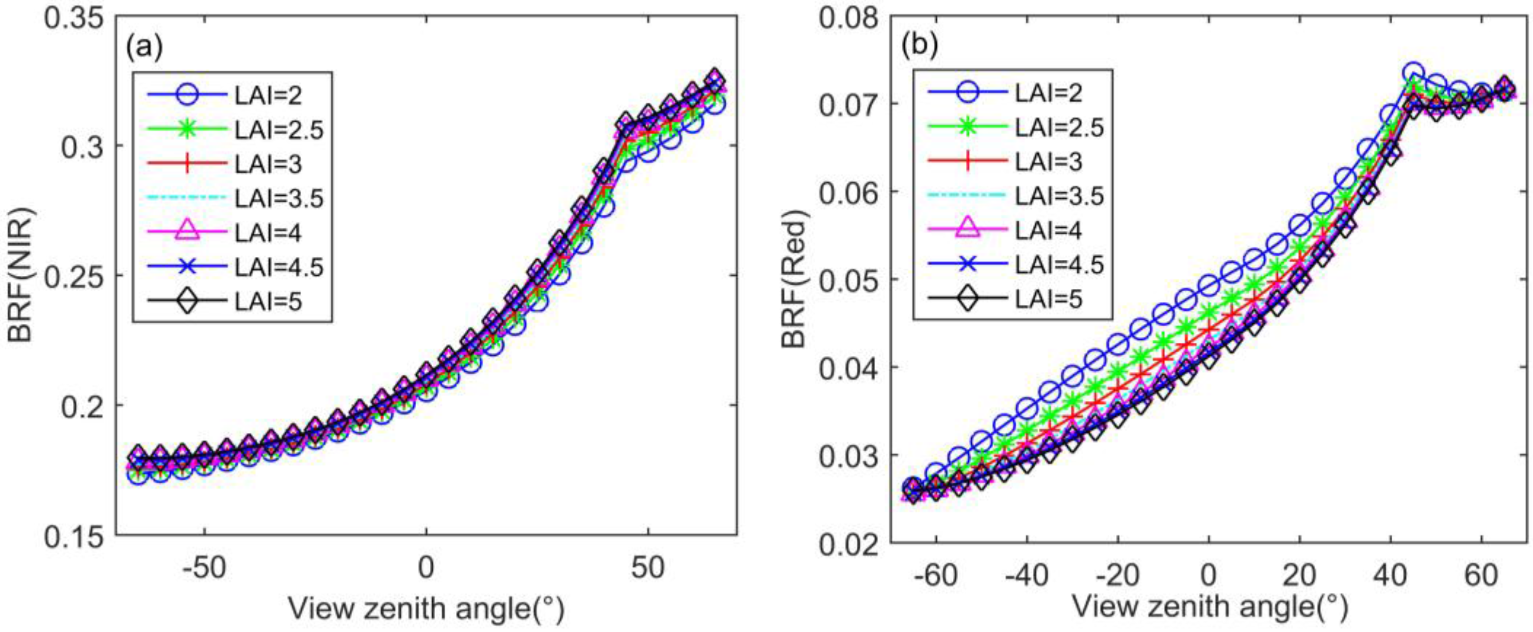
4.1.1. Tendency of the BRF Simulated by MGOMS Model along with the Variation of LAI

The GOMS model can be used to simulate BRF, and the simulation results can accurately reflect the hotspot and bowl-shape effect of the canopy’s BRDF. The MGOMS model derived from the GOMS model must possess the same properties as the GOMS model. When calculating BRF using the MGOMS model, all the input parameters (G, C, Z, LAI, b/R, h/b, $\Delta \text{h}/\text{b}$, ${\theta }_{\text{i}},{Ø}_{\text{i}},{\text{ θ}}_{\text{v}},{Ø}_{\text{v}}$, n, q) are constant as in Table 1, except for LAI, and the influence of the slope and aspect are neglected. In this part, forest canopy reflectance in the principle plane is simulated with gradually increasing LAI in both the red and NIR bands by MGOMS model (Figure 5) (we regard viewing positions near the principal plane on the hotspot side as the “backward observation” and viewing positions near the principal plane opposite the hotspot as the “forward observation”). The results show that BRFs decreased with increasing LAI in the red band and increased with rising LAI in the NIR band. The simulated BRFs reveal the hotspot effect of BRDF in the red and NIR bands and the bowl-shape effect in the NIR band. Additionally, the variation of BRFs with gradually increasing LAI also appropriately reflects the optical characteristics of the vegetation spectral curve.

Figure 5. BRF estimated by MGOMS along with the increased LAI against the view zenith angle in the principal plane with a solar zenith angle of 45° in the (a) NIR band and (b) red band. LAI was gradually increased from 2 to 5 with a data change interval of 0.5. Other parameters in MGOMS were fixed. Negative view zenith angle means the forward observation.

Figure 5. BRF estimated by MGOMS along with the increased LAI against the view zenith angle in the principal plane with a solar zenith angle of 45° in the (a) NIR band and (b) red band. LAI was gradually increased from 2 to 5 with a data change interval of 0.5. Other parameters in MGOMS were fixed. Negative view zenith angle means the forward observation.

The results demonstrate that the MGOMS model is consistent with the GOMS model and can be used to calculate BRFs. Due to the fact that LAI and other canopy structure parameters are not independent in the model, the results only indicate that the MGOMS model has the same characteristics as the GOMS model in the threshold range of the input parameters.

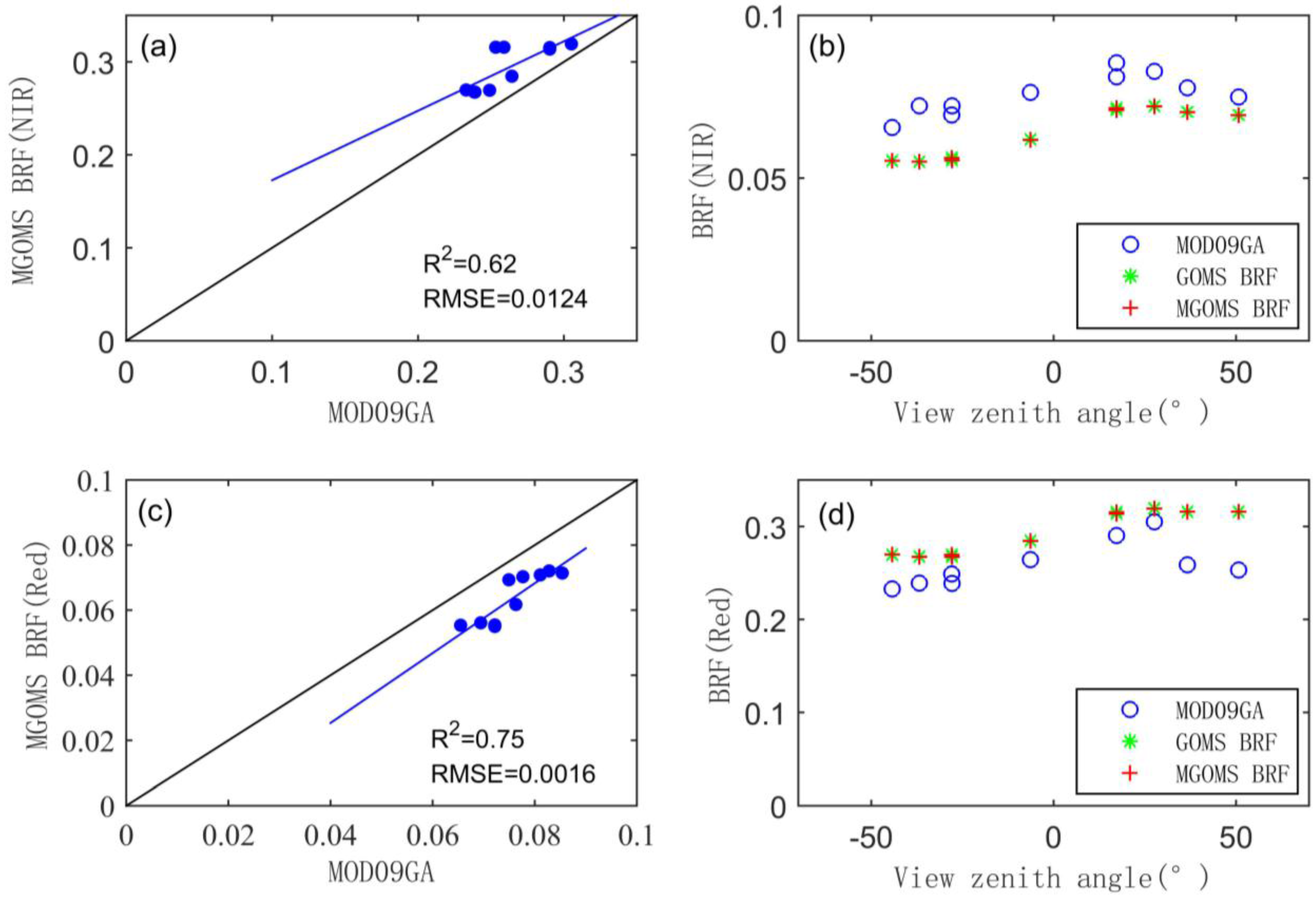
4.1.2. Comparison of the Simulated BRF and MOD09GA BRF

We compared the BRF simulated by the MGOMS model with the MOD09GA BRF products at the 500-m pixel scale (the compared pixels are the pixels where the sample plots located); the solar position, view position, and DOY of the selected MOD09GA BRF data are shown in Figure 3, and the initial data for the model are shown in Table 1.

Figure 6a presents the results of the comparison of the simulated BRF and MOD09GA BRF in the NIR band with an RMSE of 0.0124 and an ${\text{R}}^2$ of 0.62. Figure 6c presents the results of the comparison of the simulated BRF and MOD09GA BRF in the red band with an RMSE of 0.0016 and an ${\text{R}}^2$ of 0.75. Figure 6b,d present the results of the comparison of the simulated BRF and MOD09GA BRF along with the view zenith angle in the NIR and red bands, respectively. The comparison results reveal that the MGOMS model can be used to simulate the BRF precisely (Figure 6a,c). The results presented in Figure 6b,d clearly indicate that the GOMS and MGOMS models have a high consistency in simulating BRF. However, the simulated BRFs were higher than the MOD09GA BRFs in the NIR band and lower than the MOD09GA BRFs in the red band. This is mainly because the simulated BRFs are closely related to the initial values, and the initial values of the model are set according to the field-measured data, which only represent the sample plot of 25 m × 25 m. However, at the 500-m spatial resolution of the MOD09GA BRF products, the unmatched pixel size scale would cause some error; for example, the field-measured LAI of the A sample plots was higher than the LAI of a 500 m × 500 m pixel (the sub-pixel coverage is higher than the pixel coverage of the A sample plot, derived from Section 4.2), which lead to overestimation of the simulated BRFs in the NIR band and underestimation in the red band.

Figure 6. BRF comparison results for simulated BRFs and MOD09GA BRFs. Comparison of the simulated BRF by the MGOMS model and MOD09GA BRF in the (a) NIR band and (c) red band; Comparison of the simulated BRF (simulated by the GOMS and MGOMS models) and MOD09GA BRF along with the view zenith angle in the (b) NIR band and (d) red band. (Negative view zenith angles means the foreward observation).

Figure 6. BRF comparison results for simulated BRFs and MOD09GA BRFs. Comparison of the simulated BRF by the MGOMS model and MOD09GA BRF in the (a) NIR band and (c) red band; Comparison of the simulated BRF (simulated by the GOMS and MGOMS models) and MOD09GA BRF along with the view zenith angle in the (b) NIR band and (d) red band. (Negative view zenith angles means the foreward observation).

4.2. MGOMS Model Application Validation

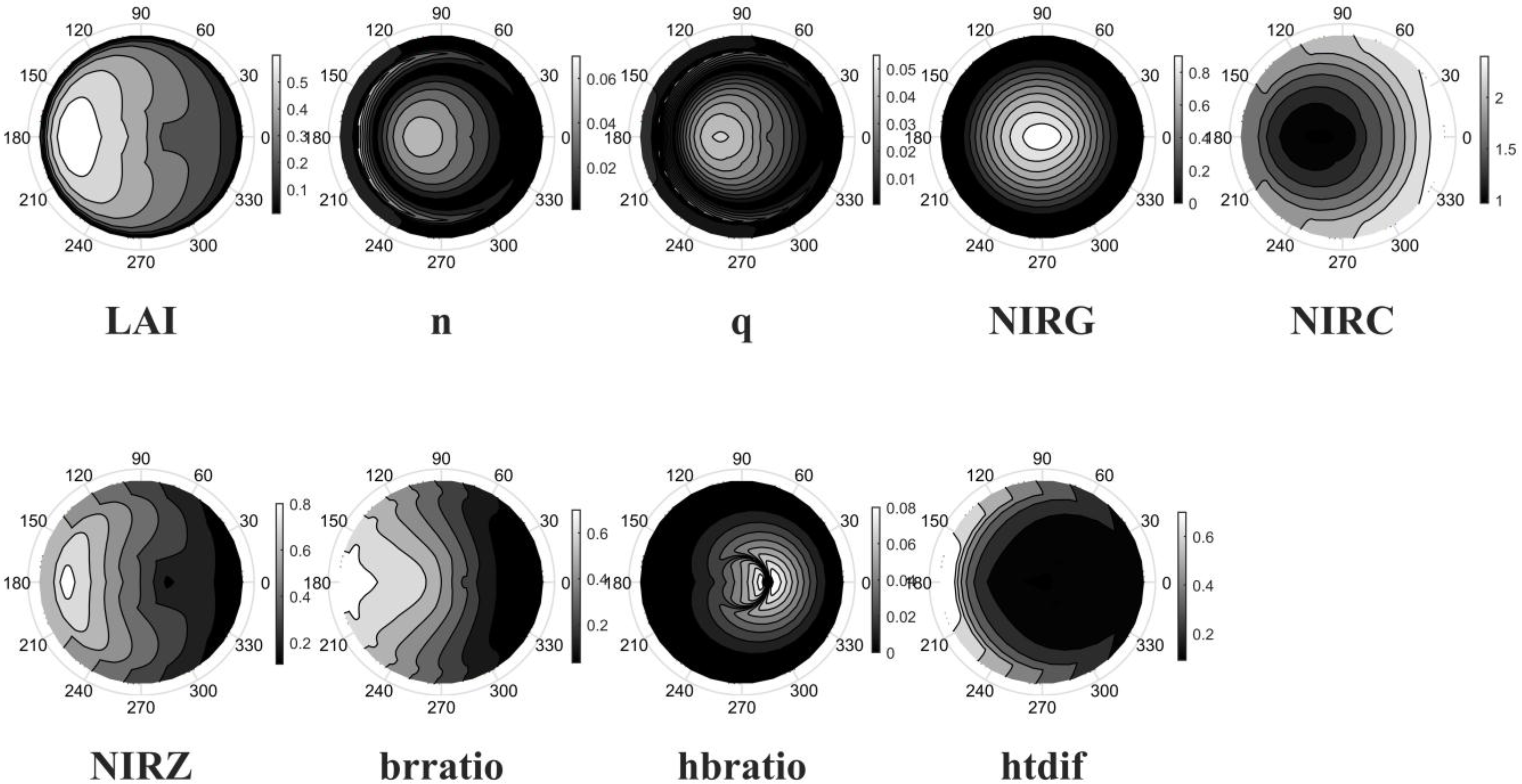
4.2.1. Uncertainty and Sensitivity Analysis of the Parameters in MGOMS Model

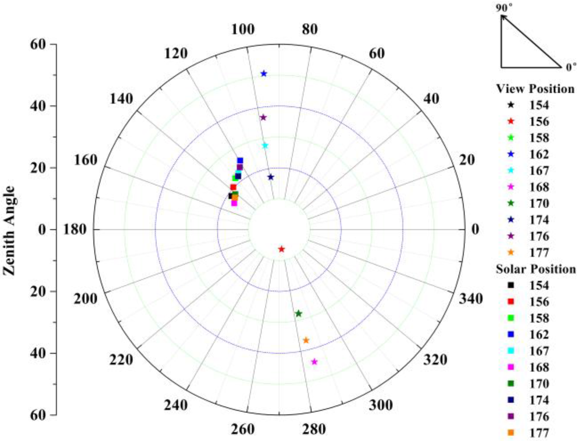
BRFs in the NIR band can well reflect the vegetation coverage features. In our research, BRFs in the NIR band were used to invert LAI. Table 2 presents the first USM matrix (USM0) in the NIR band. The solar zenith angle, solar azimuth, view zenith angle, and view azimuth were derived from the selected MOD09GA data shown in Figure 5. On these days, the solar positions were nearly identical and, thus, we set the solar zenith angle equal to 23° and the solar azimuth equal to 143°. Figure 7 shows the first uncertainty and sensitivity analysis results in the NIR band in all directions, the solar zenith and solar azimuths are 23° and 0°, respectively, in this analysis process. The results indicate that NIRC was the most sensitive parameter, and the USM0 data of NIRC were the highest. The results also demonstrate that the uncertainty of NIRC is more sensitive in the backward observation than in the forward observation. Hence, we first invert NIRC to reduce the uncertainty of the parameter NIRC, and then calculate the average NIRC as the initial value for the second uncertainty and sensitivity analysis to determine the second most sensitive parameter, etc. Based on the results of these analyses, LAI was the third most sensitive parameter and was in the third order in the inversion process. When the sensitivities of the parameters are similar, the parameters are always inverted simultaneously. As our main purpose was to invert LAI, we did not assess whether the sensitivities of the other parameters were similar to that of LAI.

Table 2. The first uncertainty and sensitivity analyses matrix (USM0) results in the NIR band (the solar zenith angle was 23°, and the solar azimuth was 143°). The multi-angles were derived from the MODIS BRF datasets, the DOY of which are shown in Figure 3. (A higher data value indicates a higher sensitivity of the parameter in the model.)

VZA (°)	VAA (°)	NIRG	NIRC	NIRZ	LAI	n	q	b/R	h/b	Δh/b
27.88	282.92	0.81	0.96	0.59	0.58	0.05	0.04	0.59	0.02	0.03
6.39	276.92	0.95	1.00	0.44	0.48	0.05	0.04	0.54	0.04	0.07
17.22	99.05	0.86	1.27	0.31	0.35	0.04	0.03	0.38	0.07	0.14
50.74	95.61	0.50	1.64	0.28	0.33	0.00	−0.01	0.25	0.04	0.12
27.58	99.47	0.72	1.44	0.29	0.33	0.03	0.03	0.31	0.07	0.17
44.27	284.89	0.58	1.08	0.70	0.63	0.04	0.03	0.61	0.01	0.08
36.65	98.06	0.59	1.56	0.31	0.34	0.03	0.02	0.25	0.06	0.14
36.86	283.61	0.70	1.02	0.65	0.61	0.05	0.04	0.60	0.01	0.06

Table 2. The first uncertainty and sensitivity analyses matrix (USM0) results in the NIR band (the solar zenith angle was 23°, and the solar azimuth was 143°). The multi-angles were derived from the MODIS BRF datasets, the DOY of which are shown in Figure 3. (A higher data value indicates a higher sensitivity of the parameter in the model.)

VZA (°)	VAA (°)	NIRG	NIRC	NIRZ	LAI	n	q	b/R	h/b	Δh/b
27.88	282.92	0.81	0.96	0.59	0.58	0.05	0.04	0.59	0.02	0.03
6.39	276.92	0.95	1.00	0.44	0.48	0.05	0.04	0.54	0.04	0.07
17.22	99.05	0.86	1.27	0.31	0.35	0.04	0.03	0.38	0.07	0.14
50.74	95.61	0.50	1.64	0.28	0.33	0.00	−0.01	0.25	0.04	0.12
27.58	99.47	0.72	1.44	0.29	0.33	0.03	0.03	0.31	0.07	0.17
44.27	284.89	0.58	1.08	0.70	0.63	0.04	0.03	0.61	0.01	0.08
36.65	98.06	0.59	1.56	0.31	0.34	0.03	0.02	0.25	0.06	0.14
36.86	283.61	0.70	1.02	0.65	0.61	0.05	0.04	0.60	0.01	0.06

According to the sensitivity analysis results, the steps for inversion and segmentation of the BRF data were as follows:

(1)

Invert NIRC using the NIR band reflectance datasets with backward-viewing directions and large viewing zenith angles;

(2)

Invert NIRG using the NIR band reflectance datasets with small viewing zenith angles;

(3)

Invert LAI (LAIJune) using the reflectance datasets for June with forward-viewing directions and large viewing zenith angles.

Figure 7. Polar coordinate graph of the first uncertainty and sensitivity analyses matrix results in the NIR band in all view directions. The solar zenith and solar azimuth were 23° and 0°, respectively. The data values have no unit. A higher data value indicates a higher sensitivity of the parameter in the model.

Figure 7. Polar coordinate graph of the first uncertainty and sensitivity analyses matrix results in the NIR band in all view directions. The solar zenith and solar azimuth were 23° and 0°, respectively. The data values have no unit. A higher data value indicates a higher sensitivity of the parameter in the model.

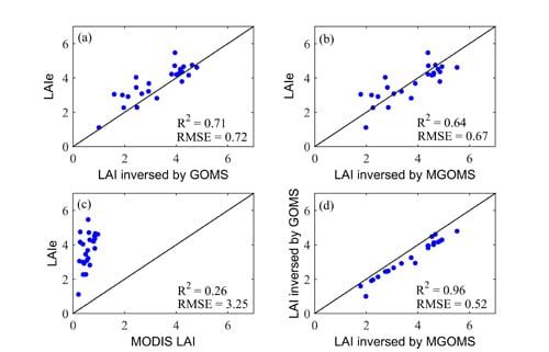
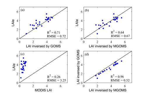
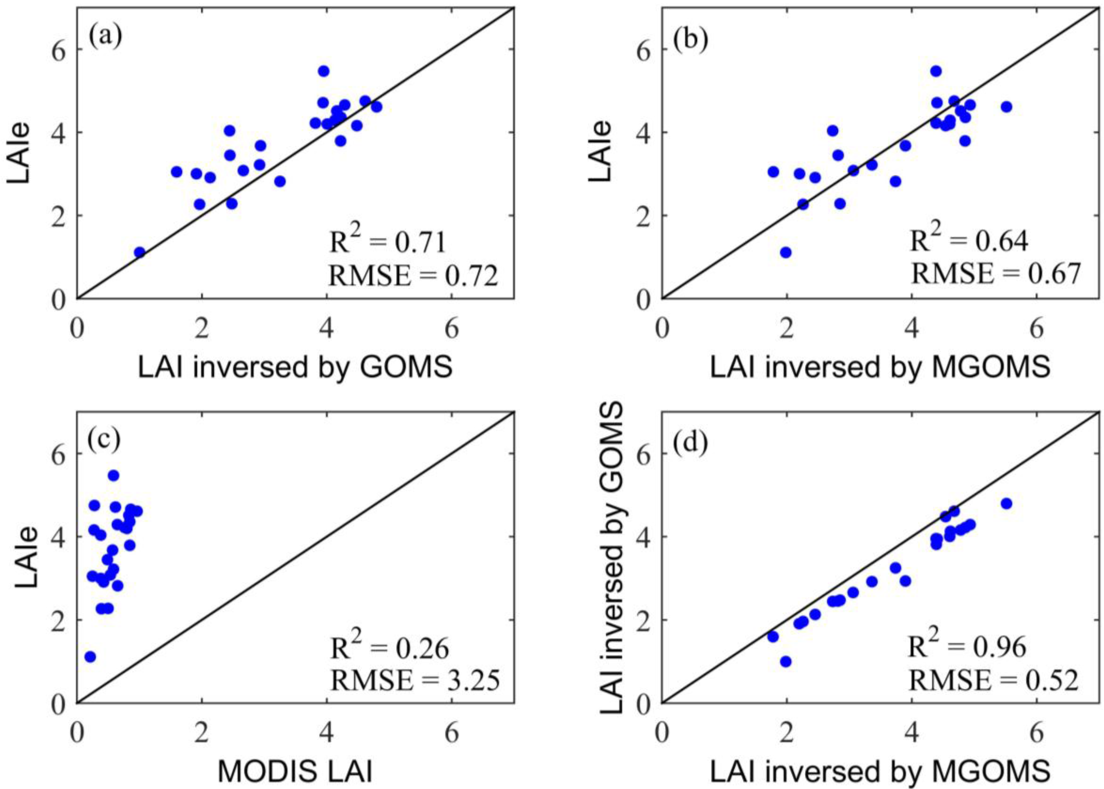
4.2.2. LAI Inversion Based on Retrieved Parameters by MGOMS Model

The results of the parameter uncertainty and sensitivity analysis indicated that LAI was the third most sensitive parameter in the NIR band of the MGOMS model. Thus, we first inverted NIRC, then used the inversion results as the prior knowledge to invert NIRG, and finally obtained the inversion results of LAI. Compared with the GOMS model, the MGOMS model can effectively abridge the LAI inversion process. The input parameters were described in Section 3.3.1.

Figure 8 shows the LAI inversion results for June 2008 obtained using the MGOMS model; the pixel scale is 500 m with 300 × 380 pixels. Considering the real surface condition in the Dayekou forest, the density of the trees decreases and the shape of the tree canopy becomes smaller with increasing altitude, indicating that LAI will decrease with increasing altitude. From the DEM map of Dayekou shown in Figure 1b, the altitude increases with decreasing latitude and longitude. Therefore, in Dayekou forest, the LAI should show a decrease with decreasing latitude and longitude. As shown in Figure 8, LAI decreases with decreasing latitude and longitude on the whole. The change of the retrieved LAI with decreasing latitude and longitude is approximately in agreement with the real condition in Dayekou forest. This result shows that the MGOMS model can be used to invert LAI in large areas.

4.2.3. Precision of the Retrieved LAI by MGOMS Model

In order to validate the LAI inversion efficiency of the MGOMS model, the retrieved LAI was compared with the field-measured LAI in situ. As described in Section 2.2.1, the forest LAI was measured using LAI-2000 and TRAC in the A (20 m × 20 m) and B (25 m × 25 m) sample plots. The retrieved LAI must be adjusted to the in situ scale to enable a robust validation. The ${\text{LAI}}_{\text{e}}$ at different scales (subpixel and pixel) has the relationship shown below [36]

$$\frac{{\text{LAI}}_{\text{subpixel}}}{{\text{LAI}}_{\text{pixel}}}=\frac{{\left({\text{b * nR}}^2\right)}_{\text{subpixel}}}{{\left({\text{b * nR}}^2\right)}_{\text{pixel}}}$$

(24)

where ${\text{LAI}}_{\text{subpixel}}$ is the field-measured LAI and ${\text{LAI}}_{\text{pixel}}$ is the retrieved LAI. The parameters on the right side can be obtained from the LiDAR image. b can be calculated from H. H can be derived from the LiDAR data (CHM), and the statistical relationship between b and H can be built using field-measured b and H. ${\text{nR}}^2$ is considered to be approximately equal to the canopy cover factor, which can be calculated as the ratio between the number of canopy pixels and the number of corresponding CHM pixels classified with a zero threshold.

Figure 8. LAI inversion results of Dayekou forest in June 2008. The retrieved LAI data value is 0 to 6. The size of the map is identical to that in Figure 1a. The pixels in the inversion process are only the forest pixels, and the others are set to zero and colored white in this map.

Figure 8. LAI inversion results of Dayekou forest in June 2008. The retrieved LAI data value is 0 to 6. The size of the map is identical to that in Figure 1a. The pixels in the inversion process are only the forest pixels, and the others are set to zero and colored white in this map.

Due to the sample plots A5-9 not being forest pixels in the MODIS land-cover product, there were only 24 field-measured ${\text{LAI}}_{\text{e}}$ validation data points in this part. We also compared the LAI retrieved by Ma et al. [36], i.e., LAI retrieved by the GOMS model (which cannot be directly inverted by the GOMS model, by using the structure parameter retrieved by the GOMS model and other statistical relationships to calculate LAI), with the LAI retrieved by the MGOMS model. Figure 9 shows the validation results.

Figure 9a–c show the effective LAI measured by LAI-2000 and TRAC versus LAI retrieved by the GOMS model, LAI retrieved by the MGOMS model and MODIS LAI, respectively. Figure 9d shows the results of the comparison of ${\text{LAI}}_{\text{e}}$ retrieved by the GOMS model and ${\text{LAI}}_{\text{e}}$ retrieved by the MGOMS model. Both the GOMS and MGOMS models can achieve high accuracy in calculating LAI and were in good agreement with the field-measured LAI, with ${\text{R}}^2$ of 0.71 and 0.64, respectively. However, MODIS LAI produced much lower ${\text{R}}^2$ values compared with the field-measured LAI (Figure 9d). The RMSE value between the field-measured LAI and the MODIS LAI (3.25) is much higher than that between the field-measured LAI and the GOMS and MGOMS LAI (0.71 and 0.67). Figure 9d compares the ${\text{LAI}}_{\text{e}}$ retrieved by the MGOMS model and the ${\text{LAI}}_{\text{e}}$ retrieved by the GOMS model. The high ${\text{R}}^2$ (0.96) and low RMSE (0.5243) indicate that the MGOMS model was very consistent with the GOMS model, combined with other statistical relationships, for calculating LAI. The ${\text{LAI}}_{\text{e}}$ retrieved by the MGOMS model was higher than the ${\text{LAI}}_{\text{e}}$ calculated by the GOMS model, but the ${\text{LAI}}_{\text{e}}$ retrieved by the MGOMS model was closer to the field-measured ${\text{LAI}}_{\text{e}}$, with a lower RMSE (0.67).

Figure 9. Comparison between the retrieved LAI and field-measured model LAI_e of the sample plots: (a) LAI_e retrieved by the GOMS model compared with field-measured LAI_e with R² of 0.71 and RMSE of 0.72; (b) ${\text{LAI}}_{\text{e}}$ retrieved by the MGOMS model compared with field-measured ${\text{LAI}}_{\text{e}}$, with ${\text{R}}^2$ of 0.64 and RMSE of 0.67; (c) MODIS LAI compared with field-measured ${\text{LAI}}_{\text{e}}$, with ${\text{R}}^2$ of 0.26 and RMSE of 3.25; (d) ${\text{LAI}}_{\text{e}}$ retrieved by the MGOMS model compared with ${\text{LAI}}_{\text{e}}$ retrieved by the GOMS model, with ${\text{R}}^2$ of 0.96 and RMSE of 0.52.

Figure 9. Comparison between the retrieved LAI and field-measured model LAI_e of the sample plots: (a) LAI_e retrieved by the GOMS model compared with field-measured LAI_e with R² of 0.71 and RMSE of 0.72; (b) ${\text{LAI}}_{\text{e}}$ retrieved by the MGOMS model compared with field-measured ${\text{LAI}}_{\text{e}}$, with ${\text{R}}^2$ of 0.64 and RMSE of 0.67; (c) MODIS LAI compared with field-measured ${\text{LAI}}_{\text{e}}$, with ${\text{R}}^2$ of 0.26 and RMSE of 3.25; (d) ${\text{LAI}}_{\text{e}}$ retrieved by the MGOMS model compared with ${\text{LAI}}_{\text{e}}$ retrieved by the GOMS model, with ${\text{R}}^2$ of 0.96 and RMSE of 0.52.

5. Discussions

The MGOMS model, which is derived from the GOMS model, has the same characteristics in modeling BRF as the GOMS model. In Figure 6a,c, the results suggest that the BRF simulated by MGOMS model is closely related to the MODIS BRF data. In the NIR band, the ${\text{R}}^2$ and RMSE are 0.62 and 0.0124, respectively, and in the red band, the R² and RMSE are 0.75 and 0.0016. The relatively high R² and low RMSE indicate that the MGOMS model can be used to simulate BRF. In Figure 6b,d, it is clear that the BRF datasets simulated by the GOMS and MGOMS models are nearly equivalent when the field-measured data are used as the initial value. This result further demonstrates that MGOMS model is consistent with GOMS model.

The GOMS model is the most widely-used physical model to invert LAI because the model builds the canopy structure parameters and BRF together. With the multi-angle BRF datasets, such as the MODIS and MISR datasets, it is easy to build the invert function and retrieve all parameters belonging to the GOMS model. The MGOMS model is derived from the GOMS model and, thus, shares this advantage. Previous studies [36,37] of LAI inversion using the GOMS model have inverted the canopy structure parameters (e.g., b/R, h/b, nR²) first and then used the statistical model to calculate LAI. By contrast, the MGOMS model can retrieve LAI directly. The USM results indicated that LAI is in the third order of the MSDT inversion process, and using the MGOMS model abridges the LAI inversion process.

Compared with the field-measured LAI, the LAI_e values retrieved by both the MGOMS and GOMS models are in good agreement with the field-measured LAI, with R² of 0.64 and 0.71, respectively. Although the R² of LAI_e retrieved by the MGOMS model is slightly lower than that of LAI_e retrieved by the GOMS model, the RMSE of LAI_e retrieved by MGOMS (0.67) is lower than that of LAI_e retrieved by GOMS (0.72). These results all demonstrate that the MGOMS model can be used to invert LAI.

However, the GOMS model was constructed based on the Li-Strahler geometric-optical model, which considers the mutual shadowing of crowns and makes the geometric optic model more suitable for highly-dense canopy forests. However, in our modified process, when considering the mutual shadowing of crowns, the P(s|n) function is difficult to build, and the P_gap function will be very complex. In order to make the function between LAI and nR² laconic, we assumed that the crowns are non-overlapping and that the crowns in the field of view are uniformly distributed. Based on this assumption, the MGOMS model may be less precise than the GOMS model in dense forest, with a smaller applicable scope than the GOMS model. Thus, further research must address the development of the LAI and nR² relationship function when the crowns are non-overlapping and the crowns are Poisson-distributed.

6. Conclusions

In this study, the GOMS model was modified by using LAI to replace nR². The modified GOMS (MGOMS) model enabled the direct inversion of LAI, and LAI is a relatively highly-sensitive parameter in the MGOMS model. By using the MGOMS model, the LAI inversion process was effectively reduced. When comparing the retrieved LAIe with the field-measured LAIe , though the LAI retrieved by the MGOMS model had a slightly lower R² (0.64) than the LAI retrieved by the GOMS model (0.71), the LAI retrieved by the MGOMS model was closer to the field-measured LAI (with an RMSE of 0.67) than the LAI retrieved by the GOMS model (with an RMSE of 0.72). All of these results indicate that the MGOMS model can be used to invert LAI effectively and precisely. However, many problems remain to be addressed in the future, such as, in the modeling process, we make the assumption that the canopies are non-overlapping and uniformly distributed. We also assume that the view zenith angle is zero. Moreover, we set the parameter G to a constant value of 0.5. All of these assumptions can affect the accuracy of the model. In addition, the precision of the prior information also influences the calculated results of the MGOMS model. Therefore, in a forthcoming study, we will focus on how to expand the applicability of the MGOMS model and how to solve the uncertainty of the input parameters.

References

1. Chen, J.M.; Black, T. Defining leaf area index for non-flat leaves. Plant Cell Environ. 1992, 15, 421–429. [Google Scholar] [CrossRef]
2. Che, M.L.; Chen, B.Z.; Zhang, H.F.; Fang, S.F.; Xu, G.; Lin, X.F.; Wang, Y.C. A new equation for deriving vegetation phenophase from time series of leaf area index (LAI) data. Remote Sens. 2014, 6, 5650–5670. [Google Scholar] [CrossRef]
3. Zhao, B.; Yao, X.; Tian, Y.C.; Liu, X.J.; Ata-Ul-Karim, S.T.; Ni, J.; Cao, W.X.; Zhu, Y. New critical nitrogen curve based on leaf area index for winter wheat. Agron. J. 2014, 106, 379–389. [Google Scholar] [CrossRef]
4. Aboelghar, M.; Ali, A.R.; Arafat, S. Spectral wheat yield prediction modeling using spot satellite imagery and leaf area index. Arabian J. Geosci. 2014, 7, 465–474. [Google Scholar] [CrossRef]
5. Qu, Y.H.; Zhu, Y.Q.; Han, W.C.; Wang, J.D.; Ma, M.G. Crop leaf area index observations with a wireless sensor network and its potential for validating remote sensing products. IEEE J. Sel. Top. Appl. Earth Observ. Remote Sens. 2014, 7, 431–444. [Google Scholar] [CrossRef]
6. Wang, H.; Zhu, Y.; Li, W.L.; Cao, W.X.; Tian, Y.C. Integrating remotely sensed leaf area index and leaf nitrogen accumulation with ricegrow model based on particle swarm optimization algorithm for rice grain yield assessment. J. Appl. Remote Sens. 2014, 8. [Google Scholar] [CrossRef]
7. Bal, S.K.; Choudhury, B.U.; Sood, A.; Saha, S.; Mukherjee, J.; Singh, H.; Kaur, P. Relationship between leaf area index of wheat crop and different spectral indices in punjab. J. Agrometeorol. 2013, 15, 98–102. [Google Scholar]
8. Biudes, M.S.; Machado, N.G.; Danelichen, V.H.D.; Souza, M.C.; Vourlitis, G.L.; Nogueira, J.D. Ground and remote sensing-based measurements of leaf area index in a transitional forest and seasonal flooded forest in Brazil. Int. J. Biometeorol. 2014, 58, 1181–1193. [Google Scholar] [CrossRef] [PubMed]
9. Taugourdeau, S.; le Maire, G.; Avelino, J.; Jones, J.R.; Ramirez, L.G.; Quesada, M.J.; Charbonnier, F.; Gomez-Delgado, F.; Harmand, J.M.; Rapidel, B.; et al. Leaf area index as an indicator of ecosystem services and management practices: An application for coffee agroforestry. Agric. Ecosyst. Environ. 2014, 192, 19–37. [Google Scholar] [CrossRef]
10. Tesemma, Z.K.; Wei, Y.P.; Western, A.W.; Peel, M.C. Leaf area index variation for crop, pasture, and tree in response to climatic variation in the goulburn-broken catchment, australia. J. Hydrometeorol. 2014, 15, 1592–1606. [Google Scholar] [CrossRef]
11. Zhang, H.K.; Chen, J.M.; Huang, B.; Song, H.H.; Li, Y.R. Reconstructing seasonal variation of landsat vegetation index related to leaf area index by fusing with modis data. IEEE J. Sel. Top. Appl. Earth Observ. Remote Sens. 2014, 7, 950–960. [Google Scholar] [CrossRef]
12. Leonenko, G.; Los, S.O.; North, P.R.J. Retrieval of leaf area index from modis surface reflectance by model inversion using different minimization criteria. Remote Sens. Environ. 2013, 139, 257–270. [Google Scholar] [CrossRef]
13. Le Maire, G.; Marsden, C.; Nouvellon, Y.; Stape, J.L.; Ponzoni, F.J. Calibration of a species-specific spectral vegetation index for leaf area index (LAI) monitoring: Example with modis reflectance time-series on eucalyptus plantations. Remote Sens. 2012, 4, 3766–3780. [Google Scholar] [CrossRef] [Green Version]
14. Luo, S.Z.; Wang, C.; Zhang, G.B.; Xi, X.H.; Li, G.C. Forest leaf area index (LAI) inversion using airborne lidar data. Chin. J. Geophys. Chin. Ed. 2013, 56, 1467–1475. [Google Scholar]
15. Manninen, T.; Stenberg, P.; Rautiainen, M.; Voipio, P. Leaf area index estimation of boreal and subarctic forests using vv/hh envisat/asar data of various swaths. IEEE Trans. Geosci. Remote Sens. 2013, 51, 3899–3909. [Google Scholar] [CrossRef]
16. Liu, C.W.; Kang, S.Z.; Li, F.S.; Li, S.; Du, T.S. Canopy leaf area index for apple tree using hemispherical photography in arid region. Sci. Hortic. 2013, 164, 610–615. [Google Scholar] [CrossRef]
17. Leblanc, S.G.; Fournier, R.A. Hemispherical photography simulations with an architectural model to assess retrieval of leaf area index. Agric. For. Meteorol. 2014, 194, 64–76. [Google Scholar] [CrossRef]
18. Kumar, V.; Kumari, M.; Saha, S.K. Leaf area index estimation of lowland rice using semi-empirical backscattering model. J. Appl. Remote Sens. 2013, 7. [Google Scholar] [CrossRef]
19. Gonsamo, A.; Chen, J.M. Continuous observation of leaf area index at fluxnet-canada sites. Agric. For. Meteorol. 2014, 189, 168–174. [Google Scholar] [CrossRef]
20. Suits, G.H. The calculation of the directional reflectance of a vegetative canopy. Remote Sens. Environ. 1971, 2, 117–125. [Google Scholar] [CrossRef]
21. Suits, G.H. The cause of azimuthal variations in directional reflectance of vegetative canopies. Remote Sens. Environ. 1971, 2, 175–182. [Google Scholar] [CrossRef]
22. Verhoef, W. Light scattering by leaf layers with application to canopy reflectance modeling: The sail model. Remote Sens. Environ. 1984, 16, 125–141. [Google Scholar] [CrossRef]
23. Reyna, E.; Badhwar, G.D. Inclusion of specular reflectance in vegetative canopy models. IEEE Trans. Geosci. Remote Sens. 1985, GE-23, 731–736. [Google Scholar] [CrossRef]
24. Jackson, R.D.; Reginato, R.J.; Pinter, J.P.J.; Idso, S.B. Plant canopy information extraction from composite scene reflectance of row crops. Appl. Opt. 1979, 18, 3775–3782. [Google Scholar] [PubMed]
25. Norman, J.M.; Welles, J.M.; Walter, E.A. Contrasts among bidirectional reflectance of leaves, canopies, and soils. IEEE Trans. Geosci. Remote Sens. 1985, GE-23, 659–667. [Google Scholar] [CrossRef]
26. Ross, J. Radiative transfer in plant communities. Veg. Atmos. 1975, 1, 13–55. [Google Scholar]
27. Li, X.; Strahler, A.H. Geometric-optical bidirectional reflectance modeling of a conifer forest canopy. IEEE Trans. Geosci. Remote Sens. 1986, GE-24, 906–919. [Google Scholar] [CrossRef]
28. Li, X.; Strahler, A.H. Geometric-optical modeling of a conifer forest canopy. IEEE Trans. Geosci. Remote Sens. 1985, GE-23, 705–721. [Google Scholar] [CrossRef]
29. Schaaf, C.B.; Li, X.; Strahler, A.H. Topographic effects on bidirectional and hemispherical reflectances calculated with a geometric-optical canopy model. IEEE Trans. Geosci. Remote Sens. 1994, 32, 1186–1193. [Google Scholar] [CrossRef]
30. Qi, J.; Kerr, Y.H.; Moran, M.S.; Weltz, M.; Huete, A.R.; Sorooshian, S.; Bryant, R. Leaf area index estimates using remotely sensed data and brdf models in a semiarid region. Remote Sens. Environ. 2000, 73, 18–30. [Google Scholar] [CrossRef]
31. Li, X.; Strahler, A.H. Geometric-optical bidirectional reflectance modeling of the discrete crown vegetation canopy: Effect of crown shape and mutual shadowing. IEEE Trans. Geosci. Remote Sens. 1992, 30, 276–292. [Google Scholar] [CrossRef]
32. Strahler, A.H.; Jupp, D.L.B. Modeling bidirectional reflectance of forests and woodlands using boolean models and geometric optics. Remote Sens. Environ 1990, 34, 153–166. [Google Scholar] [CrossRef]
33. Li, X.; Wang, J.; Strahler, A.H. A hybrid geometric optical-radiative transfer approach for modeling light absorption and albedo of discontinuous canopies. Sci. China (series B) 1994, 24, 828–836. [Google Scholar]
34. Li, X.; Strahler, A.H.; Woodcock, C.E. A hybrid geometric optical-radiative transfer approach for modeling albedo and directional reflectance of discontinuous canopies. IEEE Trans. Geosci. Remote Sens. 1995, 33, 466–480. [Google Scholar]
35. Li, X.; Strahler, A.H.; Friedl, M.A. A conceptual model for effective directional emissivity from nonisothermal surfaces. IEEE Trans. Geosci. Remote Sens. 1999, 37, 2508–2517. [Google Scholar]
36. Ma, H.; Song, J.; Wang, J.; Xiao, Z.; Fu, Z. Improvement of spatially continuous forest LAI retrieval by integration of discrete airborne lidar and remote sensing multi-angle optical data. Agric. For. Meteorol. 2014, 189, 60–70. [Google Scholar] [CrossRef]
37. Fu, Z.; Wang, J.; Song, J.L.; Zhou, H.M.; Pang, Y.; Chen, B.S. Estimation of forest canopy leaf area index using MODIS, MISR, and LiDAR observations. J. Appl. Remote Sens. 2011, 5. [Google Scholar] [CrossRef]
38. Li, Z.; Xu, Z. Detection of change points in temperature and precipitation time series in the heihe river basin over the past 50 years. Resour. Sci. 2011, 33, 1877–1882. [Google Scholar]
39. Li, X.; Cheng, G.; Liu, S.; Xiao, Q.; Ma, M.; Jin, R.; Che, T.; Liu, Q.; Wang, W.; Qi, Y. Heihe watershed allied telemetry experimental research (hiwater) scientific objectives and experimental design (ei). Bull. Am. Meteorol. Soc. 2013, 94, 1145–1160. [Google Scholar] [CrossRef]
40. Chen, J.M.; Cihlar, J. Plant canopy gap-size analysis theory for improving optical measurements of leaf-area index. Appl. Opt. 1995, 34, 6211–6222. [Google Scholar] [CrossRef] [PubMed]
41. Gower, S.T.; Kucharik, C.J.; Norman, J.M. Direct and indirect estimation of leaf area index, f apar, and net primary production of terrestrial ecosystems. Remote Sens. Environ. 1999, 70, 29–51. [Google Scholar] [CrossRef]
42. Chen, J.M. Optically-based methods for measuring seasonal variation of leaf area index in boreal conifer stands. Agric. For. Meteorol. 1996, 80, 135–163. [Google Scholar] [CrossRef]
43. Zhang, X.; Ma, C.; Hu, H.; Li, F. Radiometric correction based on multi-temporal spot satellite images. In Proceedings of the International Conference on Wireless Communications & Signal Processing, 2009. WCSP 2009, Nanjing, China, 13–15 November 2009; pp. 1–6.
44. Chopping, M.; Moisen, G.G.; Su, L.; Laliberte, A.; Rango, A.; Martonchik, J.V.; Peters, D.P.C. Large area mapping of southwestern forest crown cover, canopy height, and biomass using the nasa multiangle imaging spectro-radiometer. Remote Sens. Environ. 2008, 112, 2051–2063. [Google Scholar] [CrossRef]
45. Li, X.; Strahler, A.H. Modeling the gap probability of a discontinuous vegetation canopy. IEEE Trans. Geosci. Remote Sens. 1988, 26, 161–170. [Google Scholar] [CrossRef]
46. Zhu, Q.J.; Fan, S.H.; Liu, L.F.; Li, X.; Liu, Y. A model of the forest gap probability and its validation. Remote Sens. Environ. China. 1995, 10, 70–75. [Google Scholar]
47. Nilson, T. A theoretical analysis of the frequency of gaps in plant stands. Agric. Meteorol. 1971, 8, 25–38. [Google Scholar] [CrossRef]
48. Wilson, J.W. Stand structure and light penetration. I. Analysis by point quadrats. J. Appl. Ecol. 1965. [Google Scholar] [CrossRef]
49. Miller, J. A formula for average foliage density. Aust. J. Bot. 1967, 15, 141–144. [Google Scholar] [CrossRef]
50. Li, X.; Gao, F.; Wang, J.; Zhu, Q. Uncertainty and sensitivity matrix of parameters in inversion of physical brdf model. J. Remote Sens. 1997, 1, 5–14. [Google Scholar]
51. Tarantola, A. Inverse Problem Theory and Methods for Model Parameter Estimation; SIAM (Society for Industrial and Applied Mathematics): Philadelphia, PA, USA, 2005. [Google Scholar]
52. Boggs, P.T.; Tolle, J.W. Sequential quadratic programming. Acta Numer. 1995, 4, 1–51. [Google Scholar] [CrossRef]
53. Björkman, G. Sequential quadratic programming for non-linear elastic contact problems. Int. J. Numer. Methods Eng. 1995, 38, 137–165. [Google Scholar]