
Remote Sensing-Based Assessment of the Variability of Winter and Summer Precipitation in the Pamirs and Their Effects on Hydrology and Hazards Using Harmonic Time Series Analysis


Abstract
:
1. Introduction
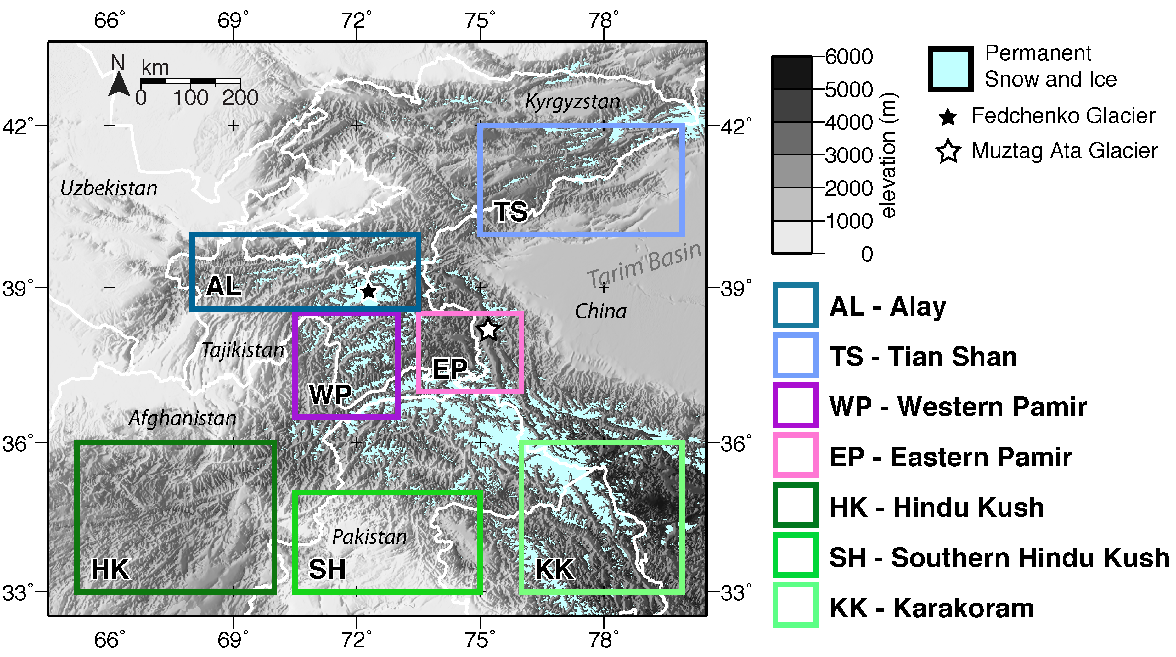
2. Study Area

3. Data

| Country | Event Type | Date | People Affected |
|---|---|---|---|
| 2005 | |||
| AF | Storm | January 2005 | 22,656 |
| AF | Flood | 05 March 2005 | 11003 |
| AF | Flood | 16 June 2005 | 5040 |
| PK | Flood | 09 February 2005 | 7,000,450 |
| PK | Flood | 21 June 2005 | 460,073 |
| PK | Flood | 05 July 2005 | 58,020 |
| PK | Flood | 02 March 2005 | 5000 |
| PK | Flood | 20 March 2005 | 3500 |
| TJ | Flood | 08 June 2005 | 3222 |
| TJ | Mass movement wet | 03 February 2005 | 1953 |
| TJ | Flood | 23 July 2005 | 1890 |
| KY | Flood | 10 June 2005 | 2050 |
| UZ | Flood | 24 February 2005 | 1500 |
| 2008 | |||
| AF | Drought | October 2008 | 280,000 |
| AF | Flood | August 2008 | 1180 |
| PK | Flood | 02 August 2008 | 200,012 |
| PK | Flood | 09 August 2008 | 90,752 |
| TJ | Drought | October 2008 | 800,000 |
| 2010 | |||
| AF | Flood | 05 May 2010 | 40,000 |
| AF | Flood | 27 July 2010 | 5000 |
| PK | Flood | 28 July 2010 | 20,359,496 |
| PK | Mass Movement Wet | 04 January 2010 | 26,700 |
| PK | Storm | 06 June 2010 | 4000 |
| PK | Flood | 21 July 2010 | 4000 |
| PK | Mass Movement Wet | 18 February 2010 | 3705 |
| TJ | Flood | 06 May 2010 | 6708 |
| TJ | Flood | 11 April 2010 | 1914 |
| KY | Mass Movement Wet | 03 June 2010 | 8350 |
4. Methods
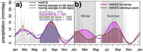
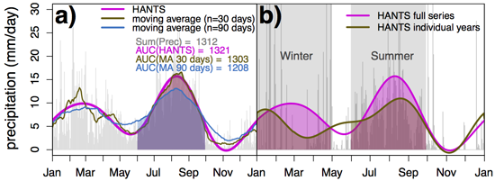
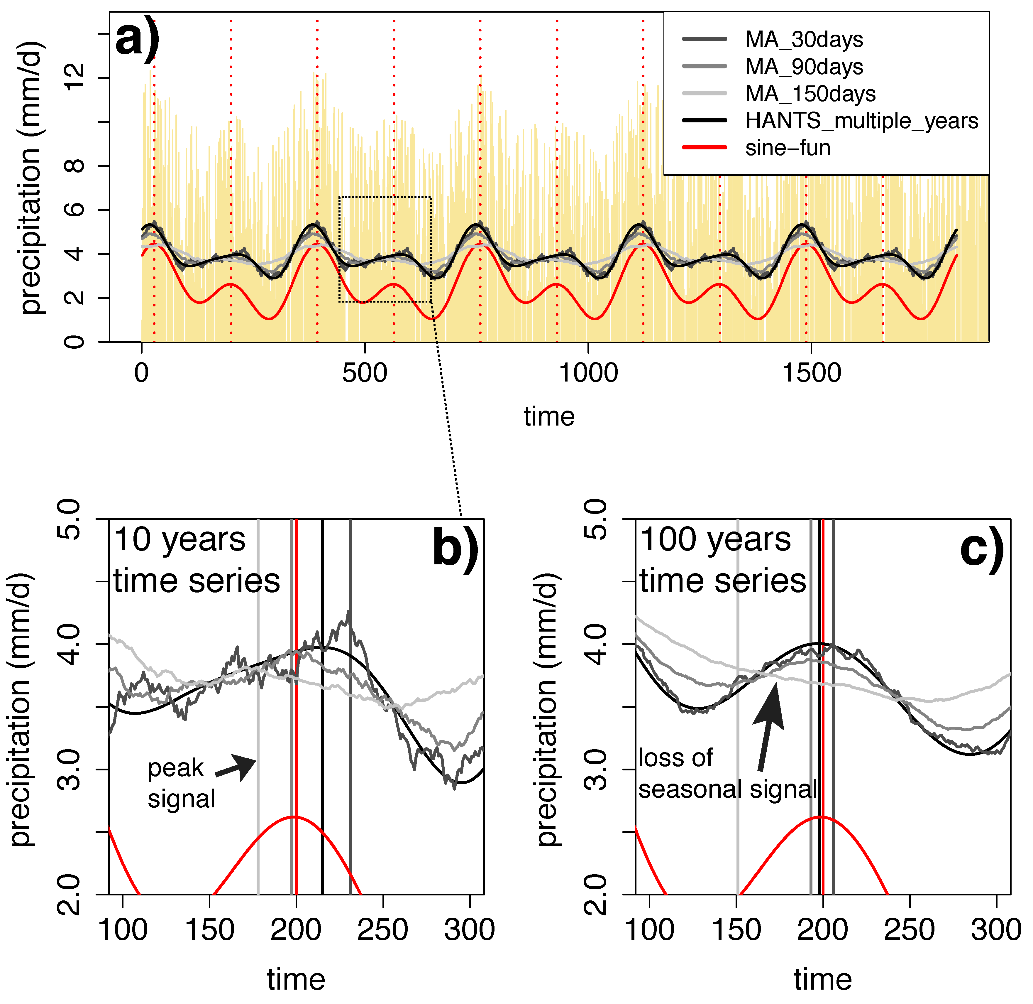
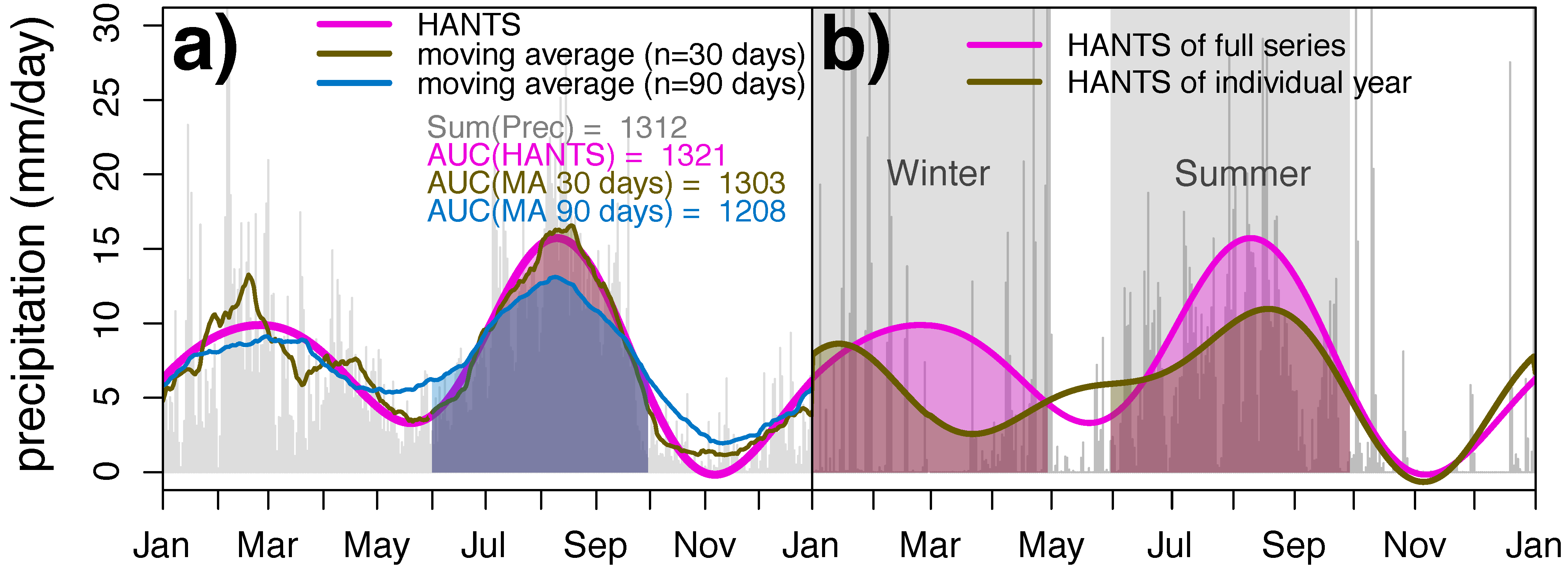
4.1. HANTS

5. Results
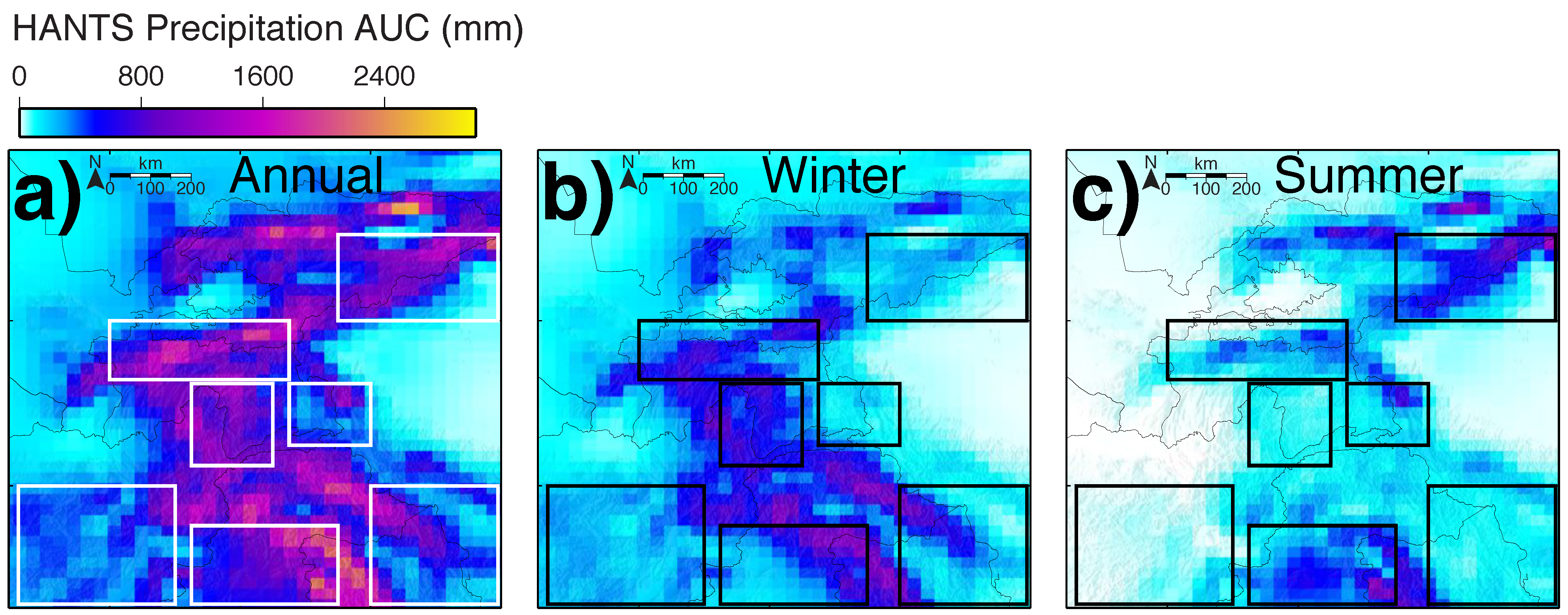
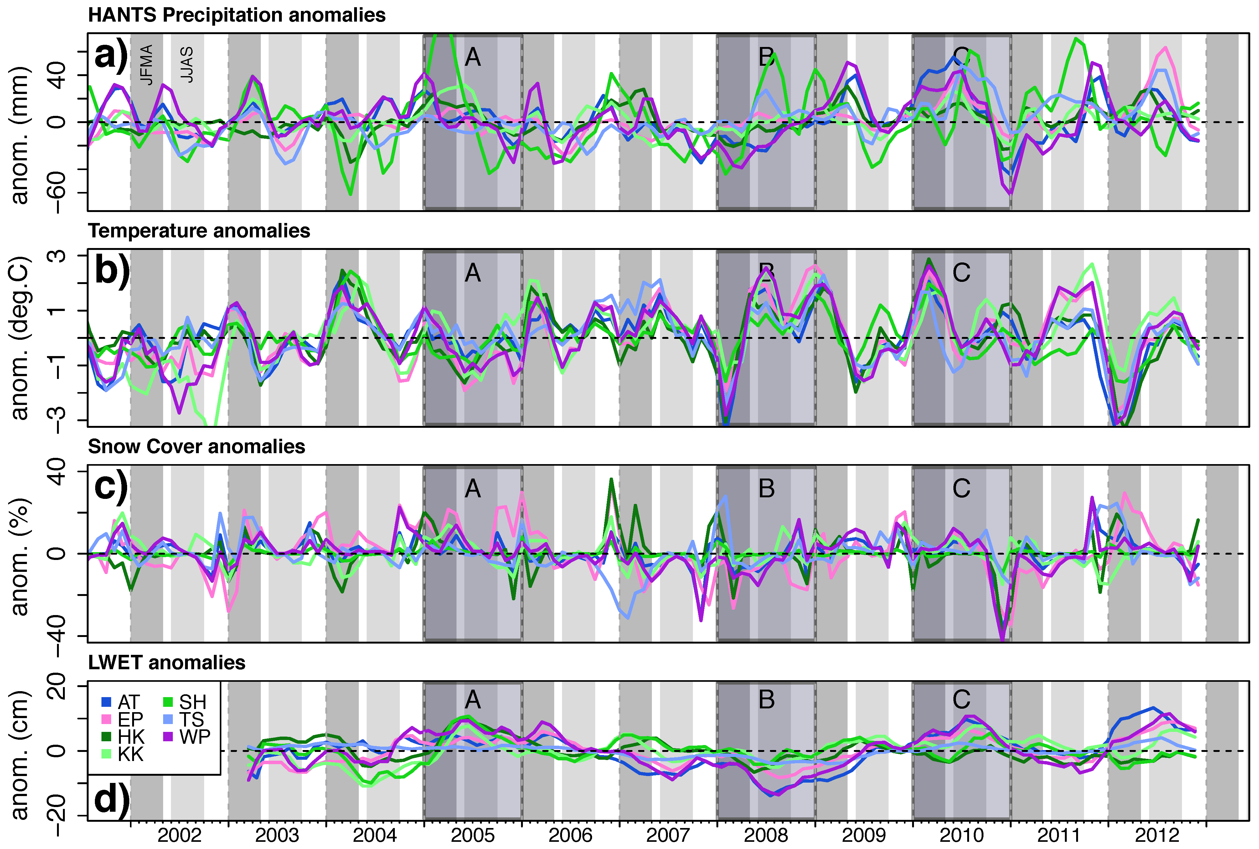
5.1. Mean Patterns and Inter-Annual Variability

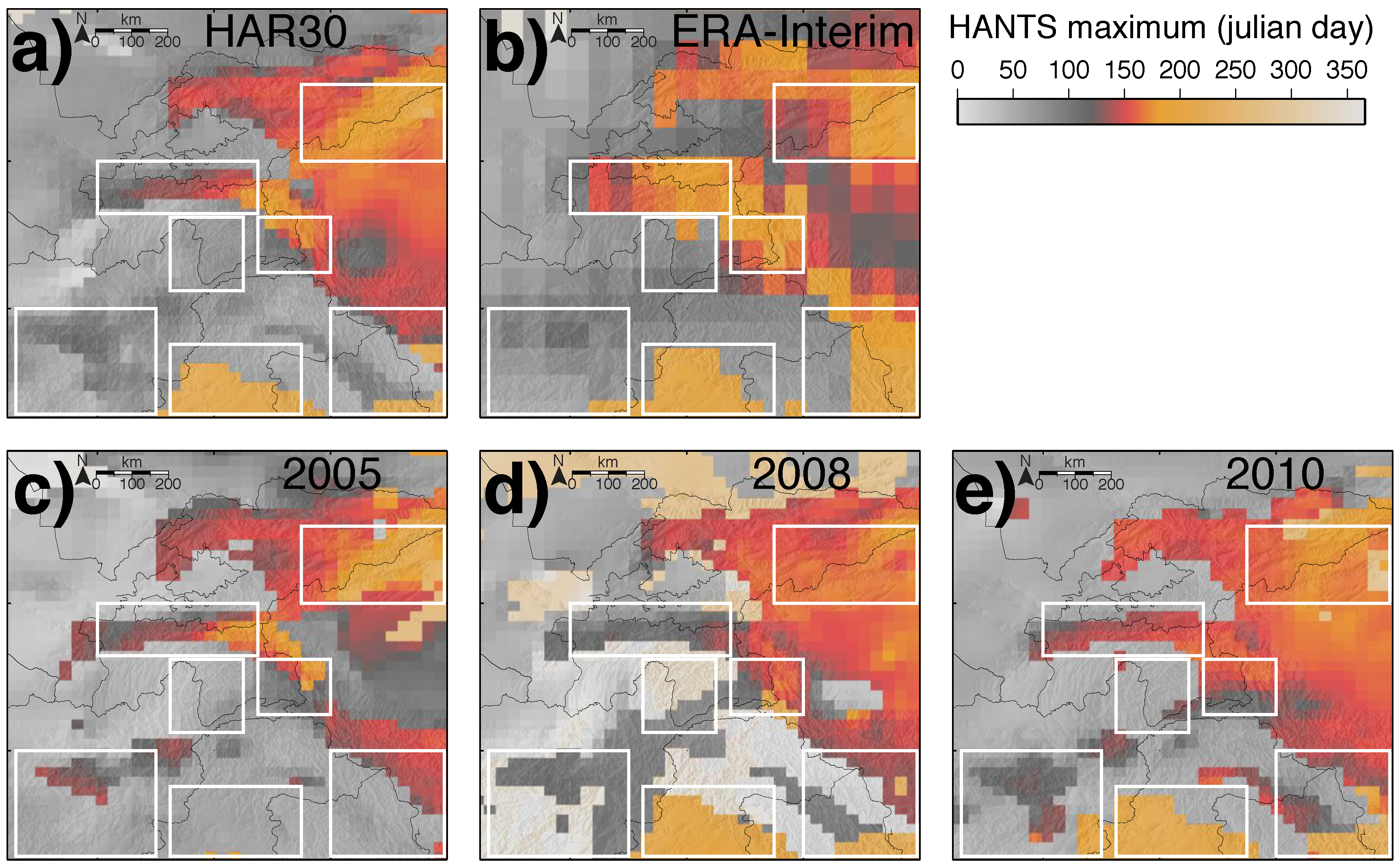

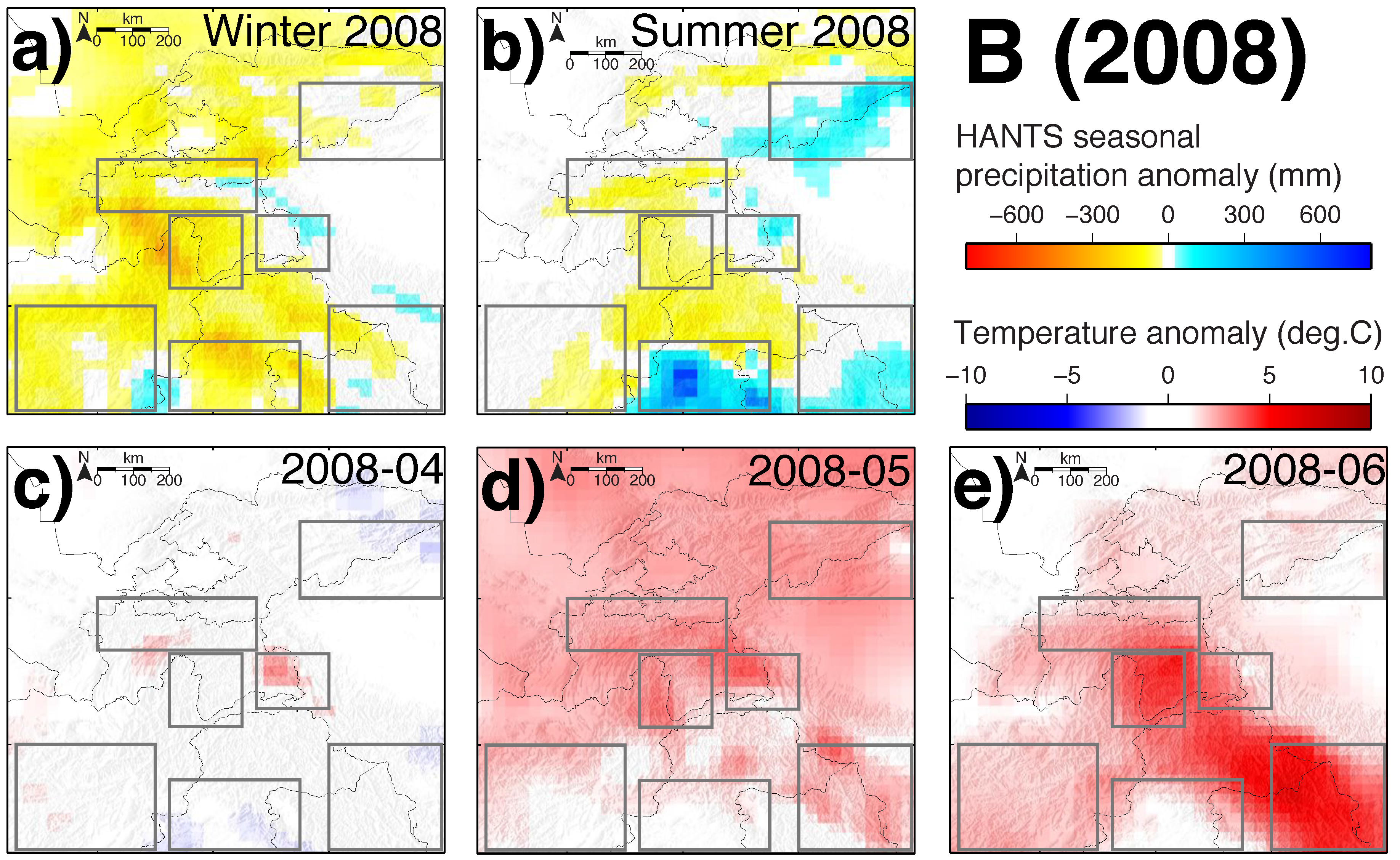
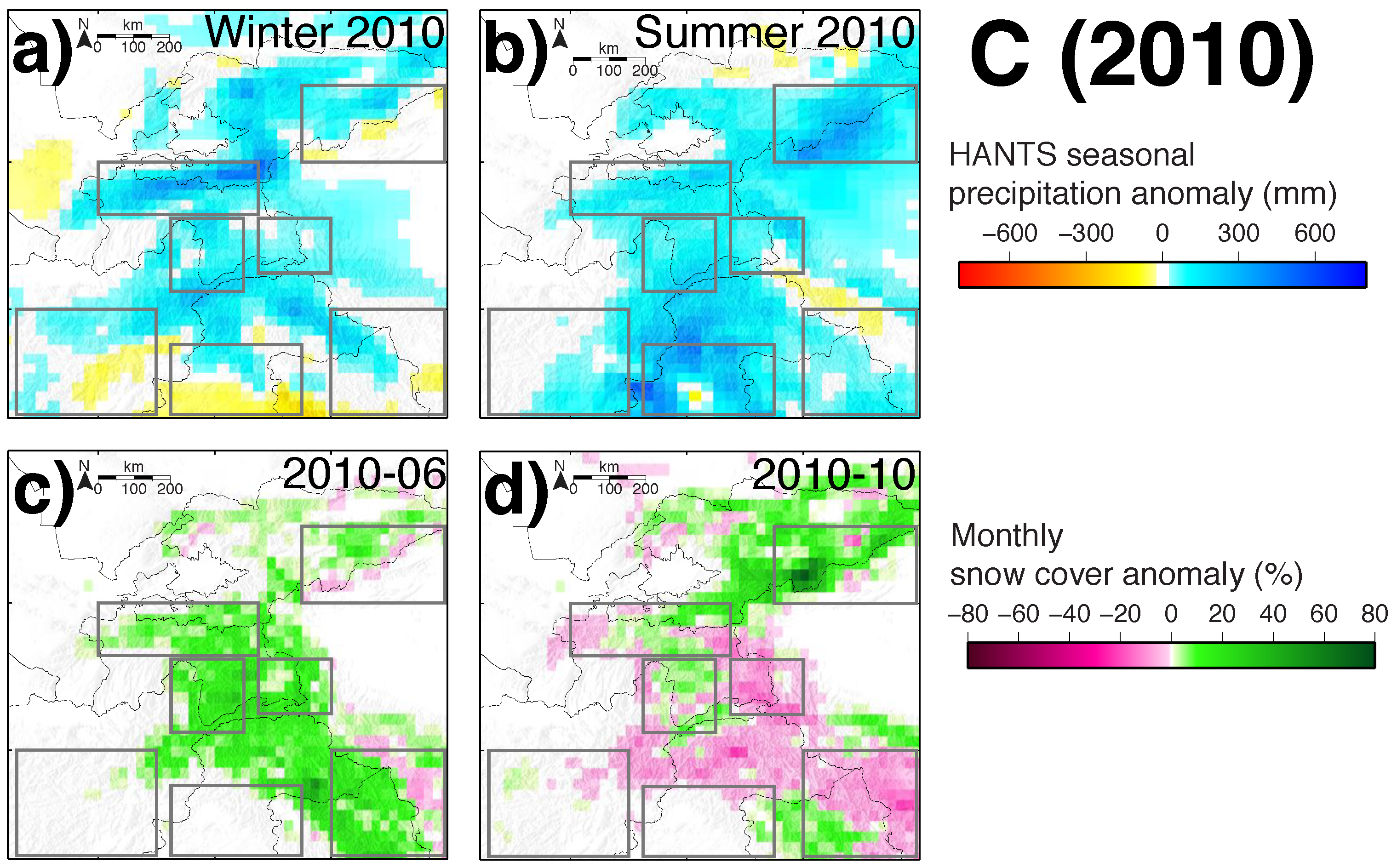
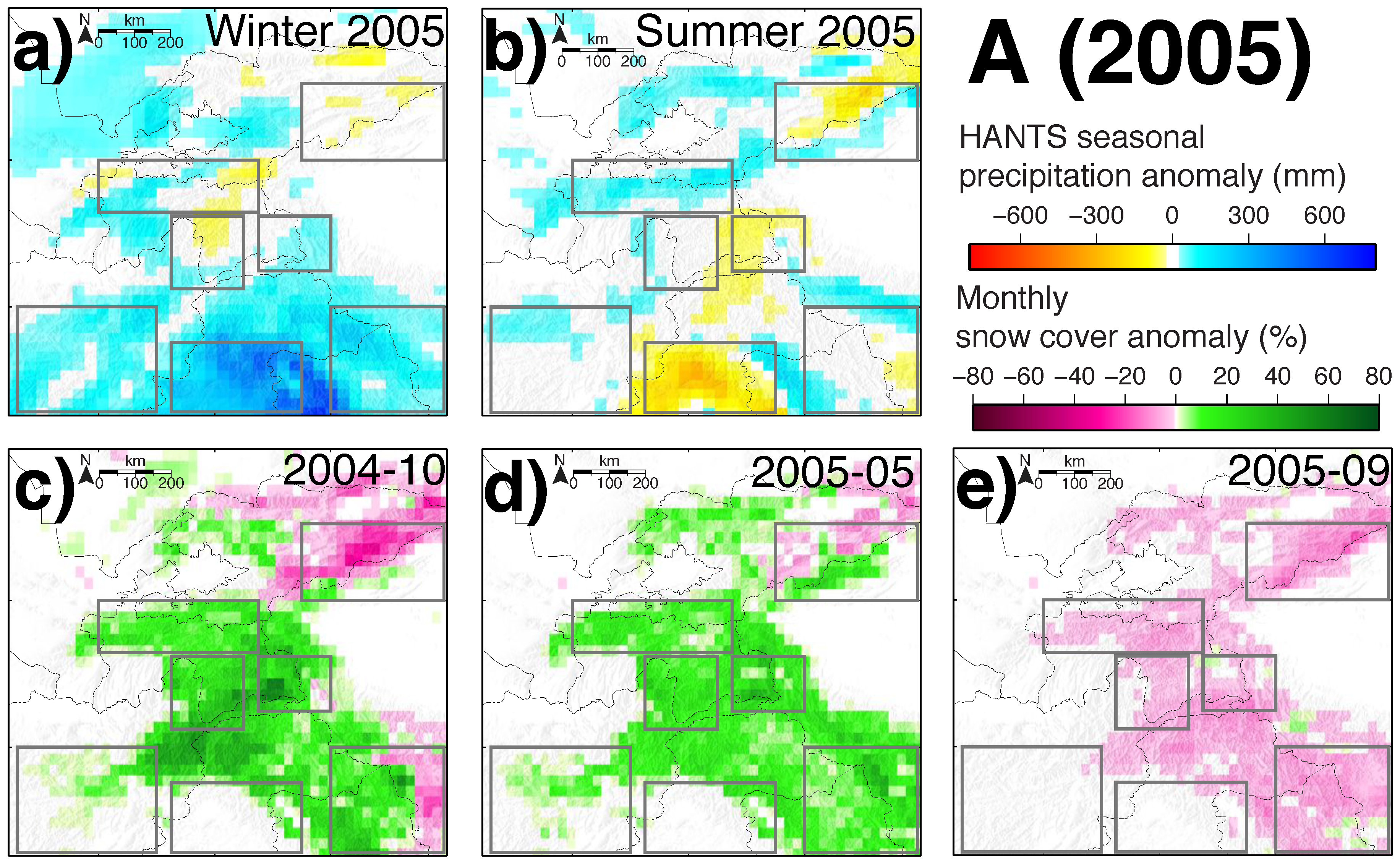
5.2. Individual Years


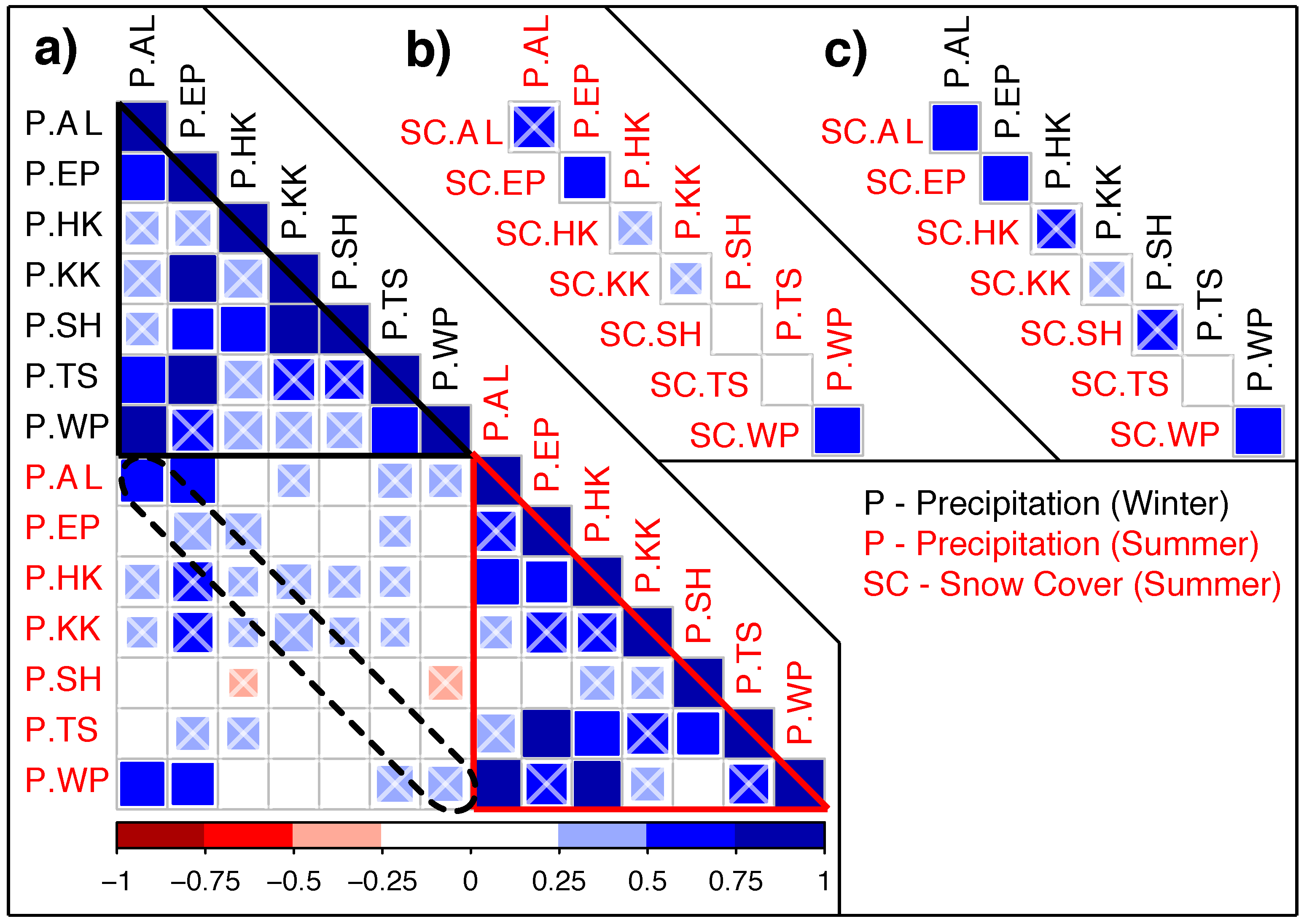
5.3. Spatial Correlation of Winter and Summer Precipitation

6. Discussion
6.1. HANTS Precipitation and Interplay of Atmospheric Circulations
6.2. Inter-Annual Weather Variability
6.3. Impacts on Glacier Evolution
6.4. Impacts on Hazards
7. Conclusions
Acknowledgments
Author Contributions
Conflicts of Interest
References
- Pohl, E.; Knoche, M.; Gloaguen, R.; Andermann, C.; Krause, P. The hydrological cycle in the high Pamir Mountains: How temperature and seasonal precipitation distribution influence stream flow in the Gunt catchment, Tajikistan. Earth Surf. Dyn. Discuss. 2014, 2, 1155–1215. [Google Scholar] [CrossRef]
- Fuchs, M.C.; Gloaguen, R.; Pohl, E. Tectonic and climatic forcing on the Panj river system during the Quaternary. Int. J. Earth Sci. 2013, 102, 1985–2003. [Google Scholar] [CrossRef] [Green Version]
- Tahir, A.A.; Chevallier, P.; Arnaud, Y.; Ahmad, B. Snow cover dynamics and hydrological regime of the Hunza River basin, Karakoram Range, Northern Pakistan. Hydrol. Earth Syst. Sci. Discuss. 2011, 8, 2821–2860. [Google Scholar] [CrossRef]
- Aizen, V.B.; Mayewski, P.A.; Aizen, E.M.; Joswiak, D.R.; Surazakov, A.B.; Kaspari, S.; Grigholm, B.; Krachler, M.; Handley, M.; Finaev, A. Stable-isotope and trace element time series from Fedchenko glacier (Pamirs) snow/firn cores. J. Glaciol. 2009, 55, 275–291. [Google Scholar] [CrossRef]
- Immerzeel, W.; Droogers, P.; de Jong, S.; Bierkens, M. Large-scale monitoring of snow cover and runoff simulation in Himalayan river basins using remote sensing. Remote Sens. Environ. 2009, 113, 40–49. [Google Scholar] [CrossRef]
- Lutz, A.F.; Immerzeel, W.W.; Shrestha, A.B.; Bierkens, M.F.P. Consistent increase in High Asia’s runoff due to increasing glacier melt and precipitation. Nat. Clim. Chang. 2014, 4, 587–592. [Google Scholar] [CrossRef]
- Hagg, W.; Braun, L.; Kuhn, M.; Nesgaard, T. Modelling of hydrological response to climate change in glacierized Central Asian catchments. J. Hydrol. 2007, 332, 40–53. [Google Scholar] [CrossRef] [Green Version]
- Sorg, A.; Bolch, T.; Stoffel, M.; Solomina, O.; Beniston, M. Climate change impacts on glaciers and runoff in Tien Shan (Central Asia). Nat. Clim. Chang. 2012, 2, 725–731. [Google Scholar] [CrossRef]
- Bookhagen, B.; Burbank, D.W. Toward a complete Himalayan hydrological budget: Spatiotemporal distribution of snowmelt and rainfall and their impact on river discharge. J. Geophys. Res. 2010, 115, 1–25. [Google Scholar] [CrossRef]
- Palazzi, E.; Hardenberg, J.V.; Provenzale, A. Precipitation in the Hindu-Kush Karakoram Himalaya: Observations and future scenarios. J. Geophys. Res.: Atmos. 2013, 118, 85–100. [Google Scholar]
- Skofronick-Jackson, G.; Weinman, J. A physical model to determine snowfall over land by microwave radiometry. IEEE Trans. Geosci. Remote Sens. 2004, 42, 1047–1058. [Google Scholar] [CrossRef]
- Prigent, C. Precipitation retrieval from space: An overview. Comptes Rendus Geosci. 2010, 342, 380–389. [Google Scholar] [CrossRef]
- Unger-Shayesteh, K.; Vorogushyn, S.; Farinotti, D.; Gafurov, A.; Duethmann, D.; Mandychev, A.; Merz, B. What do we know about past changes in the water cycle of Central Asian headwaters? A review. Glob. Planet. Chang. 2013, 110, 4–25. [Google Scholar] [CrossRef]
- Zech, R.; Abramowski, U.; Glaser, B.; Sosin, P.; Kubik, P.; Zech, W. Late Quaternary glacial and climate history of the Pamir Mountains derived from cosmogenic be exposure ages. Quat. Res. 2005, 64, 212–220. [Google Scholar] [CrossRef]
- Röhringer, I.; Zech, R.; Abramowski, U.; Sosin, P.; Aldahan, A.; Kubik, P.W.; Zöller, L.; Zech, W. The late Pleistocene glaciation in the Bogchigir Valleys (Pamir, Tajikistan) based on 10Be surface exposure dating. Quat. Res. 2012, 78, 590–597. [Google Scholar] [CrossRef]
- Seong, Y.B.; Owen, L.a.; Yi, C.; Finkel, R.C. Quaternary glaciation of Muztag Ata and Kongur Shan: Evidence for glacier response to rapid climate changes throughout the Late Glacial and Holocene in westernmost Tibet. Geol. Soc. Am. Bull. 2009, 121, 348–365. [Google Scholar] [CrossRef]
- Maussion, F.; Scherer, D.; Mölg, T.; Collier, E.; Curio, J.; Finkelnburg, R. Precipitation seasonality and variability over the Tibetan Plateau as resolved by the High Asia reanalysis. J. Clim. 2014, 27, 1910–1927. [Google Scholar] [CrossRef]
- Gardelle, J.; Berthier, E.; Arnaud, Y. Slight mass gain of Karakoram glaciers in the early Twenty-First century. Nat. Geosci. 2012, 5, 322–325. [Google Scholar] [CrossRef]
- Gardelle, J.; Berthier, E.; Arnaud, Y.; Kääb, A. Region-wide glacier mass balances over the Pamir-Karakoram-Himalaya during 1999–2011. Cryosphere 2013, 7, 1263–1286. [Google Scholar] [CrossRef] [Green Version]
- Mölg, T.; Maussion, F.; Yang, W.; Scherer, D. The footprint of Asian monsoon dynamics in the mass and energy balance of a Tibetan glacier. Cryosphere 2012, 6, 1445–1461. [Google Scholar] [CrossRef]
- de Jong, R.; de Bruin, S.; de Wit, A.; Schaepman, M.E.; Dent, D.L. Analysis of monotonic greening and browning trends from global NDVI time-series. Remote Sens. Environ. 2011, 115, 692–702. [Google Scholar] [CrossRef] [Green Version]
- Roerink, G.J.; Menenti, M.; Verhoef, W. Reconstructing cloudfree NDVI composites using Fourier analysis of time series. Int. J. Remote Sens. 2000, 21, 1911–1917. [Google Scholar] [CrossRef]
- Li, W.; Luo, C.; Wang, D.; Lei, T. Diurnal variations of precipitation over the South China Sea. Meteorol. Atmos. Phys. 2010, 109, 33–46. [Google Scholar] [CrossRef]
- Justino, F.; Setzer, A.; Bracegirdle, T.J.; Mendes, D.; Grimm, A.; Dechiche, G.; Schaefer, C.E.G.R. Harmonic analysis of climatological temperature over Antarctica: Present day and greenhouse warming perspectives. Int. J. Climatol. 2011, 31, 514–530. [Google Scholar] [CrossRef]
- Xu, Y.; Shen, Y.; Wu, Z. Spatial and temporal variations of land surface temperature over the Tibetan Plateau based on Harmonic analysis. Mount. Res. Dev. 2013, 33, 85–94. [Google Scholar] [CrossRef]
- Horn, L.H.; Bryson, R.A. Harmonic analysis of the annual March of precipitation over the United States 1. Ann. Assoc. Am. Geogr. 1960, 50, 157–171. [Google Scholar] [CrossRef]
- Kirkyla, K.I.; Hameed, S. Harmonic analysis of the seasonal cycle in precipitation over the United States: A comparison between observations and a general circulation model. J. Clim. 1989, 2, 1463–1475. [Google Scholar] [CrossRef]
- Kadioğlu, M.; Öztürk, N.; Erdun, H.; Şen, Z. On the precipitation climatology of Turkey by harmonic analysis. Int. J. Climatol. 1999, 19, 1717–1728. [Google Scholar] [CrossRef]
- Tarawneh, Q. Harmonic analysis of precipitation climatology in Saudi Arabia. Theor. Appl. Climatol. 2015. [Google Scholar] [CrossRef]
- Seiler, R. Analyse linearer Trends in der Phänologie multimodaler Vegetation, Auswertung von NDVI Zeitreihen für das Niger Binnendelta (Rep. Mali / Westafrika) (in German). In Proceedings of the 32nd Scientific–Technical Annual Meeting of the DGPF (Deutsche Gesellschaft für Photogrammetrie, Fernerkundung und Geoinformation e.V.), Potsdam, Germany, 14–17 March 2012; Volume 21, pp. 65–74.
- Seiler, R.; Gloaguen, R. (Non-)linear phenological trends in an ecosystem with multiple growing seasons derived from AVHRR-NDVI time series. In Proceedings of the 2012 IEEE International Geoscience and Remote Sensing Symposium (IGARSS), Munich, Germany, 22–27 July 2012; pp. 6789–6792.
- Yao, T.; Thompson, L.; Yang, W.; Yu, W.; Gao, Y.; Guo, X.; Yang, X.; Duan, K.; Zhao, H.; Xu, B.; et al. Different glacier status with atmospheric circulations in Tibetan Plateau and surroundings. Nat. Clim. Chang. 2012, 2, 663–667. [Google Scholar] [CrossRef]
- Fuchs, M.C.; Gloaguen, R.; Krbetschek, M.; Szulc, A. Rates of river incision across the main tectonic units of the Pamir identified using optically stimulated luminescence dating of fluvial terraces. Geomorphology 2014, 216, 79–92. [Google Scholar] [CrossRef] [Green Version]
- Huffman, G.J. Estimates of Root-Mean-Square Random Error for finite samples of estimated precipitation. J. Appl. Meteorol. 1997, 36, 1191–1201. [Google Scholar] [CrossRef]
- Huffman, G.J.; Adler, R.F.; Arkin, P.; Chang, A.; Ferraro, R.; Gruber, A.; Janowiak, J.; McNab, A.; Rudolf, B.; Schneider, U. The Global Precipitation Climatology Project (GPCP) combined precipitation dataset. Bull. Am. Meteorol. Soc. 1997, 78, 5–20. [Google Scholar] [CrossRef]
- Huffman, G.J.; Adler, R.F.; Bolvin, D.T.; Gu, G.; Nelkin, E.J.; Bowman, K.P.; Hong, Y.; Stocker, E.F.; Wolff, D.B. The TRMM Multisatellite Precipitation Analysis (TMPA): Quasi-global, multiyear, combined-sensor precipitation estimates at fine scales. J. Hydrometeorol. 2007, 8, 38. [Google Scholar] [CrossRef]
- Yin, Z.Y. Using a geographic information system to improve Special Sensor Microwave Imager precipitation estimates over the Tibetan Plateau. J. Geophys. Res. 2004, 109, D03110. [Google Scholar] [CrossRef]
- Kamal-Heikman, S.; Derry, L.A.; Stedinger, J.R.; Duncan, C.C. A simple predictive tool for lower Brahmaputra River Basin monsoon flooding. Earth Interact. 2007, 11, 1–11. [Google Scholar] [CrossRef]
- Prigent, C. Precipitation retrieval from space: An overview. Comptes Rendus Geosci. 2010, 342, 380–389. [Google Scholar] [CrossRef]
- Dee, D.P.; Uppala, S.M.; Simmons, A.J.; Berrisford, P.; Poli, P.; Kobayashi, S.; Andrae, U.; Balmaseda, M.A.; Balsamo, G.; Bauer, P.; et al. The ERA-Interim reanalysis: Configuration and performance of the data assimilation system. Q. J. R. Meteorol. Soc. 2011, 137, 553–597. [Google Scholar] [CrossRef]
- National Centers for Environmental Prediction–NOAA, U.S. Department of Commerce, National Weather Service (NWS). NCEP FNL Operational Model Global Tropospheric Analyses, Continuing from July 1999. Available online: http://rda.ucar.edu/datasets/ds083.2/#access (accessed on 10 July 2015).
- Skamarock, W.C.; Klemp, J.B. A time-split nonhydrostatic atmospheric model for weather research and forecasting applications. J. Comput. Phys. 2008, 227, 3465–3485. [Google Scholar] [CrossRef]
- Hall, D.K.; Salomonson, V.V.; Riggs, G.A. MODIS/Terra Snow Cover Monthly L3 Global 0.05Deg CMG, Version 5. [MOD10CM]; National Snow and Ice Data Center: Boulder, CO, USA, 2006. [Google Scholar]
- Dietz, A.; Conrad, C.; Kuenzer, C.; Gesell, G.; Dech, S. Identifying changing snow cover characteristics in Central Asia between 1986 and 2014 from remote sensing data. Remote Sens. 2014, 6, 12752–12775. [Google Scholar] [CrossRef]
- Hall, D.K.; Salomonson, V.V.; Riggs, G.A. MODIS/Terra Snow Cover Daily L3 Global 0.05deg CMG V005. [MOD10C1]; National Snow and Ice Data Center: Boulder, CO, USA, 2006. [Google Scholar]
- Landerer, F.W.; Swenson, S.C. Accuracy of scaled GRACE terrestrial water storage estimates. Water Resour. Res. 2012, 48, W04531. [Google Scholar] [CrossRef]
- Swenson, S.; Wahr, J. Post-processing removal of correlated errors in GRACE data. Geophys. Res. Lett. 2006, 33, L08402. [Google Scholar] [CrossRef]
- Dahle, C.; Flechtner, F.; Gruber, C.; König, D.; König, R.; Michalak, G.; Neumayer, K.H. GFZ GRACE Level-2 Processing Standards Document for Level-2 Product Release 0005: Revised Edition; Technical Report; Deutsches GeoForschungsZentrum GFZ: Potsdam, Germany, 2013. [Google Scholar]
- Lettenmaier, D.P.; Famiglietti, J.S. Hydrology: Water from on high. Nature 2006, 444, 562–563. [Google Scholar] [CrossRef] [PubMed]
- Syed, T.H.; Famiglietti, J.S.; Rodell, M.; Chen, J.; Wilson, C.R. Analysis of terrestrial water storage changes from GRACE and GLDAS. Water Resour. Res. 2008. [Google Scholar] [CrossRef]
- Ramillien, G.; Famiglietti, J.S.; Wahr, J. Detection of continental hydrology and glaciology signals from GRACE: A review. Surv. Geophys. 2008, 29, 361–374. [Google Scholar] [CrossRef]
- Jacob, T.; Wahr, J.; Pfeffer, W.T.; Swenson, S. Recent contributions of glaciers and ice caps to sea level rise. Nature 2012, 482, 514–8. [Google Scholar] [CrossRef] [PubMed]
- Guha-Sapir, D.; Below, R.; Hoyois, P. EM-DAT: International Disaster Database; Technical Report; Université Catholique de Louvain: Brussels, Belgium, 2014. [Google Scholar]
- Beekma, J.; Fiddes, J. Floods and droughts : The Afghan water paradox. In Afghanistan Human Development Report 2011; Kabul University (UNDP-Afghanistan): Kabul, Afghanistan, 2011; pp. 1–30. [Google Scholar]
- Mahmood, A.; Faisal, N.; Jameel, A. Special Report on Pakistan’s Monsoon 2011 Rainfall; Technical Report January; Pakistan Meteorological Department: Karachi, Pakistan, 2012. [Google Scholar]
- Houze, R.A.; Rasmussen, K.L.; Medina, S.; Brodzik, S.R.; Romatschke, U. Anomalous atmospheric events leading to the summer 2010 floods in Pakistan. Bull. Am. Meteorol. Soc. 2011, 92, 291–298. [Google Scholar] [CrossRef]
- Kapnick, S.B.; Delworth, T.L.; Ashfaq, M.; Malyshev, S.; Milly, P.C.D. Snowfall less sensitive to warming in Karakoram than in Himalayas due to a unique seasonal cycle. Nat. Geosci. 2014, 7, 834–840. [Google Scholar] [CrossRef]
- Immerzeel, W.W.; van Beek, L.P.H.; Bierkens, M.F.P. Climate change will affect the Asian water towers. Science 2010, 328, 1382–1385. [Google Scholar] [CrossRef] [PubMed]
- Harr, R.D. Some characteristics and consequences of snowmelt during rainfall in western Oregon. J. Hydrol. 1981, 53, 277–304. [Google Scholar] [CrossRef]
- World Health Organization. Pakistan Floods Situation Report#F-1-2008 (Aug 3–5, 2008); Technical Report; World Health Organization–Country Office, National Institute of Health: Islamabad, Pakistan, 2008. [Google Scholar]
- Fujita, K.; Ageta, Y. Effect of summer accumulation on glacier mass balance on the Tibetan Plateau revealed by mass-balance model. J. Glaciol. 2000, 46, 244–252. [Google Scholar] [CrossRef]
- Liu, X.; Herzschuh, U.; Wang, Y.; Kuhn, G.; Yu, Z. Glacier fluctuations of Muztagh Ata and temperature changes during the late Holocene in westernmost Tibetan Plateau, based on glaciolacustrine sediment records. Geophys. Res. Lett. 2014, 41, 6265–6273. [Google Scholar] [CrossRef]
- Khromova, T.; Osipova, G.; Tsvetkov, D.; Dyurgerov, M.; Barry, R. Changes in glacier extent in the eastern Pamir, Central Asia, determined from historical data and ASTER imagery. Remote Sens. Environ. 2006, 102, 24–32. [Google Scholar] [CrossRef]
- Gruber, F.E.; Mergili, M. Regional-scale analysis of high-mountain multi-hazard and risk indicators in the Pamir (Tajikistan) with GRASS GIS. Nat. Hazards Earth Syst. Sci. 2013, 13, 2779–2796. [Google Scholar] [CrossRef]
- Hou, A.Y.; Kakar, R.K.; Neeck, S.; Azarbarzin, A.A.; Kummerow, C.D.; Kojima, M.; Oki, R.; Nakamura, K.; Iguchi, T. The Global Precipitation Measurement Mission. Bull. Am. Meteorol. Soc. 2014, 95, 701–722. [Google Scholar] [CrossRef]
- R Core Team. R: A Language and Environment for Statistical Computing; R Foundation for Statistical Computing: Vienna, Austria, 2014. [Google Scholar]
- Hijmans, R.J. raster: Geographic Data Analysis and Modeling, 2015; R Package Version 2.4-15. Available online: http://CRAN.R-project.org/package=raster (accessed on 29 July 2015).
- Bivand, R.; Keitt, T.; Rowlingson, B. rgdal: Bindings for the Geospatial Data Abstraction Library, 2015; R Package Version 1.0-4. Available online: http://CRAN.R-project.org/package=rgdal (accessed on 29 July 2015).
© 2015 by the authors; licensee MDPI, Basel, Switzerland. This article is an open access article distributed under the terms and conditions of the Creative Commons Attribution license (http://creativecommons.org/licenses/by/4.0/).
Share and Cite
Pohl, E.; Gloaguen, R.; Seiler, R. Remote Sensing-Based Assessment of the Variability of Winter and Summer Precipitation in the Pamirs and Their Effects on Hydrology and Hazards Using Harmonic Time Series Analysis. Remote Sens. 2015, 7, 9727-9752. https://doi.org/10.3390/rs70809727
Pohl E, Gloaguen R, Seiler R. Remote Sensing-Based Assessment of the Variability of Winter and Summer Precipitation in the Pamirs and Their Effects on Hydrology and Hazards Using Harmonic Time Series Analysis. Remote Sensing. 2015; 7(8):9727-9752. https://doi.org/10.3390/rs70809727
Chicago/Turabian StylePohl, Eric, Richard Gloaguen, and Ralf Seiler. 2015. "Remote Sensing-Based Assessment of the Variability of Winter and Summer Precipitation in the Pamirs and Their Effects on Hydrology and Hazards Using Harmonic Time Series Analysis" Remote Sensing 7, no. 8: 9727-9752. https://doi.org/10.3390/rs70809727