Article

Identification of Forested Landslides Using LiDar Data, Object-based Image Analysis, and Machine Learning Algorithms

1
Faculty of Information Engineering, China University of Geosciences, Wuhan 430074, China
2
Faculty of Computer Science and Hubei Key Laboratory of Intelligent Geo-Information Processing, China University of Geosciences, Wuhan 430074, China
3
Faculty of Geo-Information Science and Earth Observation (ITC), University of Twente, 7500 Enschede, The Netherlands
4
Institute for Remote Sensing Method, China Aero Geophysical Survey and Remote Sensing Center for Land and Resources, Beijing 100083, China
*
Author to whom correspondence should be addressed.
Remote Sens. 2015, 7(8), 9705-9726; https://doi.org/10.3390/rs70809705
Submission received: 25 April 2015 / Revised: 13 July 2015 / Accepted: 20 July 2015 / Published: 30 July 2015

Abstract

:
For identification of forested landslides, most studies focus on knowledge-based and pixel-based analysis (PBA) of LiDar data, while few studies have examined (semi-) automated methods and object-based image analysis (OBIA). Moreover, most of them are focused on soil-covered areas with gentle hillslopes. In bedrock-covered mountains with steep and rugged terrain, it is so difficult to identify landslides that there is currently no research on whether combining semi-automated methods and OBIA with only LiDar derivatives could be more effective. In this study, a semi-automatic object-based landslide identification approach was developed and implemented in a forested area, the Three Gorges of China. Comparisons of OBIA and PBA, two different machine learning algorithms and their respective sensitivity to feature selection (FS), were first investigated. Based on the classification result, the landslide inventory was finally obtained according to (1) inclusion of holes encircled by the landslide body; (2) removal of isolated segments, and (3) delineation of closed envelope curves for landslide objects by manual digitizing operation. The proposed method achieved the following: (1) the filter features of surface roughness were first applied for calculating object features, and proved useful; (2) FS improved classification accuracy and reduced features; (3) the random forest algorithm achieved higher accuracy and was less sensitive to FS than a support vector machine; (4) compared to PBA, OBIA was more sensitive to FS, remarkably reduced computing time, and depicted more contiguous terrain segments; (5) based on the classification result with an overall accuracy of 89.11% ± 0.03%, the obtained inventory map was consistent with the referenced landslide inventory map, with a position mismatch value of 9%. The outlined approach would be helpful for forested landslide identification in steep and rugged terrain.

Graphical Abstract

1. Introduction

The Yangtze Three Gorges area of China has more than 2500 unstable slope localities, and often suffers from landslide events [1,2,3]. The construction of the Three Gorges dam has increased the probability of geological disasters [2,4] that pose a serious threat to people’s lives and property around the Three Gorges Reservoir. Preparation of landslide inventories is absolutely necessary to help quantify landslide hazard and to assess risk [2,5,6,7,8,9,10,11]. The Three Gorges area is characterized by steep and rugged terrain with heavy vegetation cover, often obscuring or subduing morphologic features indicative of landslides [12,13]. The landscape makes it particularly challenging to identify landslides using optical and aerial photographs, synthetic aperture radar (SAR) images, high spatial resolution multispectral images, moderate resolution digital terrain models (DTMs), and very high resolution (VHR) satellite images [6,14,15,16,17,18,19,20,21,22,23,24,25,26,27,28,29,30].
Light detection and ranging (LiDar) technology can obtain high resolution topographic data and penetrate vegetation, measuring features subdued by the rugged and forested terrain [11]. LiDar has proven to be a powerful and promising tool to detect landslides and map features under dense vegetation in many studies [31,32,33,34,35,36,37,38,39,40]. A range of LiDar derivatives, including DTMs, shaded relief, slope, aspect, and surface roughness, have been widely used for qualitative visual interpretation and quantitative statistical analysis of landslides [12,32,41,42,43,44,45,46,47].
Pixel-based and object-based methods are the two general image analysis approaches for terrain evaluation. With increasing availability and wide utilization of sub-meter imagery, object-based image analysis (OBIA) has become the most basic means to process VHR imagery [48]. Unlike pixel-based analysis (PBA), OBIA can be applied at different scales. Depending on the selected application, the underlying input imagery, and the environment under analysis, objects of different sizes that depict different land surface features can be produced. OBIA can derive additional geometry and contextual semantic features that are potentially useful for classification studies [49]. Optical images evaluated with OBIA have been increasingly used for landslide inventory mapping, effectively detecting unvegetated landslides [9,22,28,50,51,52]. Furthermore, Stumpf and Kerle [28] have successfully combined VHR remote sensing imagery, OBIA, a feature selection method, and a random forest (RF) algorithm for unvegetated landslide mapping. OBIA using LiDar data has also become a useful alternative in heavily forested areas because of the difficulty of using optical image-based analysis in rugged and vegetated terrain.
Until now, landslide investigations using LiDar derivatives have primarily focused on knowledge-based and pixel analysis methods [39,42]. However, the use of OBIA for topographic data has received growing attention because of increasing availability of high-resolution DTM data. Martha et al. [22,51] used optical images for segmentation and auxiliary elevation data for OBIA-based landslide detection. Anders et al. [53] used LiDar DTM-derived features for OBIA-based geomorphological change detection. Eisank et al. [54] used DTM data for OBIA-based drumlin delineation. Only Van den Eeckhaut et al. [39] have used the support vector machine (SVM) algorithm and LiDar derivatives alone for object-based mapping of landslides in forested terrain, and only on soil-covered areas with gentle hillslopes. In a word, this study was mainly inspired by Stumpf and Kerle [28] and Van den Eeckhaut et al. [39]. For bedrock-covered mountains with steep and rugged terrain, it is more difficult to identify landslides because: (1) the main scarp is either indistinct or difficult to distinguish from surrounding objects; (2) landslide-affected areas have similar surface roughness to the surrounding non-landslide areas because of bedrock outcrop; and (3) anthropogenic disturbances alter and weaken the landslide signatures. It has not been examined whether combining semi-automated methods and OBIA with only LiDar derivatives could be effective. Moreover, comparisons of PBA and OBIA, machine learning algorithms (MLAs), and their sensitivity to the feature selection method for landslide recognition in rugged forested terrain have not been investigated.
In this study, a semi-automatic landslide identification procedure, which combines LiDar data, OBIA, a feature selection method, and two MLAs (RF and SVM), was developed and implemented in a forested area with steep and rugged terrain, the Three Gorges area of China. First, the following pixel features were generated; (1) topographic features: DTM, slope, aspect, and surface roughness; (2) texture features: DTM, slope, aspect, and surface roughness textures based on four texture directions and aspect direction; (3) filter features: the moving average and standard deviation (stdev) filter features of DTM, slope, aspect, and surface roughness. LiDar DTM data were then used alone for image segmentation, and all the above LiDar derivative maps were applied to calculate the object features. A wrapper feature selection method based on RF was applied to assess and select the features, resulting in an optimal object features subset. The classification accuracies of all features-based and the features subset-based models using RF and SVM algorithms were calculated. Also, comparisons between OBIA and the previous PBA [42], and the sensitivity of these two methods and the MLAs to the feature selection method were investigated. Van den Eeckhaut et al. [39] proposed a multi-stage procedure to identify landslides: (1) extraction of main scarps and landslide-affected areas using SVM, (2) artificial drawing of landslide flanks, (3) linking of landslide parts in to one landslide, and (4) cleaning of protrusions and isolated segments. This study referred to some ideas of this procedure and developed a simple approach. Based on the classification result, the landslide inventory map was finally obtained by the following steps: (1) inclusion of holes encircled by the spatially connective terrain segments that are classified as landslide objects; (2) removal of isolated and small segments that are located away from rivers and landslide bodies; and (3) delineation of closed envelope curves for landslide objects by manual digitizing operation.

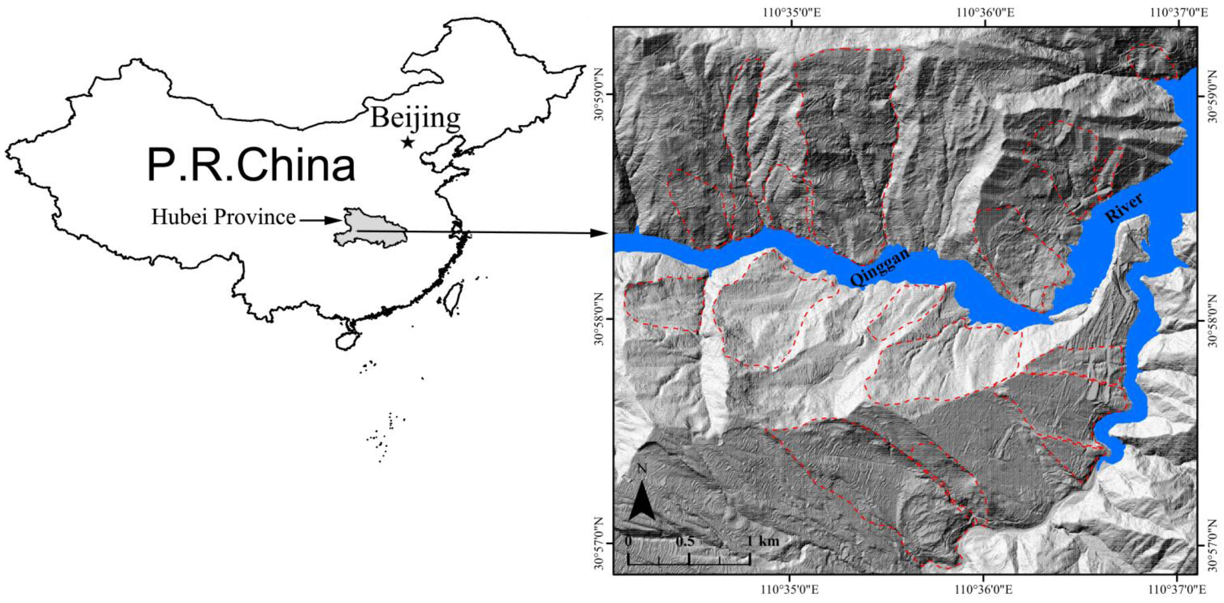
2. Study Area and Data Sources

The study covered a 21.6 km2 landslide-prone area around the town of Shazhenxi in Zigui County, and a section of the Qinggan River, which is a major branch of the Yangtze River (Figure 1). Landslides greatly affect the study area, and the referenced landslide inventory map resulted from collected landslide inventory data, extensive fieldwork, and visual interpretation of aerial images [55] and LiDar-derived topographic data [42].
The area is characterized by dense vegetation cover, steep adjoining mountains, and rugged topography at elevations of 120–851 m (derived from LiDar DTM) with bedrock outcrops such as Triassic detrital rocks (Shazhenxi Group) and Jurassic silt, lutite, pelitic siltstone, and sandstone (Niejiashan Group) [42]. Located in the subtropical and monsoonal climate zone, the weather here is mild and moist with an annual average temperature of 17–19 °C. The annual average rainfall is about 1000 mm, with concentrated and continuous rainstorms in the rainy season.
The source data for the study were 3 m resolution LiDar coverage, acquired from April to June 2009 by a Leica ALS50-II airborne laser radar system. The data encompassed the region between 110°34′4.61″E–110°37′0.17″E and 30°56′52.44″N–30°59′18.04″N (WGS_1984). The LiDar data were very reliable and fully met the requirements of this research; the data had a root mean square error of 0.20 m, and were obtained using 23 ground-truthing locations and an average laser spot density of 3.15 pts/m2 [55].
Figure 1. Shaded relief image and location of study area. Red dotted lines represent landslide boundaries. Blue area represents the Qinggan River (Revised from [42]).
Remotesensing 07 09705 g001

3. Methods

The landslide inventory map of the study area was completed using the collected landslide inventory data, extensive fieldwork, and visual interpretation of aerial images and LiDar-derived topographic data. A series of pixel features, primarily pixel-based landslide influential factors [56], were calculated from LiDar-derived DTM data. Image objects were structured from DTM images using multiresolution segmentation (MRS), and object features were extracted. The objects were then labeled as landslide (OLS) and non-landslide objects (ONLS) [28]. Objects that contained more than 50% landslide pixels were classified as OLS, and others as ONLS [28]. A wrapper feature selection method based on the RF algorithm, which utilizes the classifier as a black box to score the subsets of features based on their predictive power [57], was chosen and applied in order to reduce the dataset size. RF and SVM models were then applied to classify landslide and non-landslide objects, and the classification accuracies were assessed. Based on the classification result, the landslide inventory was finally obtained according to the following: (1) inclusion of holes surrounded by the landslide body, (2) removal of isolated and small segments that are located away from rivers and landslide bodies, and (3) delineation of closed envelope curves for OLS by manual digitizing operation. The flowchart for this process is presented in Figure 2.
Figure 2. Flowchart of the method used in this research.
Remotesensing 07 09705 g002

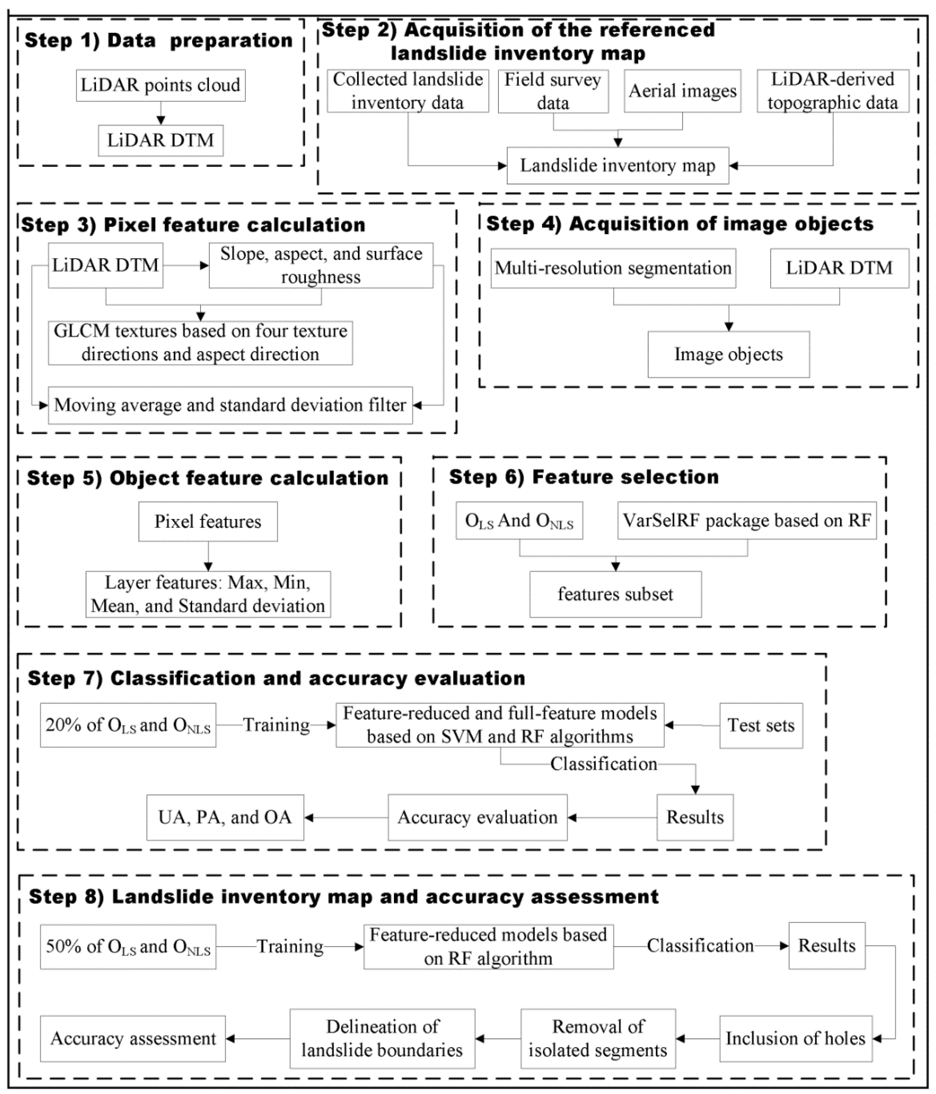
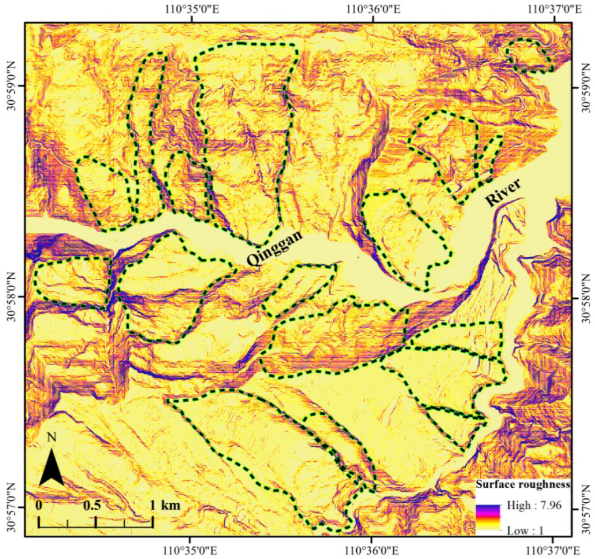
3.1. Pixel Feature Calculation

According to Chen et al. [42],the following sets of pixel features were proposed (Table 1): (1) LiDar-derived topographic features: DTM, slope, aspect, and surface roughness; (2) texture features based on the gray level co-occurrence matrix (GLCM): the mean textures of the topographic features based on four texture directions, and individual textures based on the aspect direction, mainly containing five textures—contrast, correlation, angular second moment, entropy, and homogeneity; (3) the moving average and stdev filter of the above topographic features: in the moving average and stdev filters, the value of the central pixel is replaced by the mean and stdev values, respectively, of all the pixels for a 3 × 3 pixel kernel size. The texture and filter features of surface roughness were newly added. Surface roughness (Figure 3) was calculated as the reciprocal of the cosine of the slope angle [58]. The surface roughness values at the edges of landslide-affected surfaces exhibited some changes. Landslide-affected areas had lower surface roughness compared to some non-landslide areas because of bedrock outcrop, resulting in more difficult landslide identification. A total of 52 pixel features were calculated using ArcGIS 9.3 and Matlab R2009a. Van den Eeckhaut et al. [39] used many LiDar derivatives for object feature calculation and classification, such as slope gradient, plan curvature, roughness, openness, and sky-view factor. However, to make a comparison of OBIA and the previous PBA [42], this study just focused on some basic and important LiDar derivatives, and their texture and filter features.
Figure 3. Surface roughness image and landslide locations. Black dots with green boundaries represent the landslide boundaries.
Remotesensing 07 09705 g003
Table 1. List of pixel features for object features calculation.
Pixel Feature TypeDescriptionNo.
topographic featuresDTM, slope, aspect, and surface roughness4
texture featuresThe contrast, correlation, angular second moment, entropy, and homogeneity texture of the topographic features based on four texture directions and aspect direction40
filter featuresThe moving average and standard deviation (stdev) filter of DTM, slope, aspect, and surface roughness8

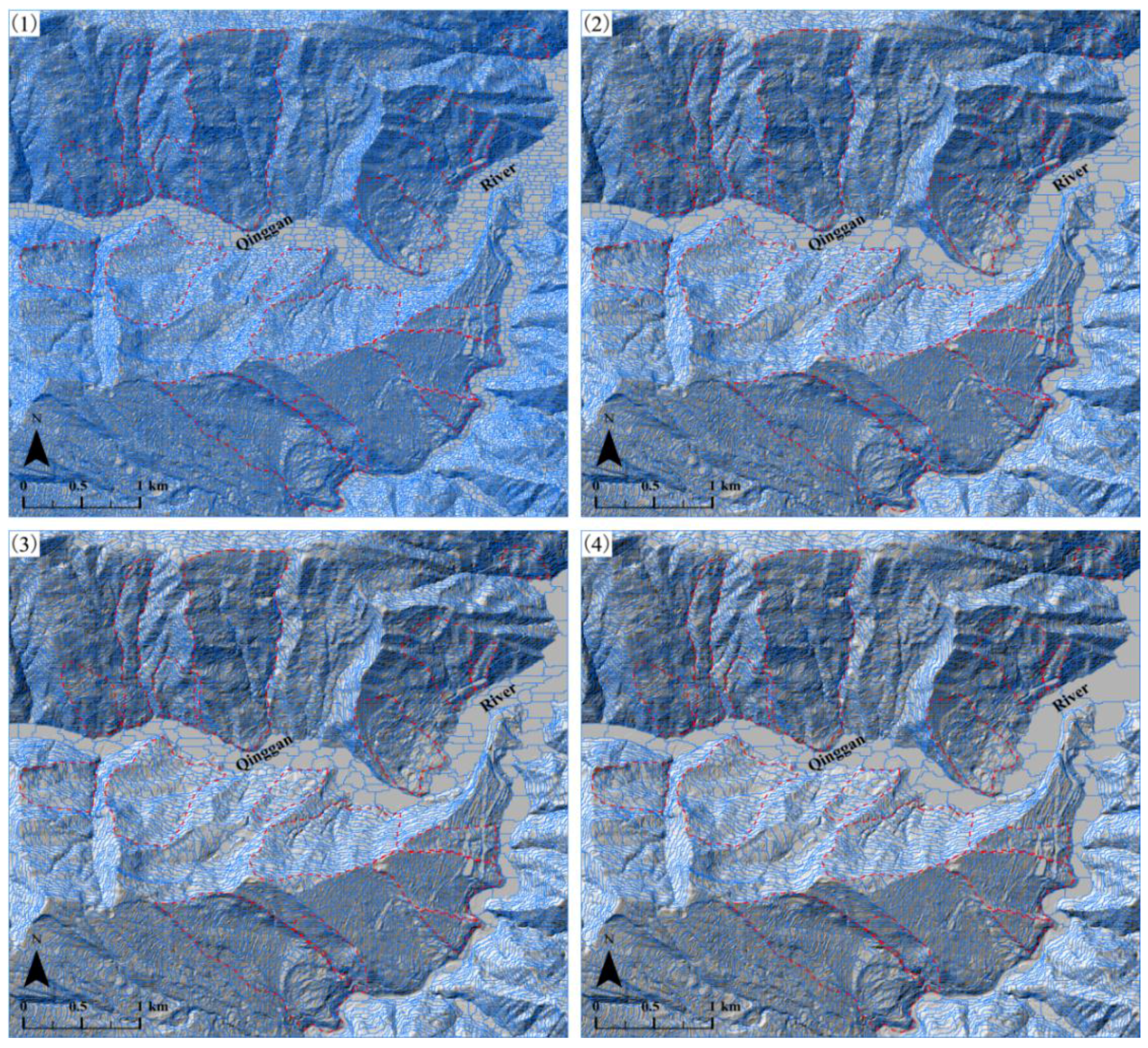
3.2. Image Segmentation

Image segmentation is the first step and a necessary prerequisite for OBIA because it determines the size and shape of image objects [49]. The selection of appropriate image segmentation parameters ultimately depends on the selected application, the underlying input imagery, and the environment under analysis [48,59,60].
There are many segmentation procedures, but MRS [61] is used by most landslide studies, and is probably the most popular and important segmentation algorithm [39,62]. MRS is a region-growing image segmentation algorithm that merges individual pixels with their most similar neighbors, until the threshold of the within-object heterogeneity is reached [63].
MRS mainly relies on three user-defined parameters: shape–color, compactness–smoothness, and scale [49]. In this study, the paired values of shape/color and compactness/smoothness represent weightings between shape and topographic information, and compactness and smoothness of the object borders. Generally, color information has higher weight; compactness and smoothness are weighted equally. The scale parameter (SP) is a key control factor for the segmentation and classification of Earth observation (EO) imagery because it controls the internal heterogeneity of image objects. Consequently, SP controls the average size of the objects, directly affecting classification accuracy [60,61,63,64,65,66]. The selection of the SP value is critical [62,67] and has become a research focus in OBIA [48]. Although some quantitative and automated approaches have been developed [51,62,68,69,70,71,72], they have not been integrated within mainstream software for OBIA [73], and SP selection is often based on an iterative trial-and-error optimization method in which the segmentation quality is visually assessed [60,74,75,76,77,78,79].
The first step of image segmentation is to select the input layers and specify their weights. In this study, an MRS algorithm was run using eCognition Developer 8 [80]. The input layers for segmentation were extremely vital because they determine the quality of the segmentation results. Other relevant OBIA researchers have successfully used VHR remote sensing imagery for unvegetated landslide mapping [28] and LiDar derivatives such as slope, roughness, and openness for forested landslide identification on soil-covered areas with gentle hillslopes [39]. However, in bedrock-covered mountains with steep and rugged terrain, the differences of topographic variables between landslide and non-landslide areas are weakened: (1) the main scarp is either indistinct or difficult to distinguish from surrounding objects; (2) landslide-affected areas have similar surface roughness to the surrounding non-landslide areas because of bedrock outcrop; and (3) anthropogenic disturbances alter and weaken the landslide signatures. Therefore, topographic variables such as slope, roughness, and so on would not be effective. Moreover, considering that the selection of input layers was often based on experience or a trial-and-error approach, which may effectively prevent the transferability of the approach developed in this study, the DTM image was first selected and investigated as the single input layer. The weights of shape/color and compactness/smoothness were first determined based on experience and a trial-and-error process by using a fixed SP. The weights of compactness and smoothness were both fixed as 0.5. Additionally, the weights of shape were selected from 0.1 to 0.4 with a step of 0.1, namely 0.9 to 0.6 for color. It was found that the weights of 0.1/0.9 for shape/color were more suitable. Stumpf and Kerle [28] used 15 different scale parameters for MRS, which may be adaptable to the scales of the objects of interest in that study, and evaluated the object features and classification accuracy at those scales. Van den Eeckhaut et al. [39] used two scales for MRS to eliminate large cropland fields and extract landslide body candidates. However, in this study, landslide parts such as main scarp are either indistinct or difficult to distinguish from surrounding objects. Therefore, this study just used a trial-and-error method to select one suitable scale parameter to depict the terrain segments. Some OBIA researchers have used object-merging algorithms, such as spectral difference segmentation, after initial segmentation to merge similar and neighboring objects [81,82]. However, in this study, similar objects with an elevation mean difference below the given threshold were not always the same type of land use and land cover. The determination of input layers and the thresholds for object-merging algorithms are often based on a trial-and-error process which may introduce more errors. Moreover, based on the initial segmentation result and an intelligent classification process, the objects classified as the same class were naturally merged into big objects. It was more reliable, automated, and objective compared to the object-merging algorithms. Table 2 details the parameters for MRS and the statistics for image objects after the application of segmentation.
Table 2. Image segmentation parameters and statistical values of the objects.
ScaleShape/ColorCompactness/SmoothnessNumber of ObjectsMean Area of Objects (m2
100.1/0.90.5/0.5208691035
200.1/0.90.5/0.567433203
300.1/0.90.5/0.534906189
400.1/0.90.5/0.5214810056

3.3. Object Features Calculation

The MRS process produced the basic elements (i.e., image objects) for object-based classification. Image objects are spatially discrete terrain segments [54] and contiguous regions in an image [63]; four main types of object features were available within the eCognition software: layer values, geometry, texture, and corresponding contextual semantic features [80]. Both subjective and objective methods can be used to select useful object features for object-based classification. Subjective methods are often based on past experience and user knowledge [75], while the utilization of feature selection algorithms is relatively objective [83,84,85,86].
In this study, some object features were initially selected based on experience (Table 3), then a wrapper feature selection method based on the RF algorithm was applied to pick useful features objectively (Section 3.4). The layer features—Max, Min, Mean, and Standard deviation (StDev)—were selected (Table 3); they are, respectively, the values of the pixel with the maximum and minimum layer intensity values in the image object, and the mean and standard deviation of intensity values of all pixels forming an image object. Compared to Van den Eeckhaut et al. [39], two object layer features (Max and Min) that may be useful for the classification of OLS and ONLS were added in this study, considering that the abrupt changes of topographic variables in OLS may be weakened by using the object layer feature of Mean. It has been demonstrated that the geometric features of the objects generated by segmentation of multispectral images can differentiate scarp areas and different landslide types [87]. In this study, however, the objects were produced by a DTM image, so it is worth exploring whether the geometric features are useful for landslide identification. Geometry features were not used in this study, and will be considered in the future. Contextual semantic features could not be described with only a single object layer. For the listed pixel-based texture features, their layer features were directly obtained to use as the object texture features, which are different from the Haralick method [80]. Ultimately, 208 object features in total were generated for all the input layers.
Table 3. List of object features selected in this study.
Object Layer Features Description
MaxThe value of the pixel with the maximum layer intensity value in the image object
MinThe value of the pixel with the minimum layer intensity value of the image object
MeanThe mean intensity of all pixels forming an image object
StDevThe standard deviation of intensity values of all pixels forming an image object

3.4. Object Feature Selection and Classification

In this study, several input layers produced a large number of object features. When analyzing high-dimensional datasets, feature selection is often required before classification. According to Stumpf and Kerle [28] and Chen et al. [42], feature selection was implemented using the variable selection using Random Forests (varSelRF) package [88] within the R statistical computing software [89] and based on the Diaz-Uriarte and de Andres [90] method to set the first and second RF numbers to 2000 and 500, respectively. All OLS and an equal number of randomly selected ONLS were applied and run 20 times in consideration of the randomness of the dataset for feature selection and the computation time. Each time, only some of the object features were selected, and their variable importance ranks were obtained. Finally, the selected times, mean ranks, and stdev values of ranks were drawn for all selected features.
For object classification, two machine learning algorithms were adopted: RF and SVM. The RF algorithm [91] incorporates an ensemble of randomly generated trees, and is a nonparametric learning algorithm. It has been applied in classification, regression, and feature selection for land cover and landslide studies, among others [28,49,92,93,94]. It was implemented using the RandomForest package [95] within the R statistical computing software [89]. SVM is a non-parametric kernel-based technique based on statistical learning theory, optimization algorithms, and structural risk minimization theory [96], and it has been used in many landslide studies [39,97,98]. It was implemented using the e1071 package [99] within the R statistical computing software [89]. SVM parameter optimization was implemented using a 10-fold cross-validation grid search function within the e1071 package [99]. In this study, a radial basis function kernel was used, and the cost and gamma parameters had to be optimized. According to Stumpf and Kerle [28] and Chen et al. [42], 20% of the OLS and ONLS, along with all the features and the features subsets, were selected as training sets to train the RF and SVM models, and the rest were used as test sets to assess the classification accuracies. The mean and stdev values of the classification accuracies were then drawn from 50 random runs.

4. Results and Discussion

4.1. Image Segmentation

The segmentation results of the four selected scales are presented in Figure 4. They were visually assessed using the referenced landslide inventory map. The objects are clearly larger at coarser segmentation scales. However, objects at landslide borders contained both landslide pixels (PLS) and non-landslide pixels (PNLS). The numbers of PLS and PNLS in these mixed objects were roughly equal, making object assignment problematic and possibly affecting the subsequent classification accuracy. Consequently, the segmentation result with an SP value of 10 was selected and applied to the study.
Figure 4. Overlay display of image segmentation results on landslide boundaries and shaded relief images at the scales of: (1) 10, (2) 20, (3) 30, and (4) 40. Blue solid lines represent the segmentation results, and red dotted lines represent landslide boundaries.
Remotesensing 07 09705 g004
It was the first attempt at using only LiDar DTM as the input layer for segmentation, and the resulting segmentation results were not very good. According to Stumpf and Kerle [28], this study mainly focused on the automated selection of object features for classification rather than the automated selection of scale parameters for segmentation. Van den Eeckhaut et al. [39] have successfully used an automated approach for the selection of scale parameters. However, in the trial-and-error process of this study, the segmentation results based on the scale parameters larger than 40 were poor, and it was found that with coarser segmentation scales the resulting objects at landslide borders often contained a roughly equal number of landslide pixels and non-landslide pixels, which was partly attributed to the input layer for segmentation. With scale parameters smaller than 10, the resulting objects were too many to process and the segmentation quality could not be improved obviously. It was anticipated that even with more automated and objective approaches, these situations would not be improved. Therefore, combining more suitable input layers and automated scale parameter selection approaches will be investigated in the future.

4.2. Feature Selection

The results in Table 4 show the features that have been sorted by the selected times, mean ranks, and stdev values of ranks. Features with selected times greater than 16 were retained after 20 feature selection iterations were performed. The selected feature subset had only 20 features, indicating that the dimensionality of the object feature set was significantly decreased. The selected feature subset confirmed that: (1) all of the object layer features (Max, Min, Mean, and StDev) were selected; (2) the selected times of the four types of object features were 4, 4, 10, and 2, indicating that the selected feature subset was dominated by the Mean object features; (3) the involved input layers were mainly the topographic and filter features, and there were no texture features; (4) all the topographic features were involved, and two of the eight filter features (the moving stdev filter of DTM and slope) were not involved, thus DTM, aspect, and their moving average filter dominated. Many object layer features of Max and Min were selected with relatively high mean ranks and proved useful. Chen et al. [42] suggested that texture and filter features improved the classification accuracy. In this study, after feature selection, many object features based on the layers of filter features were selected for subsequent classification and proved useful. However, after feature selection, no object features based on the pixel layer of textures were selected in this study, which suggested that they might be of little use, and it will be further investigated in the future whether other texture extraction methods would be effective.

4.3. Classification Accuracy Assessment

Fifty randomly selected training sets were applied to train the RF and SVM models. The training sets contained 20% of the OLS and ONLS, along with features subsets and all features. The test sets were classified using these four models, and the classification results were evaluated using the average user’s accuracy (UA), producer’s accuracy (PA), and overall accuracy (OA) (Table 5). The features subset-based models achieved an OA of 77.36% ± 0.13% for the RF algorithm, and an OA of 76.87% ± 0.07% for the SVM algorithm. The features subset-based models clearly resulted in higher classification accuracy compared to the all features-based models. The feature selection method not only significantly reduced the dimensionality of the object features set by about 90% (speeding up training of the RF and SVM models), but also enhanced the classification accuracy by about 0.86% for the RF algorithm, and 2.34% for the SVM algorithm. From this, it can be concluded that the SVM algorithm was more sensitive to the feature selection procedure than the RF algorithm, and the RF algorithm had greater classification accuracies than the SVM algorithm for the features subset-based and all features-based models. The classification results of the previous PBA [42] and OBIA based on the features subset-based RF model are presented in Figure 5. The feature selection method enhanced the classification accuracy by about 0.86% for object-based RF classification, and 0.44% for pixel-based RF classification [42]. There were significantly different appearances between the classification results of PBA and OBIA. Although the classification accuracy was slightly decreased (about 0.88%) [100], OBIA was more sensitive to feature selection, had remarkably reduced computing time, and depicted more contiguous terrain segments which better conformed to the characteristics of real-work objects [101] compared to the previous PBA [42]. Hybrid objects derived from segmentation of the DTM image apparently introduced some errors. However, OBIA actually improved the applicability and interpretability of the classification results.
Table 4. Results of the feature selection. Max, Min, Mean, and StDev represent the corresponding object layer features; mean and stdev (lowercase) represent the moving average and stdev filter features; _d, _s, _a, and _r represent the DTM, slope, aspect, and roughness features.
FeaturesSelected TimesMean RanksStandard Deviation Value of Ranks
Mean_a2021.08
Min_mean_d202.351.14
Mean_d202.41.19
Mean_mean_a203.551.15
Mean_mean_d205.20.83
Min_d205.850.88
Max_mean_d206.650.59
Max_d2080
Min_mean_a2090
Max_mean_a20100
Min_a20110
Max_a2012.951.05
Mean_stdev_r2013.21.15
Mean_mean_r2013.61.10
Mean_mean_s2014.551.15
Mean_r2016.951.32
Mean_s20171.12
Mean_stdev_d2017.351.04
StDev_mean_a2018.951.61
StDev_mean_r1821.722.65
Table 5. Classification accuracy assessments for features subset-based and all features-based models using RF and SVM algorithms.
ModelUA (%)PA (%)OA (%)
feature-reduced RF67.21 ± 0.1071.78 ± 0.2477.36 ± 0.13
full-feature RF63.70 ± 0.1671.11 ± 0.1076.50 ± 0.05
feature-reduced SVM65.99 ± 0.2271.15 ± 0.1576.87 ± 0.07
full-feature SVM59.75 ± 0.3267.62 ± 0.1274.53 ± 0.04
Figure 5. Classification results for the study area: (1) pixel-based [42], (2) object-based. White and black patches represent the objects (pixels) classified as OLS (PLS) and ONLS (PNLS), respectively. Red solid lines represent the referenced landslide inventory map, and the blue area represents the Qinggan River.
Remotesensing 07 09705 g005

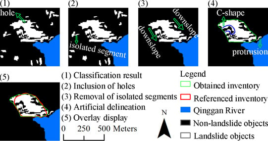
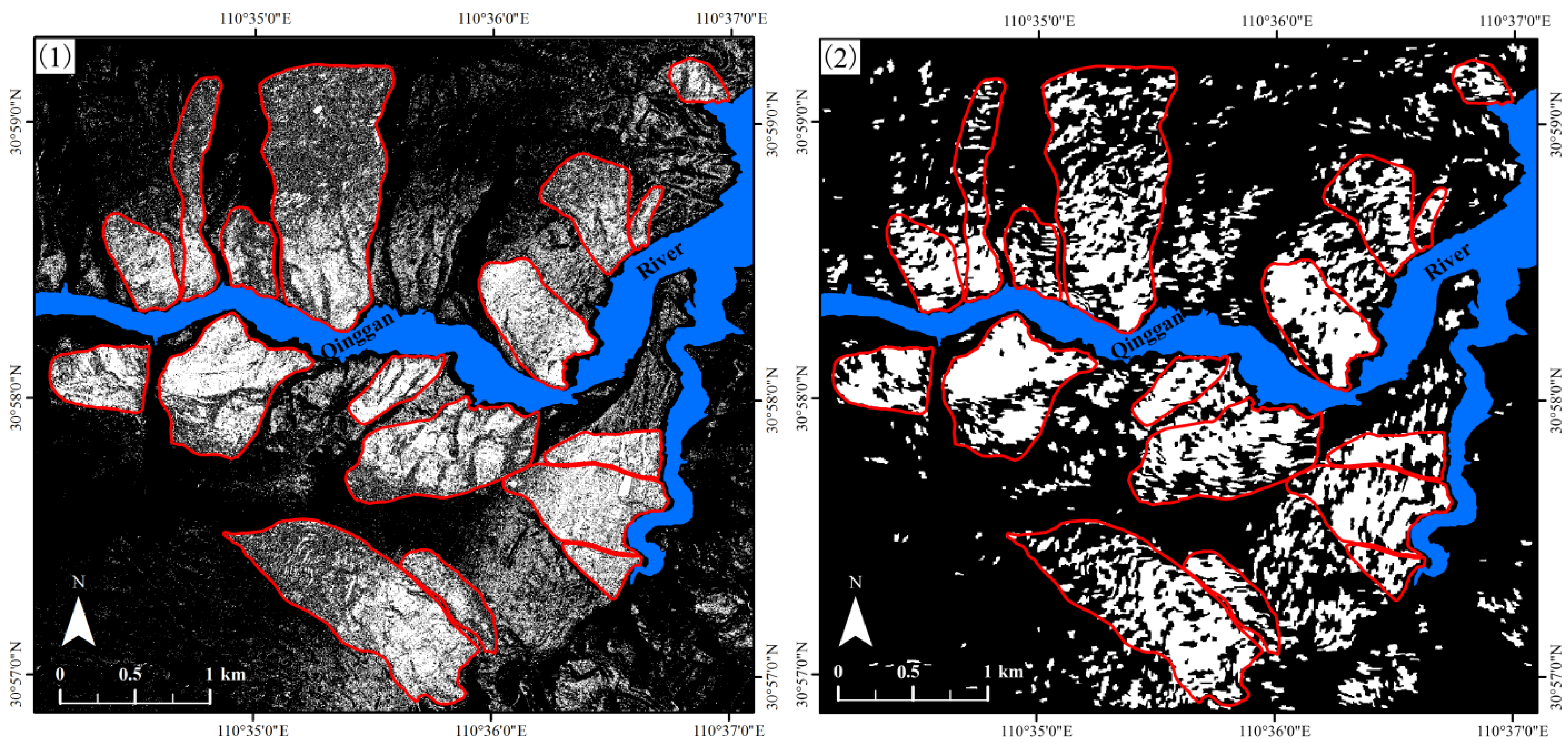
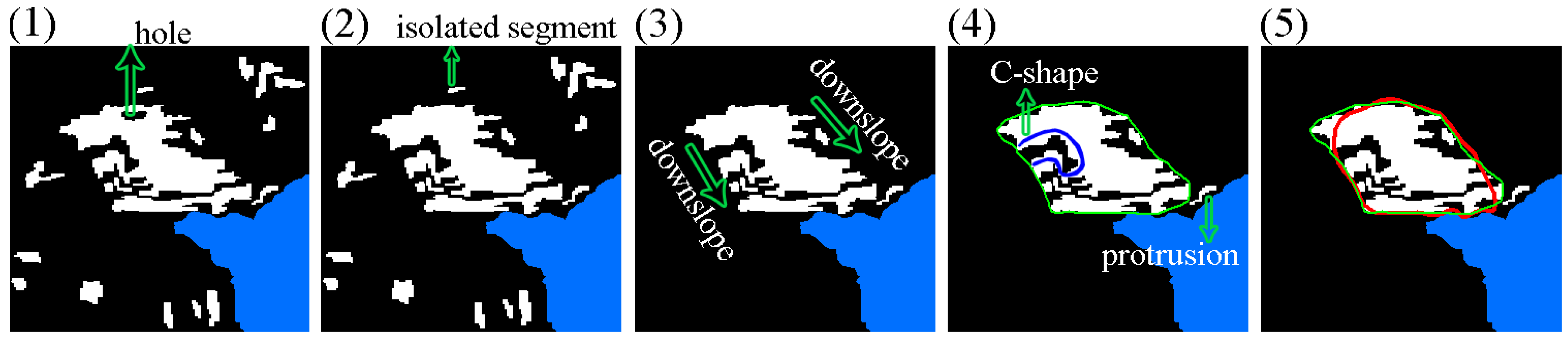
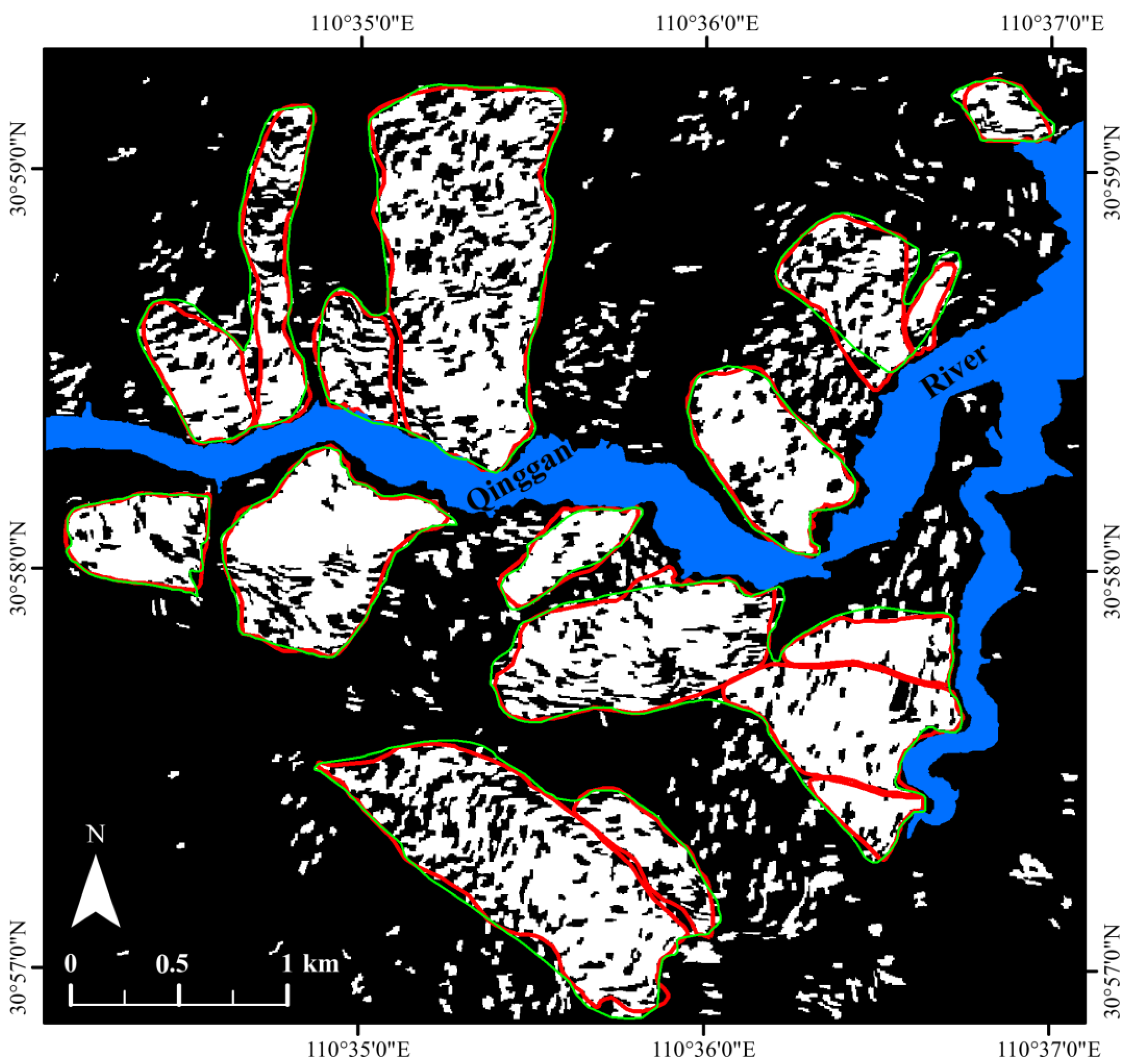
4.4. Landslide Inventory Map and Accuracy Assessment

As training sets, 50% of the OLS and ONLS were selected and, along with the features subset, were used to train the RF models. Then, the classification results of the study area were obtained, and an OA of 89.11% ± 0.03% was achieved. Based on the classification results, the landslide inventory map was finally achieved via the following steps: (1) inclusion of patches encircled by the spatially connective terrain segments classified as OLS; (2) removal of isolated and small segments that are located away from rivers and landslide bodies, and where landslide occurrence is almost impossible; and (3) delineation of closed envelope curves for OLS by manual digitizing operation using the Editor toolbar in ArcGIS software. In the first two steps, the classification result was first converted to vector polygon data, then the Editor toolbar in ArcGIS software was used to include and remove the corresponding segments, and the processed polygon data were finally converted to raster data. In step two, if the inclusion of an isolated landslide segment resulted in the destruction of the overall shape of a landslide body or made the increased non-landslide area larger than the area of the isolated segment, the isolated segment would be removed. In step three, the following guidelines should be followed: (1) the boundaries should be smooth; (2) landslide flanks must be drawn in the down-slope direction in which the displaced material moves; (3) the C-shaped half surrounding boundaries should be closed; and (4) the overall trend of the flanks should be followed, and protrusions on the flanks should be ignored. A schematic diagram for landslide identification in the upper-right corner of the study area is shown in Figure 6. The extracted inventory map is shown in Figure 7. All landslides were identified, and visual comparison indicated that the obtained inventory map agrees well with the reference landslide inventory map. Some polygons in the map consisted of multiple landslides, and therefore had strange shapes. The position mismatch (PM) [45,102] was selected to assess the obtained inventory map. PM is defined as:
P M = A R O A R O A R O × 100 %
where A R O is the area designated as a landslide either by the reference inventory or the object-based inventory, and A R O is the area designated as a landslide by both inventories, namely, the union ( ) and intersection ( ) of two maps. The PM value was 9%, demonstrating that the two inventories were essentially the same. For OBIA using topographic information, the landslide parts are represented by multiple segments, and it is difficult to aggregate these segments into one final landslide segment [39]. As a result, automated extraction of a landslide inventory map is very difficult for OBIA with only LiDar data. Compared to the delineation of landslide boundaries in the previous PBA [42], although the inventory map was artificially delineated, OBIA was able to yield a continuous result with specific physical meaning and interpretability. Because the main scarp in the study area is either indistinct or difficult to distinguish from surrounding objects, this study did not differentiate landslide parts. As a result, the delineation of the landslide inventory map in this study was simpler than that of Van den Eeckhaut et al. [39]. Van den Eeckhaut et al. [39] used a calibration area of 9.7 km2 (about 19.4% of the study area) and the obtained PM ranged between 57% and 66%. However, to make a comparison of OBIA and the previous PBA [42], this study utilized lots of training data (50% of the OLS and ONLS) so as to produce a result that was very close to the reference polygons (with a PM value of 9%).
Figure 6. Schematic diagram and main steps for extraction of a landslide inventory map in the upper-right corner of the study area. (1) Classification results. White and black patches represent objects classified as OLS and ONLS, respectively. Blue area represents the Qinggan River. (2) Inclusion of holes. (3) Removal of isolated segments. (4) Delineation of closed envelope curves for OLS by manual digitizing operation. Green solid lines represent the outlined landslide inventory map. (5) Overlay display of the extracted landslide inventory map on the referenced inventory map. Red solid lines represent the referenced inventory map.
Remotesensing 07 09705 g006
Figure 7. Extracted inventory map (green solid lines) overlayed on the referenced landslide inventory map and classification result. White patches represent objects classified as OLS, and black patches represent ONLS. Red solid lines represent the referenced inventory map.
Remotesensing 07 09705 g007

5. Conclusions

Using an OBIA method with only LiDar data, a semi-automatic forested landslide identification process was implemented in areas of dense vegetation, bedrock cover and rugged terrain, within the Three Gorges region. The object features were calculated using LiDar DTMs to derive topographic, filter, and texture features, and proved effective for landslide identification. The feature selection method can markedly reduce the numbers of object features and slightly improve the classification accuracy. The features subset-based models achieved an OA of 77.36% ± 0.13% for the RF algorithm, and an OA of 76.87% ± 0.07% for the SVM algorithm. The RF algorithm had greater classification accuracies and lower sensitivity to the feature selection process than the SVM algorithm. Compared to PBA, OBIA was more sensitive to feature selection, remarkably reduced computing time, and depicted more contiguous terrain segments that had better applicability and interpretability, with slight loss of classification accuracy. Based on the classification result with an OA of 89.11% ± 0.03%, the obtained inventory map was consistent with the referenced landslide inventory map, with a PM value of 9%. In summary, by combining object features derived from LiDar DTMs, a feature selection method, and machine learning algorithms, it was shown that the semi-automatic method is useful for forested landslide identification in steep and rugged terrain with bedrock cover. Future work will focus on other feature selection and image segmentation algorithms, image segmentation using other topographic data or aerial images, automated and objective selection of scale parameters for segmentation, DTM data with different spatial resolutions, new dataset sampling designs for feature selection and classification, automatic delineation of landslide boundaries based on supervised classification results, recognition of landslide types and components, influence of climate conditions such as rainfall on landslides, and other heterogeneous landscape areas. Also, when using randomly selected samples as training data, it is worth considering the number of required random runs and how this number will be affected by landscape or landslide type. All of these factors can help improve the transferability of the approach developed in this study.

Acknowledgments

This research was jointly supported by the Fundamental Research Funds for the Central Universities, China University of Geosciences (Wuhan) (No.CUGL150417), the China Geological Survey (No. 2010200082), the China Scholarship Council (No. 201406415051), and the Natural Science Foundation of Hubei Province of China (No.2011CDB350). The authors also thank the China Aero Geophysical Survey and Remote Sensing Center for Land and Resources for providing the LiDar data used in the study.

Author Contributions

Xianju Li and Weitao Chen conceived of, designed, and performed the experiments and wrote the manuscript. Xinwen Cheng and Gang Chen analyzed the data and revised the manuscript. Shengwei Liu helped to obtain the LiDar data.

Conflicts of Interest

The authors declare no conflict of interest.

References

  1. Bai, S.-B.; Wang, J.; Lue, G.-N.; Zhou, P.-G.; Hou, S.-S.; Xu, S.-N. GIS-based and data-driven bivariate landslide-susceptibility mapping in the Three Gorges area, China. Pedosphere 2009, 19, 14–20. [Google Scholar] [CrossRef]
  2. Bai, S.-B.; Wang, J.; Lue, G.-N.; Zhou, P.-G.; Hou, S.-S.; Xu, S.-N. GIS-based logistic regression for landslide susceptibility mapping of the Zhongxian segment in the Three Gorges area, China. Geomorphology 2010, 115, 23–31. [Google Scholar] [CrossRef]
  3. Liu, J.G.; Mason, P.J.; Clerici, N.; Chen, S.; Davis, A.; Miao, F.; Deng, H.; Liang, L. Landslide hazard assessment in the Three Gorges area of the Yangtze River using aster imagery: Zigui-badong. Geomorphology 2004, 61, 171–187. [Google Scholar] [CrossRef]
  4. Ni, J.; Shao, J.A. The drivers of land use change in the migration area, Three Gorges project, China: Advances and prospects. J. Earth Sci. 2013, 24, 136–144. [Google Scholar] [CrossRef]
  5. Akgun, A.; Dag, S.; Bulut, F. Landslide susceptibility mapping for a landslide-prone area (Findikli, NE of Turkey) by likelihood-frequency ratio and weighted linear combination models. Environ. Geol. 2008, 54, 1127–1143. [Google Scholar] [CrossRef]
  6. Ardizzone, F.; Cardinali, M.; Galli, M.; Guzzetti, F.; Reichenbach, P. Identification and mapping of recent rainfall-induced landslides using elevation data collected by airborne LiDar. Nat. Hazards Earth Syst. Sci. 2007, 7, 637–650. [Google Scholar] [CrossRef]
  7. Constantin, M.; Bednarik, M.; Jurchescu, M.C.; Vlaicu, M. Landslide susceptibility assessment using the bivariate statistical analysis and the index of entropy in the Sibiciu basin (Romania). Environ. Earth Sci. 2011, 63, 397–406. [Google Scholar] [CrossRef]
  8. Fiorucci, F.; Cardinali, M.; Carla, R.; Rossi, M.; Mondini, A.C.; Santurri, L.; Ardizzone, F.; Guzzetti, F. Seasonal landslide mapping and estimation of landslide mobilization rates using aerial and satellite images. Geomorphology 2011, 129, 59–70. [Google Scholar] [CrossRef]
  9. Guzzetti, F.; Mondini, A.C.; Cardinali, M.; Fiorucci, F.; Santangelo, M.; Chang, K.-T. Landslide inventory maps: New tools for an old problem. Earth Sci. Rev. 2012, 112, 42–66. [Google Scholar] [CrossRef]
  10. Thiery, Y.; Malet, J.P.; Sterlacchini, S.; Puissant, A.; Maquaire, O. Landslide susceptibility assessment by bivariate methods at large scales: Application to a complex mountainous environment. Geomorphology 2007, 92, 38–59. [Google Scholar] [CrossRef] [Green Version]
  11. Van Westen, C.J.; Castellanos, E.; Kuriakose, S.L. Spatial data for landslide susceptibility, hazard, and vulnerability assessment: An overview. Eng. Geol. 2008, 102, 112–131. [Google Scholar] [CrossRef]
  12. McKean, J.; Roering, J. Objective landslide detection and surface morphology mapping using high-resolution airborne laser altimetry. Geomorphology 2004, 57, 331–351. [Google Scholar] [CrossRef]
  13. Wills, C.J.; McCrink, T.P. Comparing landslide inventories: The map depends on the method. Environ. Eng. Geosci. 2002, 8, 279–293. [Google Scholar] [CrossRef]
  14. Barlow, J.; Franklin, S.; Martin, Y. High spatial resolution satellite imagery, DEM derivatives, and image segmentation for the detection of mass wasting processes. Photogramm. Eng. Remote Sens. 2006, 72, 687–692. [Google Scholar] [CrossRef]
  15. Behling, R.; Roessner, S.; Kaufmann, H.; Kleinschmit, B. Automated spatiotemporal landslide mapping over large areas using rapideye time series data. Remote Sens. 2014, 6, 8026–8055. [Google Scholar] [CrossRef]
  16. Bianchini, S.; Herrera, G.; Maria Mateos, R.; Notti, D.; Garcia, I.; Mora, O.; Moretti, S. Landslide activity maps generation by means of persistent scatterer interferometry. Remote Sens. 2013, 5, 6198–6222. [Google Scholar] [CrossRef]
  17. Borghuis, A.M.; Chang, K.; Lee, H.Y. Comparison between automated and manual mapping of typhoon-triggered landslides from SPOT-5 imagery. Int. J. Remote Sens. 2007, 28, 1843–1856. [Google Scholar] [CrossRef]
  18. Guzzetti, F.; Cardinali, M.; Reichenbach, P.; Carrara, A. Comparing landslide maps: A case study in the upper Tiber River basin, central Italy. Environ. Manag. 2000, 25, 247–263. [Google Scholar] [CrossRef]
  19. Lacroix, P.; Zavala, B.; Berthier, E.; Audin, L. Supervised method of landslide inventory using panchromatic SPOT-5 images and application to the earthquake-triggered landslides of Pisco (Peru, 2007, MW8.0). Remote Sens. 2013, 5, 2590–2616. [Google Scholar] [CrossRef] [Green Version]
  20. Lu, P.; Stumpf, A.; Kerle, N.; Casagli, N. Object-oriented change detection for landslide rapid mapping. IEEE Geosci. Remote Sens. Lett. 2011, 8, 701–705. [Google Scholar] [CrossRef]
  21. Lu, P.; Bai, S.; Casagli, N. Investigating spatial patterns of persistent scatterer interferometry point targets and landslide occurrences in the Arno River basin. Remote Sens. 2014, 6, 6817–6843. [Google Scholar] [CrossRef]
  22. Martha, T.R.; Kerle, N.; Jetten, V.; van Westen, C.J.; Kumar, K.V. Characterising spectral, spatial and morphometric properties of landslides for semi-automatic detection using object-oriented methods. Geomorphology 2010, 116, 24–36. [Google Scholar] [CrossRef]
  23. Metternicht, G.; Hurni, L.; Gogu, R. Remote sensing of landslides: An analysis of the potential contribution to geo-spatial systems for hazard assessment in mountainous environments. Remote Sens. Environ. 2005, 98, 284–303. [Google Scholar] [CrossRef]
  24. Nichol, J.; Wong, M.S. Satellite remote sensing for detailed landslide inventories using change detection and image fusion. Int. J. Remote Sens. 2005, 26, 1913–1926. [Google Scholar] [CrossRef]
  25. Rau, J.-Y.; Chen, L.-C.; Liu, J.-K.; Wu, T.-H. Dynamics monitoring and disaster assessment for watershed management using time-series satellite images. IEEE Trans. Geosci. Remote Sens. 2007, 45, 1641–1649. [Google Scholar] [CrossRef]
  26. Scaioni, M. Remote sensing for landslide investigations: From research into practice. Remote Sens. 2013, 5, 5488–5492. [Google Scholar] [CrossRef]
  27. Scaioni, M.; Longoni, L.; Melillo, V.; Papini, M. Remote sensing for landslide investigations: An overview of recent achievements and perspectives. Remote Sens. 2014, 6, 9600–9652. [Google Scholar] [CrossRef]
  28. Stumpf, A.; Kerle, N. Object-oriented mapping of landslides using random forests. Remote Sens. Environ. 2011, 115, 2564–2577. [Google Scholar] [CrossRef]
  29. Van den Eeckhaut, M.; Poesen, J.; Verstraeten, G.; Vanacker, V.; Moeyersons, J.; Nyssen, J.; van Beek, L.P.H. The effectiveness of hillshade maps and expert knowledge in mapping old deep-seated landslides. Geomorphology 2005, 67, 351–363. [Google Scholar] [CrossRef]
  30. Whitworth, M.C.Z.; Giles, D.P.; Murphy, W. Airborne remote sensing for landslide hazard assessment: A case study on the jurassic escarpment slopes of Worcestershire, UK. Q. J. Eng. Geol. Hydrogeol. 2005, 38, 285–300. [Google Scholar] [CrossRef]
  31. Borkowski, A.; Perski, Z.; Wojciechowski, T.; Jozkow, G.; Wojcik, A. Landslides mapping in Roznow Lake vicinity, Poland using airborne laser scanning data. Acta Geodyn. Geomater. 2011, 8, 325–333. [Google Scholar]
  32. Haneberg, W.C.; Cole, W.F.; Kasali, G. High-resolution LiDar-based landslide hazard mapping and modeling, UCSF Parnassus Campus, San Francisco, USA. Bull. Eng. Geol. Environ. 2009, 68, 263–276. [Google Scholar] [CrossRef]
  33. Jaboyedoff, M.; Oppikofer, T.; Abellan, A.; Derron, M.-H.; Loye, A.; Metzger, R.; Pedrazzini, A. Use of LiDar in landslide investigations: A review. Nat. Hazards 2012, 61, 5–28. [Google Scholar] [CrossRef]
  34. Kasai, M.; Ikeda, M.; Asahina, T.; Fujisawa, K. LiDar-derived DEM evaluation of deep-seated landslides in a steep and rocky region of Japan. Geomorphology 2009, 113, 57–69. [Google Scholar] [CrossRef]
  35. Lin, C.-W.; Tseng, C.-M.; Tseng, Y.-H.; Fei, L.-Y.; Hsieh, Y.-C.; Tarolli, P. Recognition of large scale deep-seated landslides in forest areas of Taiwan using high resolution topography. J. Asian Earth Sci. 2013, 62, 389–400. [Google Scholar] [CrossRef]
  36. Lin, M.-L.; Chen, T.-W.; Lin, C.-W.; Ho, D.-J.; Cheng, K.-P.; Yin, H.-Y.; Chen, M.-C. Detecting large-scale landslides using LiDar data and aerial photos in the Namasha-Liuoguey area, Taiwan. Remote Sens. 2014, 6, 42–63. [Google Scholar] [CrossRef]
  37. Liu, J.-K.; Hsiao, K.-H.; Shih, P.T.-Y. A geomorphological model for landslide detection using airborne LiDar data. J. Mar. Sci. Technol. Taiwan 2012, 20, 629–638. [Google Scholar]
  38. Rau, J.-Y.; Chang, K.-T.; Shao, Y.-C.; Lau, C.-C. Semi-automatic shallow landslide detection by the integration of airborne imagery and laser scanning data. Nat. Hazards 2012, 61, 469–480. [Google Scholar] [CrossRef]
  39. Van den Eeckhaut, M.; Kerle, N.; Poesen, J.; Hervas, J. Object-oriented identification of forested landslides with derivatives of single pulse LiDar data. Geomorphology 2012, 173, 30–42. [Google Scholar] [CrossRef]
  40. Wang, G.; Joyce, J.; Phillips, D.; Shrestha, R.; Carter, W. Delineating and defining the boundaries of an active landslide in the rainforest of puerto rico using a combination of airborne and terrestrial LiDar data. Landslides 2013, 10, 503–513. [Google Scholar] [CrossRef]
  41. Booth, A.M.; Roering, J.J.; Perron, J.T. Automated landslide mapping using spectral analysis and high-resolution topographic data: Puget sound lowlands, washington, and Portland hills, Oregon. Geomorphology 2009, 109, 132–147. [Google Scholar] [CrossRef]
  42. Chen, W.; Li, X.; Wang, Y.; Chen, G.; Liu, S. Forested landslide detection using LiDar data and the random forest algorithm: A case study of the Three Gorges, China. Remote Sens. Environ. 2014, 152, 291–301. [Google Scholar] [CrossRef]
  43. Glenn, N.F.; Streutker, D.R.; Chadwick, D.J.; Thackray, G.D.; Dorsch, S.J. Analysis of LiDar-derived topographic information for characterizing and differentiating landslide morphology and activity. Geomorphology 2006, 73, 131–148. [Google Scholar] [CrossRef]
  44. Schulz, W.H. Landslide susceptibility revealed by LiDar imagery and historical records, Seattle, Washington. Eng. Geol. 2007, 89, 67–87. [Google Scholar] [CrossRef]
  45. Van den Eeckhaut, M.; Poesen, J.; Verstraeten, G.; Vanacker, V.; Nyssen, J.; Moeyersons, J.; van Beek, L.P.H.; Vandekerckhove, L. Use of LiDar-derived images for mapping old landslides under forest. Earth Surf. Process. Landf. 2007, 32, 754–769. [Google Scholar] [CrossRef]
  46. Van den Eeckhaut, M.; Moeyersons, J.; Nyssen, J.; Abraha, A.; Poesen, J.; Haile, M.; Deckers, J. Spatial patterns of old, deep-seated landslides: A case-study in the Northern Ethiopian Highlands. Geomorphology 2009, 105, 239–252. [Google Scholar] [CrossRef]
  47. Van den Eeckhaut, M.; Poesen, J.; Gullentops, F.; Vandekerckhove, L.; Hervas, J. Regional mapping and characterisation of old landslides in hilly regions using LiDar-based imagery in southern Flanders. Quat. Res. 2011, 75, 721–733. [Google Scholar] [CrossRef]
  48. Blaschke, T. Object based image analysis for remote sensing. ISPRS J. Photogramm. Remote Sens. 2010, 65, 2–16. [Google Scholar] [CrossRef]
  49. Duro, D.C.; Franklin, S.E.; Dube, M.G. Multi-scale object-based image analysis and feature selection of multi-sensor earth observation imagery using random forests. Int. J. Remote Sens. 2012, 33, 4502–4526. [Google Scholar] [CrossRef]
  50. Barlow, J.; Martin, Y.; Franklin, S.E. Detecting translational landslide scars using segmentation of landsat ETM+ and DEM data in the northern Cascade Mountains, British Columbia. Can. J. Remote Sens. 2003, 29, 510–517. [Google Scholar] [CrossRef]
  51. Martha, T.R.; Kerle, N.; van Westen, C.J.; Jetten, V.; Kumar, K.V. Segment optimization and data-driven thresholding for knowledge-based landslide detection by object-based image analysis. IEEE Trans. Geosci. Remote Sens. 2011, 49, 4928–4943. [Google Scholar] [CrossRef]
  52. Martha, T.R.; Kerle, N.; van Westen, C.J.; Jetten, V.; Kumar, K.V. Object-oriented analysis of multi-temporal panchromatic images for creation of historical landslide inventories. ISPRS J. Photogramm. Remote Sens. 2012, 67, 105–119. [Google Scholar] [CrossRef]
  53. Anders, N.S.; Seijmonsbergen, A.C.; Bouten, W. Geomorphological change detection using object-based feature extraction from multi-temporal LiDar data. IEEE Geosci. Remote Sens. Lett. 2013, 10, 1587–1591. [Google Scholar] [CrossRef]
  54. Eisank, C.; Smith, M.; Hillier, J. Assessment of multiresolution segmentation for delimiting drumlins in digital elevation models. Geomorphology 2014, 214, 452–464. [Google Scholar] [CrossRef] [PubMed]
  55. Chen, W.; Li, X.; Wang, Y.; Liu, S. Landslide susceptibility mapping using LiDar and DMC data: A case study in the Three Gorges area, China. Environ. Earth Sci. 2013, 70, 673–685. [Google Scholar] [CrossRef]
  56. Chen, G.; Li, X.; Chen, W.; Cheng, X.; Zhang, Y.; Liu, S. Extraction and application analysis of landslide influential factors based on LiDar dem: A case study in the Three Gorges area, China. Nat. Hazards 2014, 74, 509–526. [Google Scholar] [CrossRef]
  57. Ladha, L.; Deepa, T. Feature selection methods and algorithms. Int. J. Comp. Sci. Eng. 2011, 3, 1787–1797. [Google Scholar]
  58. ARC/INFO China Technical Advice and Training Center. Arc/info GIS Application Tutorial: Grid and Tin; ERSI China: Beijing, China, 1995. (In Chinese) [Google Scholar]
  59. Addink, E.A.; de Jong, S.M.; Pebesma, E.J. The importance of scale in object-based mapping of vegetation parameters with hyperspectral imagery. Photogramm. Eng. Remote Sens. 2007, 73, 905–912. [Google Scholar] [CrossRef]
  60. Myint, S.W.; Gober, P.; Brazel, A.; Grossman-Clarke, S.; Weng, Q. Per-pixel vs. object-based classification of urban land cover extraction using high spatial resolution imagery. Remote Sens. Environ. 2011, 115, 1145–1161. [Google Scholar] [CrossRef]
  61. Baatz, M.; Schäpe, A. Multiresolution segmentation: An optimization approach for high quality multi-scale image segmentation. In Angewandte Geographische Informationsverarbeitung XII; Strobl, J., Blaschke, T., Griesebner, G., Eds.; Wichmann Verlag: Karlsruhe, Germany, 2000; pp. 12–23. [Google Scholar]
  62. Dragut, L.; Csillik, O.; Eisank, C.; Tiede, D. Automated parameterisation for multi-scale image segmentation on multiple layers. ISPRS J. Photogramm. Remote Sens. 2014, 88, 119–127. [Google Scholar] [CrossRef] [PubMed]
  63. Benz, U.C.; Hofmann, P.; Willhauck, G.; Lingenfelder, I.; Heynen, M. Multi-resolution, object-oriented fuzzy analysis of remote sensing data for GIS-ready information. ISPRS J. Photogramm. Remote Sens. 2004, 58, 239–258. [Google Scholar] [CrossRef]
  64. Gao, Y.; Francois Mas, J.; Kerle, N.; Navarrete Pacheco, J.A. Optimal region growing segmentation and its effect on classification accuracy. Int. J. Remote Sens. 2011, 32, 3747–3763. [Google Scholar] [CrossRef]
  65. Liu, D.; Xia, F. Assessing object-based classification: Advantages and limitations. Remote Sens. Lett. 2010, 1, 187–194. [Google Scholar] [CrossRef]
  66. Smith, A. Image segmentation scale parameter optimization and land cover classification using the random forest algorithm. J. Spat. Sci. 2010, 55, 69–79. [Google Scholar] [CrossRef]
  67. Kim, M.; Warner, T.A.; Madden, M.; Atkinson, D.S. Multi-scale GEOBIA with very high spatial resolution digital aerial imagery: Scale, texture and image objects. Int. J. Remote Sens. 2011, 32, 2825–2850. [Google Scholar] [CrossRef]
  68. Dragut, L.; Tiede, D.; Levick, S.R. ESP: A tool to estimate scale parameter for multiresolution image segmentation of remotely sensed data. Int. J. Geogr. Inf. Sci. 2010, 24, 859–871. [Google Scholar] [CrossRef]
  69. Dragut, L.; Eisank, C. Automated object-based classification of topography from SRTM data. Geomorphology 2012, 141, 21–33. [Google Scholar] [CrossRef] [PubMed]
  70. Espindola, G.M.; Camara, G.; Reis, I.A.; Bins, L.S.; Monteiro, A.M. Parameter selection for region-growing image segmentation algorithms using spatial autocorrelation. Int. J. Remote Sens. 2006, 27, 3035–3040. [Google Scholar] [CrossRef]
  71. Johnson, B.; Xie, Z. Unsupervised image segmentation evaluation and refinement using a multi-scale approach. ISPRS J. Photogramm. Remote Sens. 2011, 66, 473–483. [Google Scholar] [CrossRef]
  72. Zhang, H.; Fritts, J.E.; Goldman, S.A. Image segmentation evaluation: A survey of unsupervised methods. Comput. Vis. Image Underst. 2008, 110, 260–280. [Google Scholar] [CrossRef]
  73. Duro, D.C.; Franklin, S.E.; Dube, M.G. A comparison of pixel-based and object-based image analysis with selected machine learning algorithms for the classification of agricultural landscapes using SPOT-5 HRG imagery. Remote Sens. Environ. 2012, 118, 259–272. [Google Scholar] [CrossRef]
  74. Robertson, L.D.; King, D.J. Comparison of pixel- and object-based classification in land cover change mapping. Int. J. Remote Sens. 2011, 32, 1505–1529. [Google Scholar] [CrossRef]
  75. Laliberte, A.S.; Fredrickson, E.L.; Rango, A. Combining decision trees with hierarchical object-oriented image analysis for mapping arid rangelands. Photogram. Eng. Remote Sens. 2007, 73, 197–207. [Google Scholar] [CrossRef]
  76. Mathieu, R.; Aryal, J.; Chong, A.K. Object-based classification of IKONOS imagery for mapping large-scale vegetation communities in urban areas. Sensors 2007, 7, 2860–2880. [Google Scholar] [CrossRef]
  77. Pu, R.; Landry, S.; Yu, Q. Object-based urban detailed land cover classification with high spatial resolution IKONOS imagery. Int. J. Remote Sens. 2011, 32, 3285–3308. [Google Scholar] [CrossRef]
  78. Whiteside, T.G.; Boggs, G.S.; Maier, S.W. Comparing object-based and pixel-based classifications for mapping savannas. Int. J. Appl. Earth Obs. Geoinf. 2011, 13, 884–893. [Google Scholar] [CrossRef]
  79. Di, K.; Yue, Z.; Liu, Z.; Wang, S. Automated rock detection and shape analysis from Mars rover imagery and 3D point cloud data. J. Earth Sci. 2013, 24, 125–135. [Google Scholar] [CrossRef]
  80. eCognition. Ecognition Developer 8.0.1 User Guide; Document Version 1.2.1; Definiens AG: Munich, Germany, 2010. [Google Scholar]
  81. Fernandez Galarreta, J.; Kerle, N.; Gerke, M. UAV-based urban structural damage assessment using object-based image analysis and semantic reasoning. Nat. Hazards Earth Syst. Sci. 2015, 15, 1087–1101. [Google Scholar] [CrossRef]
  82. Fernandez Galarreta, J. Urban Structural Damage Assessment Using Object-Oriented Analysis and Semantic Reasoning. Master’s Thesis, University of Twente, Enschede, Netherlands, 2014. [Google Scholar]
  83. Chan, J.C.-W.; Paelinckx, D. Evaluation of random forest and adaboost tree-based ensemble classification and spectral band selection for ecotope mapping using airborne hyperspectral imagery. Remote Sens. Environ. 2008, 112, 2999–3011. [Google Scholar] [CrossRef]
  84. Genuer, R.; Poggi, J.-M.; Tuleau-Malot, C. Variable selection using random forests. Pattern Recognit. Lett. 2010, 31, 2225–2236. [Google Scholar] [CrossRef]
  85. Van Coillie, F.M.B.; Verbeke, L.P.C.; de Wulf, R.R. Feature selection by genetic algorithms in object-based classification of IKONOS imagery for forest mapping in Flanders, Belgium. Remote Sens. Environ. 2007, 110, 476–487. [Google Scholar] [CrossRef]
  86. Yu, Q.; Gong, P.; Clinton, N.; Biging, G.; Kelly, M.; Schirokauer, D. Object-based detailed vegetation classification. With airborne high spatial resolution remote sensing imagery. Photogram. Eng. Remote Sens. 2006, 72, 799–811. [Google Scholar] [CrossRef]
  87. Martha, T.R. Detection of Landslides by Object-oriented Image Analysis. Ph.D. Thesis, University of Twente, Enschede, The Netherlands, 2011. [Google Scholar]
  88. Diaz-Uriarte, R. Varselrf: Variable Selection Using Random Forests; R Package Version 0.7–3; TU Wien: Vienna, Austria, 2010. [Google Scholar]
  89. R Development Core Team. R: A Language and Environment for Statistical Computing; R Foundation for Statistical Computing: Vienna, Austria, 2013. [Google Scholar]
  90. Diaz-Uriarte, R.; de Andres, S.A. Gene selection and classification of microarray data using random forest. BMC Bioinform. 2006, 7. [Google Scholar] [CrossRef] [PubMed]
  91. Breiman, L. Random forests. Mach. Learn. 2001, 45, 5–32. [Google Scholar] [CrossRef]
  92. Gislason, P.O.; Benediktsson, J.A.; Sveinsson, J.R. Random forests for land cover classification. Pattern Recognit. Lett. 2006, 27, 294–300. [Google Scholar] [CrossRef]
  93. Lawrence, R.L.; Wood, S.D.; Sheley, R.L. Mapping invasive plants using hyperspectral imagery and Breiman Cutler classifications (RandomForest). Remote Sens. Environ. 2006, 100, 356–362. [Google Scholar] [CrossRef]
  94. Watts, J.D.; Lawrence, R.L.; Miller, P.R.; Montagne, C. Monitoring of cropland practices for carbon sequestration purposes in north central Montana by landsat remote sensing. Remote Sens. Environ. 2009, 113, 1843–1852. [Google Scholar] [CrossRef]
  95. Liaw, A.; Wiener, M. Classification and regression by RandomForest. R News 2002, 2, 18–22. [Google Scholar]
  96. Vapnik, V. The Nature of Statistical Learning Theory; Springer-Verlag, Inc.: New York, NY, USA, 1995. [Google Scholar]
  97. Chang, K.-T.; Liu, J.-K.; Wang, C.-I. An object-oriented analysis for characterizing the rainfall-induced shallow landslide. J. Mar. Sci. Technol. Taiwan 2012, 20, 647–656. [Google Scholar]
  98. Peng, L.; Niu, R.; Huang, B.; Wu, X.; Zhao, Y.; Ye, R. Landslide susceptibility mapping based on rough set theory and support vector machines: A case of the Three Gorges area, China. Geomorphology 2014, 204, 287–301. [Google Scholar] [CrossRef]
  99. Meyer, D.; Dimitriadou, E.; Hornik, K.; Weingessel, A.; Leisch, F. E1071: Misc Functions of the Department of Statistics (e1071); R Package Version 1.6–4; TU Wien: Vienna, Austria, 2014. [Google Scholar]
  100. Dorren, L.K.A.; Maier, B.; Seijmonsbergen, A.C. Improved Landsat-based forest mapping in steep mountainous terrain using object-based classification. For. Ecol. Manag. 2003, 183, 31–46. [Google Scholar] [CrossRef]
  101. Stuckens, J.; Coppin, P.R.; Bauer, M.E. Integrating contextual information with per-pixel classification for improved land cover classification. Remote Sens. Environ. 2000, 71, 282–296. [Google Scholar] [CrossRef]
  102. Carrara, A.; Cardinali, M.; Detti, R.; Guzzetti, F.; Pasqui, V.; Reichenbach, P. GIS techniques and statistical-models in evaluating landslide hazard. Earth Surf. Process. Landf. 1991, 16, 427–445. [Google Scholar] [CrossRef]

