
Fodder Biomass Monitoring in Sahelian Rangelands Using Phenological Metrics from FAPAR Time Series

 , ,
, ,  ,
,
Abstract
:
1. Introduction
2. Materials and Methods
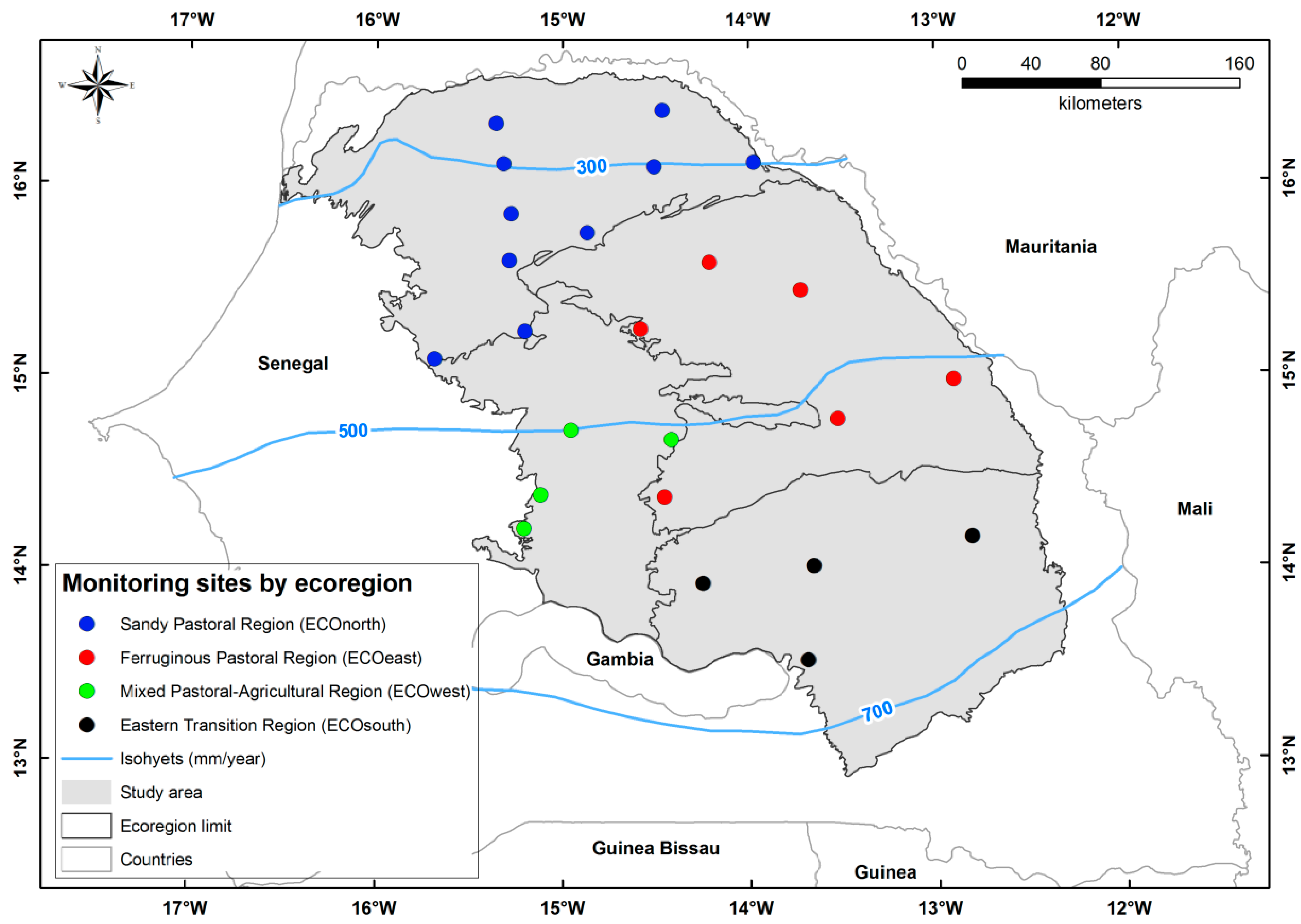
2.1. Study Area and Ground Control Sites

2.2. Biomass Data Collection

| Ecoregion | Main Vegetation Type and Woody Species | Annual Rainfall (mm) | Woody Leaf Biomass (kg·DM/ha) | Herbaceous Biomass (kg·DM/ha) | Woody Cover (%) |
|---|---|---|---|---|---|
| ECOnorth (Sandy Pastoral) | Pseudo-steppe: Boscia senegalensis, Balanites aegyptiaca, Guiera senegalensis, Calotropis procera, Combretum glutinosum, Sclerocarya birrea | 345 | 490 | 905 | 5.5 |
| ECOeast (Ferruginous Pastoral) | Shrub savannah: G. senegalensis, C. glutinosum, Pterocarpus lucens, Grewia bicolor, B. senegalensis, Adenium obesum | 488 | 1219 | 1257 | 17.7 |
| ECOwest (Pastoral-Agricultural) | Shrub/tree savannah: C. glutinosum, G. senegalensis, G. bicolor, B. senegalensis, C. micranthum, Commiphora africana | 524 | 1204 | 1867 | 16.9 |
| ECOsouth (Eastern Transition) | Tree savannah/woodland: C. glutinosum, Strychnos spinosa, Acacia macrostachya, Crossopteryx febrifuga, Terminalia avicennioides, Maytenus senegalensis | 633 | 2611 | 1937 | 33.1 |
2.2.1. Herbaceous Biomass Collection
2.2.2. Woody Leaf Biomass Collection
2.2.3. Filtering the Ground Dataset
2.3. Satellite Data
2.3.1. CSE Biomass Product
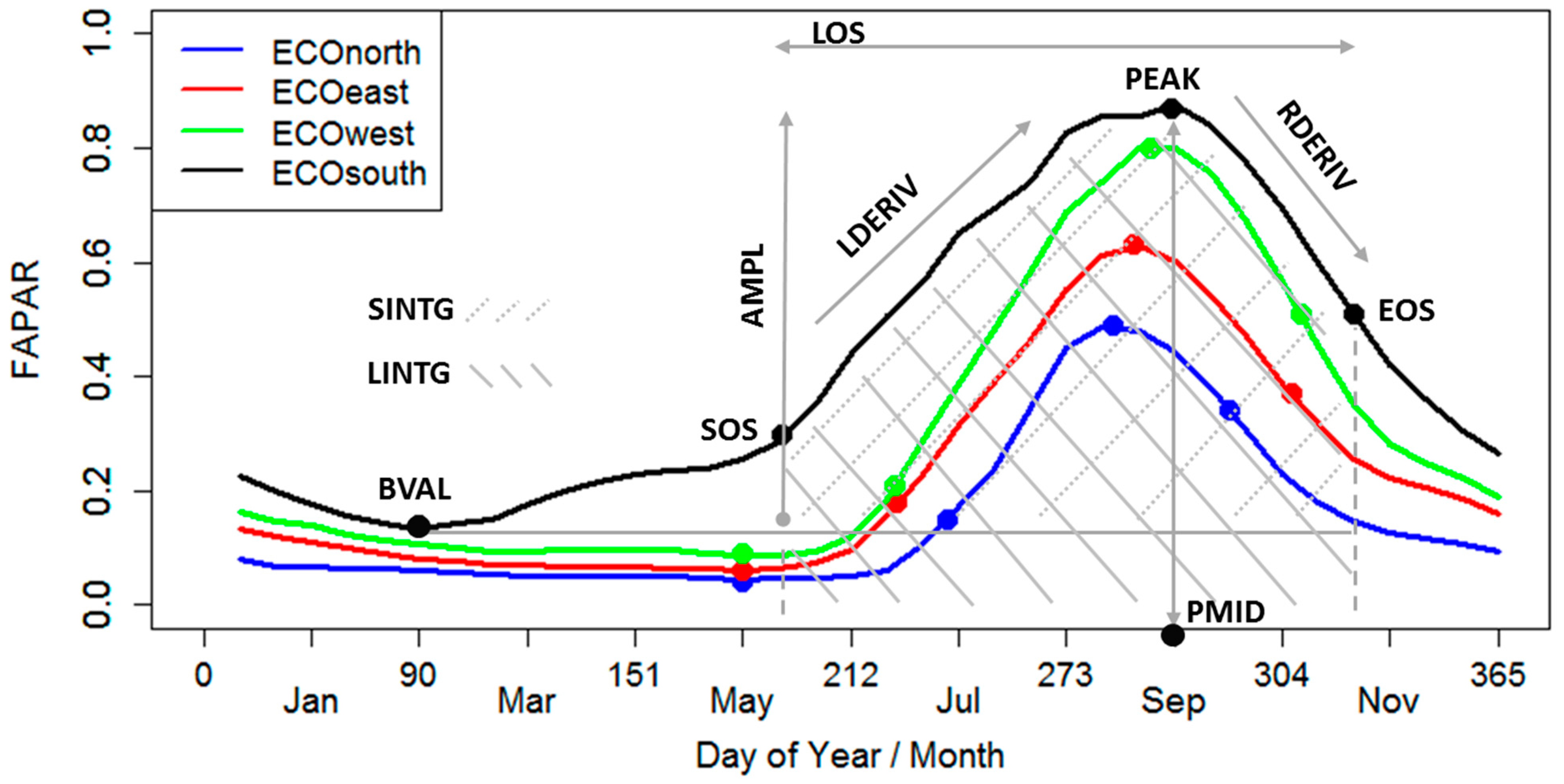
2.3.2. Phenological Metrics from FAPAR Time Series
| No. | Variables | Abbreviation | Short Definition |
|---|---|---|---|
| 1 | Start of season | SOS | Time when the left edge has increased to 20% of the amplitude |
| 2 | End of season | EOS | Time when the right edge has decreased to 50% of the amplitude |
| 3 | Length of season | LOS | Time from the SOS to the EOS |
| 4 | Middle of season | PMID | Computed as the mean value of the times when the signal is higher than 80% of the amplitude |
| 5 | Base value | BVAL | Averaged minimum values over the annual cycle |
| 6 | Maximum value | PEAK | Highest FAPAR value over the season |
| 7 | Amplitude | AMPL | Difference between the maximum and BVAL |
| 8 | Large seasonal integral | LINTG | Integral of the signal from the SOS to the EOS |
| 9 | Small seasonal integral | SINTG | Integral of the signal above the BVAL from the SOS to the EOS |
| 10 | Left derivative | LDERIV | Rate of increase at the SOS between the left 20% and 80% of the amplitude |
| 11 | Right derivative | RDERIV | Rate of decrease at the EOS between the right 20% and 80% of the amplitude |

2.4. Modeling Total Biomass Production
2.4.1. Reduction of Explanatory Variables and Model Development
| Criterion | Annotation | Formula | Decision Rule |
|---|---|---|---|
| Ajusted coefficient of determination | Adj. R2 | Performance increases with |Adj. R2| | |
| Akaike Information Criterion | AIC | n.log + 2(p+1) | Performance increases with lower AIC |
| Variation Inflation Factor | VIF | VIF > 10 points to co-linearity | |
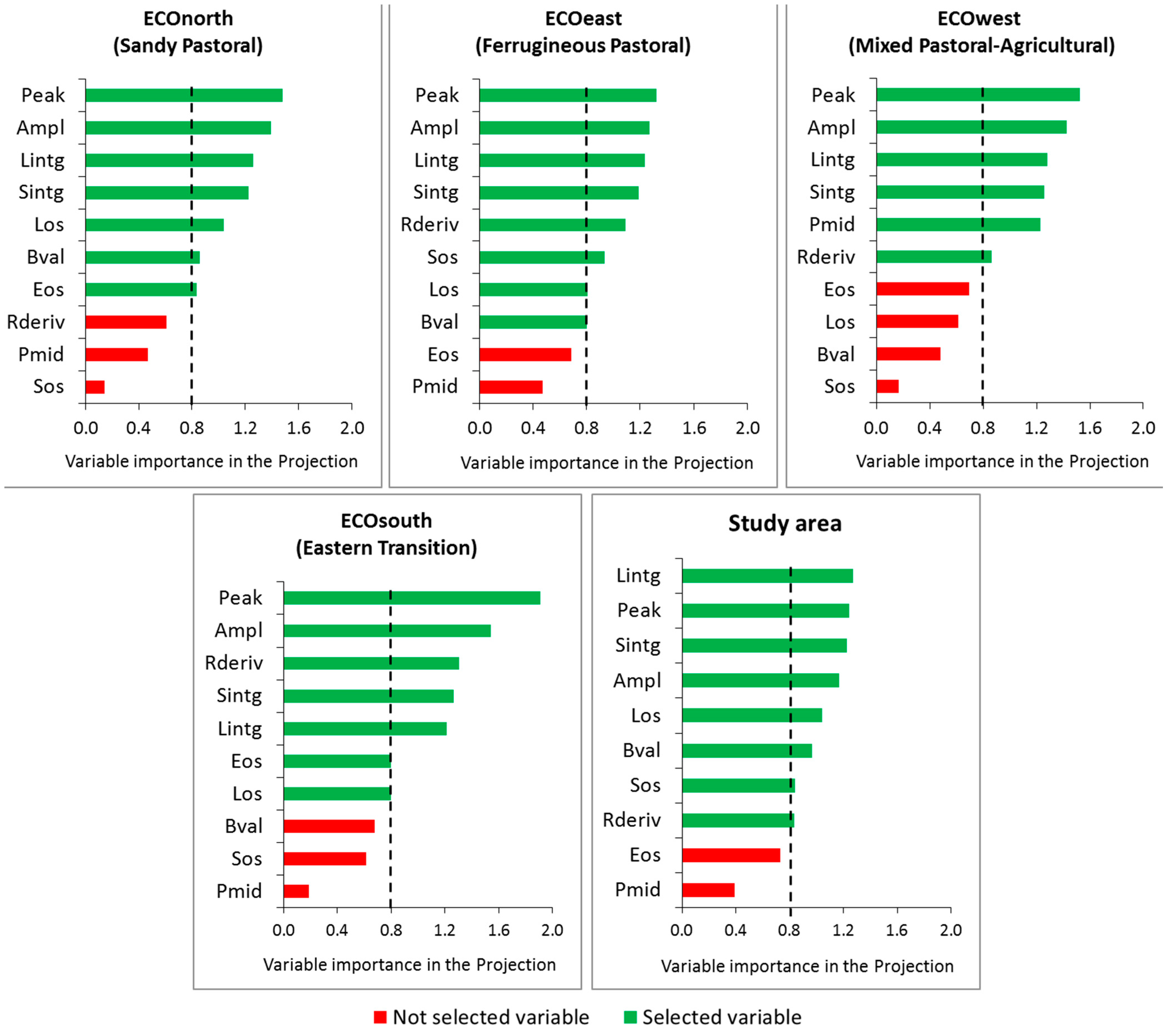
| Variable Importance in the projection | VIP | Variable is important if VIP ≥ 0.8 | |
| Mean Absolute Error | MAE | A low MAE shows higher reliability | |
| Normalized Mean Absolute Error | NMAE | A low NMAE shows higher reliability |
2.4.2. Bootstrap Resampling and Model Verification
| Variable | Simple Statistics | Pearson Correlation Statistics | ||
|---|---|---|---|---|
| Mean | SD | R | p-value | |
| LINTG | 6.09 | 2.88 | 0.79 | <0.0001 |
| PEAK | 0.65 | 0.19 | 0.77 | <0.0001 |
| SINTG | 5.25 | 2.34 | 0.76 | <0.0001 |
| AMPL | 0.59 | 0.17 | 0.72 | <0.0001 |
| LOS | 109 | 30 | 0.63 | <0.0001 |
| BVAL | 0.06 | 0.05 | 0.59 | <0.0001 |
| SOS | 196 | 20 | −0.52 | <0.0001 |
| RDERIV | 14.03 | 6.10 | 0.45 | <0.0001 |
| EOS | 304 | 21 | 0.38 | <0.0001 |
| PMID | 258 | 14 | 0.23 | 0.0002 |
| LDERIV | 20.85 | 6.21 | −0.11 | 0.0825 |
3. Results
3.1. Relationship between Total Biomass and Phenological Variables
3.2. Importance of the Explanatory Variables in Total Biomass Prediction

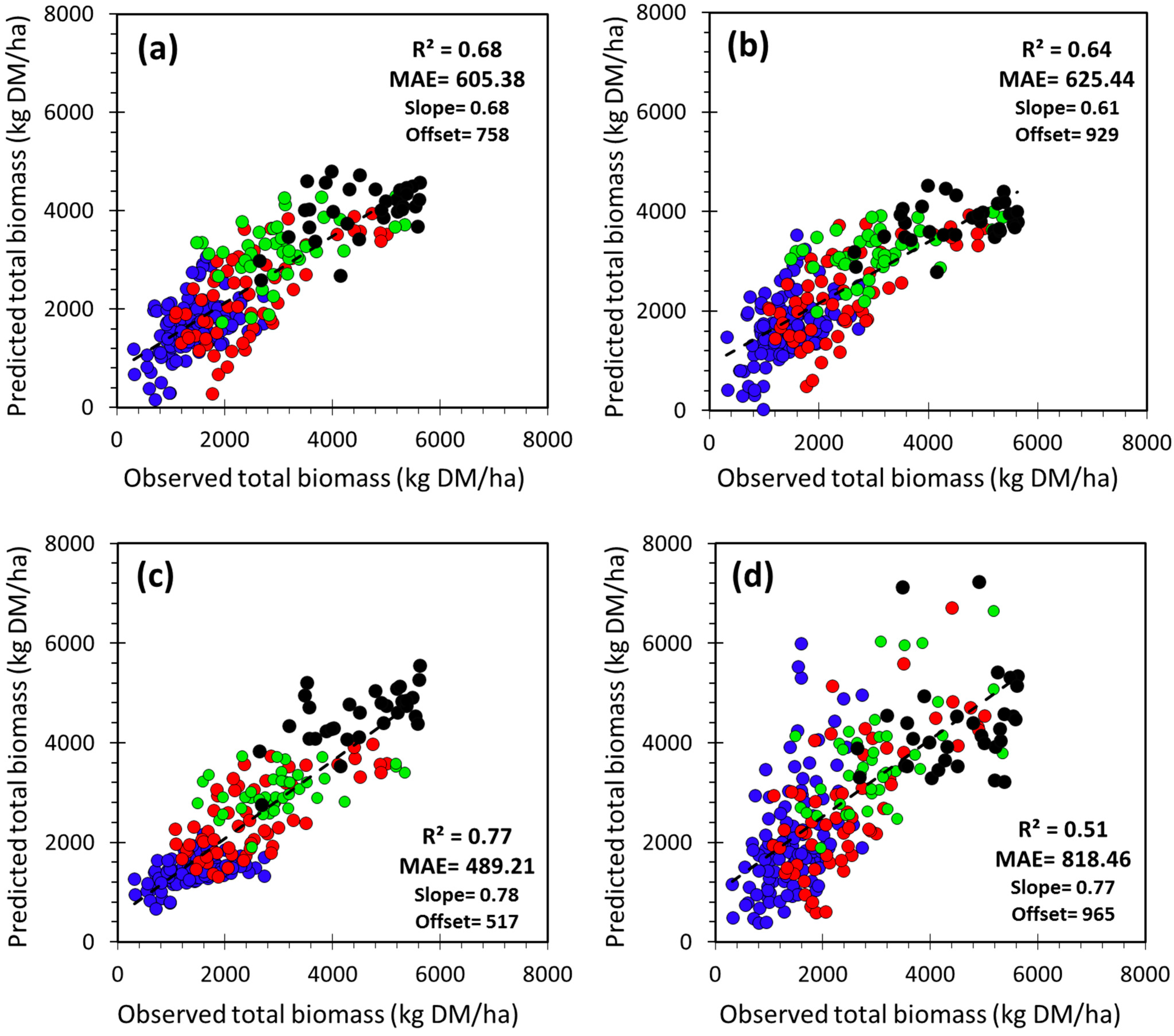
3.3. Selection and Verification of the Estimation Models
| Region | Estimation Model of Total Biomass (B) | Adj. R2 | MAE | NMAE | n/n_test | |
|---|---|---|---|---|---|---|
| (kg·DM/ha) | (%) | |||||
| Study area | Model_SA | B = 424.13 × LINTG − 100.91 × LOS + 39.80 × RDERIV + 293.71 | 0.67 | 608.13 | 26.0 | 263/39600 |
| Model_EW | B = 4594.18 × PEAK − 129.09 × SOS + 1866.17 | 0.62 | 641.04 | 27.3 | 263/39600 | |
| Ecoregion | ECOnorth | B = 1703.10 × PEAK + 1644.92 × BVAL + 432.94 | 0.24 | 426.85 | 31.0 | 121/18600 |
| ECOeast | B = 463.02 × LINTG − 296.29 × LOS − 152.37 × SOS + 5969.39 | 0.49 | 575.45 | 23.1 | 65/9800 | |
| ECOwest | B = 3341.72 × PEAK + 282.87 × PMID − 7125.91 | 0.15 | 589.29 | 19.1 | 44/6600 | |
| ECOsouth | B = 603.53 × LINTG + 52.83 × RDERIV − 325.30 × LOS + 1944.04 | 0.31 | 512.96 | 11.3 | 33/5000 | |
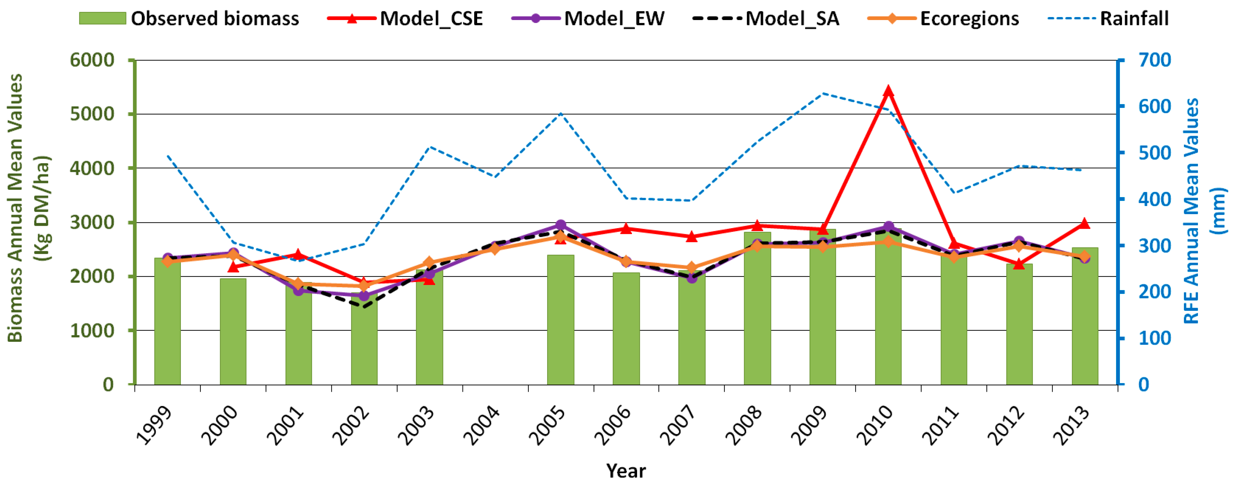
3.4. Comparison with the NDVI-Based CSE Biomass Product


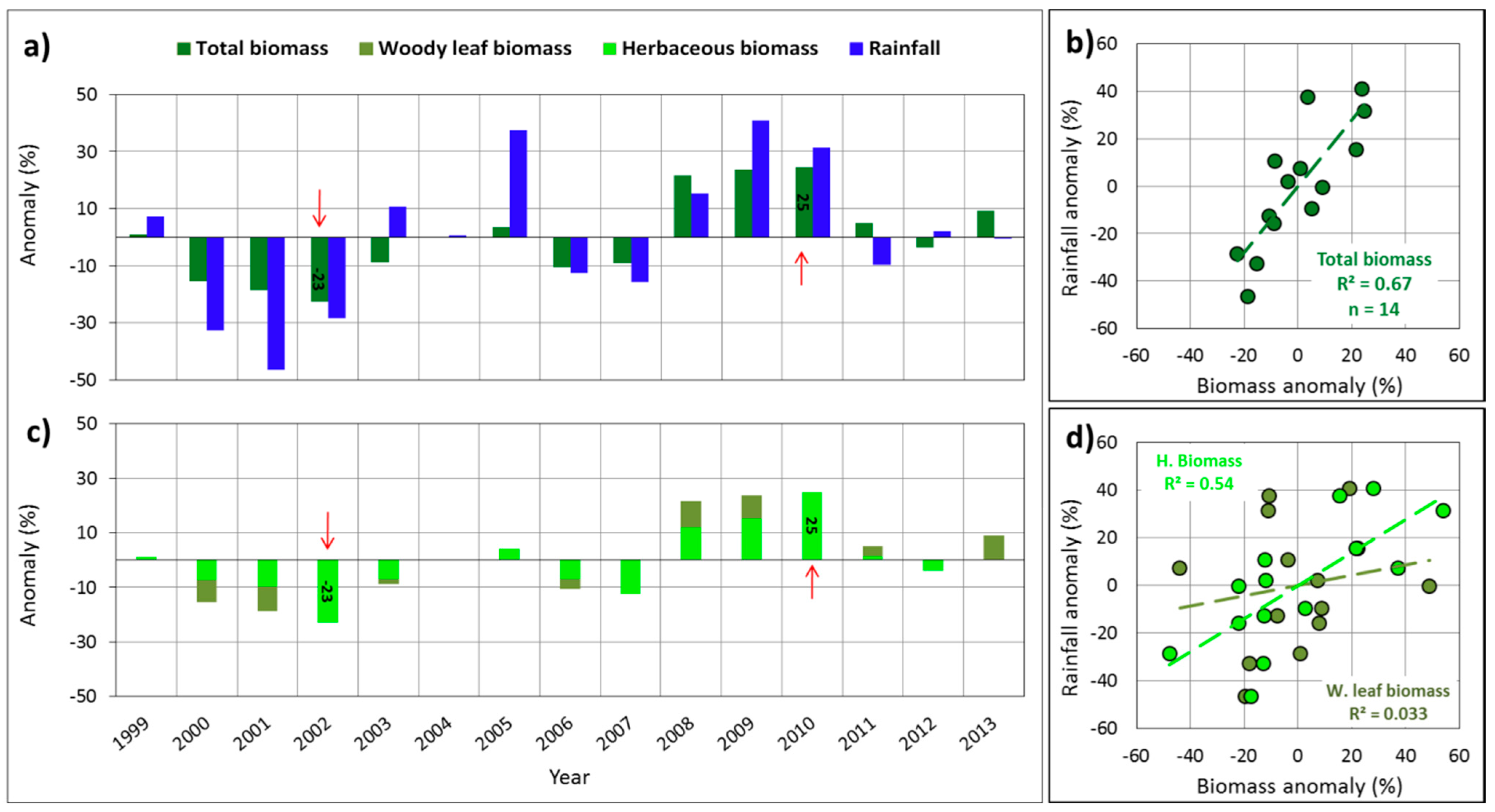
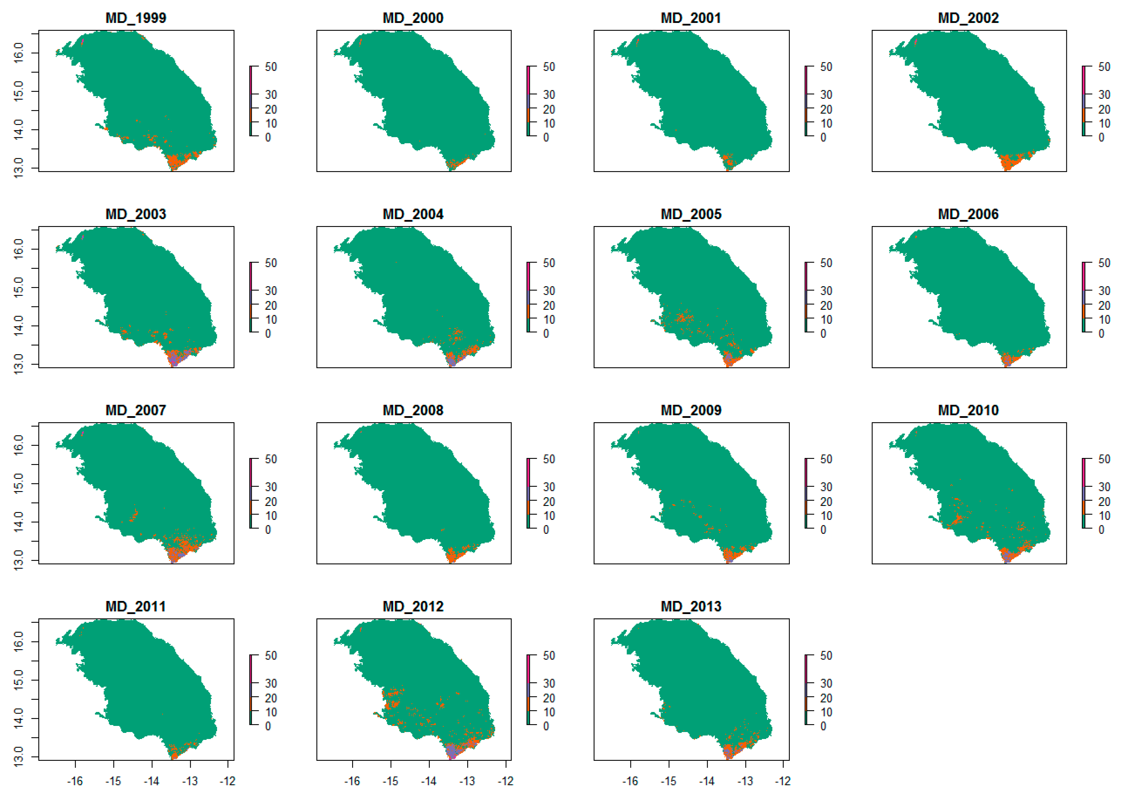
3.5. Testing the Multiple-Predictor Model for Early Warning
4. Discussion
5. Conclusions
Acknowledgments
Author Contributions
Conflicts of Interest
Appendix


References
- Alkemade, R.; Reid, R.S.; van den Berg, M.; de Leeuw, J.; Jeuken, M. Assessing the impacts of livestock production on biodiversity in rangeland ecosystems. Proc. Natl. Acad. Sci. USA 2012, 110. [Google Scholar] [CrossRef] [PubMed]
- Herrero, M.; Thornton, P.K. Livestock and global change: Emerging issues for sustainable food systems. Proc. Natl. Acad. Sci. USA 2013, 110, 20878–20881. [Google Scholar] [CrossRef] [PubMed]
- Dicko, M.S.; Djitèye, M.A.; Sangaré, M. Animal production systems in the sahel. Sécheresse 2006, 17, 83–97. [Google Scholar]
- Hickler, T.; Eklundh, L.; Seaquist, J.W.; Smith, B.; Ardö, J.; Olsson, L.; Sykes, M.T.; Sjöström, M. Precipitation controls sahel greening trend. Geophys. Res. Lett. 2005, 32, L21415. [Google Scholar] [CrossRef]
- Huber, S.; Fensholt, R. Analysis of teleconnections between AVHRR-based sea surface temperature and vegetation productivity in the semi-arid Sahel. Remote Sens. Environ. 2011, 115, 3276–3285. [Google Scholar] [CrossRef]
- Anyamba, A.; Small, J.; Tucker, C.; Pak, E. Thirty-two years of sahelian zone growing season non-stationary NDVI3g patterns and trends. Remote Sens. 2014, 6, 3101–3122. [Google Scholar] [CrossRef]
- Fensholt, R.; Sandholt, I.; Rasmussen, M.S. Evaluation of MODIS LAI, FAPAR and the relation between FAPAR and NDVI in a semi-arid environment using in situ measurements. Remote Sens. Environ. 2004, 91, 490–507. [Google Scholar] [CrossRef]
- Mbow, C.; Fensholt, R.; Nielsen, T.T.; Rasmussen, K. Advances in monitoring vegetation and land use dynamics in the Sahel. Geogr. Tidsskr. Dan. J. Geogr. 2014, 114, 84–91. [Google Scholar] [CrossRef]
- Atzberger, C. Advances in remote sensing of agriculture: Context description, existing operational monitoring systems and major information needs. Remote Sens. 2013, 5, 949–981. [Google Scholar] [CrossRef]
- Tucker, C.J.; Vanpraet, C.; Boerwinkel, E.; Gaston, A. Satellite remote sensing of total dry matter production in the Senegalese Sahel. Remote Sens. Environ. 1983, 13, 461–474. [Google Scholar] [CrossRef]
- Tucker, C.J.; Vanpraet, C.L.; Sharman, M.J.; Itterstum, G.V. Satellite remote sensing of total herbaceous biomass production in the Senegalese Sahel: 1980–1984. Remote Sens. Environ. 1985, 17, 233–249. [Google Scholar] [CrossRef]
- Diallo, O.; Diouf, A.; Hanan, N.P.; Ndiaye, A.; PrÉVost, Y. AVHRR monitoring of savanna primary production in Senegal, west Africa: 1987–1988. Int. J. Remote Sens. 1991, 12, 1259–1279. [Google Scholar] [CrossRef]
- Prince, S.D. Satellite remote sensing of primary production: Comparison of results for Sahelian grasslands 1981–1988. Int. J. Remote Sens. 1991, 12, 1301–1311. [Google Scholar] [CrossRef]
- Rasmussen, M.S. Assessment of millet yields and production in northern Burkina Faso using integrated NDVI from the AVHRR. Int. J. Remote Sens. 1992, 13, 3431–3442. [Google Scholar] [CrossRef]
- Mougenot, B.; Bégué, A.; Chehbouni, G.; Escadafal, R.; Heilman, P.; Qi, J.; Royer, A.; Watts, C. Applications of vegetation data to resource management in arid and semi-arid rangelands. In Proceedings of the VEGETATION-2000 Conference, Belgirate, Italy, 3–6 April 2000; pp. 433–434.
- Diouf, A.; Lambin, E.F. Monitoring land-cover changes in semi-arid regions: Remote sensing data and field observations in the Ferlo, Senegal. J. Arid Environ. 2001, 48, 129–148. [Google Scholar] [CrossRef]
- Bénié, G.B.; Kaboré, S.S.; Goïta, K.; Courel, M.F. Remote sensing-based spatio-temporal modeling to predict biomass in Sahelian grazing ecosystem. Ecol. Model. 2005, 184, 341–354. [Google Scholar] [CrossRef]
- Prince, S.D.; Goward, S.N. Global primary production: A remote sensing approach. J. Biogeogr. 1995, 22, 815–835. [Google Scholar] [CrossRef]
- Meroni, M.; Marinho, E.; Sghaier, N.; Verstrate, M.; Leo, O. Remote sensing based yield estimation in a stochastic framework—Case study of durum wheat in Tunisia. Remote Sens. 2013, 5, 539–557. [Google Scholar] [CrossRef] [Green Version]
- Baret, F.; Weiss, M.; Lacaze, R.; Camacho, F.; Makhmara, H.; Pacholcyzk, P.; Smets, B. Geov1: LAI and FAPAR essential climate variables and FCOVER global time series capitalizing over existing products. Part1: Principles of development and production. Remote Sens. Environ. 2013, 137, 299–309. [Google Scholar] [CrossRef]
- Fensholt, R.; Sandholt, I.; Rasmussen, M.S.; Stisen, S.; Diouf, A. Evaluation of satellite based primary production modelling in the semi-arid Sahel. Remote Sens. Environ. 2006, 105, 173–188. [Google Scholar] [CrossRef]
- Goward, S.N.; Huemmrich, K.F. Vegetation canopy PAR absorptance and the normalized difference vegetation index: An assessment using the SAIL model. Remote Sens. Environ. 1992, 39, 119–140. [Google Scholar] [CrossRef]
- Bégué, A. Leaf area index, daily intercepted PAR and spectral vegetation indices: A sensitivity analysis for regular-clumped canopies. Remote Sens. Environ. 1993, 46, 1–25. [Google Scholar] [CrossRef]
- Hanan, N.P.; Prince, S.D.; Bégué, A. Estimation of absorbed photosynthetically active radiation and vegetation net production efficiency using satellite data. Agric. Forest Meteorol. 1995, 76, 259–276. [Google Scholar] [CrossRef]
- Myneni, R.B.; Hall, F.B.; Sellers, P.J.; Marshak, A.L. The interpretation of spectral vegetation indices. IEEE Trans. Geosci. Remote Sens. 1995, 33, 481–486. [Google Scholar] [CrossRef]
- Le Roux, X.; Gauthier, H.; Bégué, A.; Sinoquet, H. Radiation absorption and use by humid savannah grassland, assessment using remote sensing and modelling. Agric. Forest Meteorol. 1997, 85, 117–132. [Google Scholar] [CrossRef]
- Lind, M.; Fensholt, R. The spatio-temporal relationship between rainfall and vegetation development in Burkina Faso. Geogr. Tidsskr. Dan. J. Geogr. 1999, 2, 43–55. [Google Scholar]
- Fensholt, R.; Sandholt, I.; Rasmussen, M.S.; Stisen, S. Improved primary production modelling in the semi-arid sahel using MODIS vegetation and stress indices combined with meteosat PAR data. Remote Sens. Environ. 2006, 105, 173–188. [Google Scholar] [CrossRef]
- Brandt, M.; Verger, A.; Diouf, A.A.; Baret, F.; Samimi, C. Local vegetation trends in the Sahel of Mali and Senegal using long time series FAPAR satellite products and field measurement (1982–2010). Remote Sens. 2014, 6, 2408–2434. [Google Scholar] [CrossRef]
- Neville, P.G. Controversy of variable importance in random forests. J. Unified Stat. Tech. 2013, 1, 15–20. [Google Scholar]
- Hanes, J.M.; Richardson, A.D.; Klostermann, S. Mesic temperate deciduous forest phenology. In Phenology: An Integrative Environmental Science, 2nd ed.; Schwartz, M.D., Ed.; Springer: New York, NY, USA, 2013; pp. 211–224. [Google Scholar]
- Colombo, R.; Busetto, L.; Fava, F.; Di Mauro, B.; Migliavacca, M.; Cremonese, E.; Galvagno, M.; Rossini, M.; Meroni, M.; Cogliati, S.; et al. Phenological monitoring of grassland and larch in the Alps from Terra and Aqua MODIS images. Ital. J. Remote Sens. 2011, 43, 83–96. [Google Scholar]
- Vrieling, A.; De Beurs, K.M.; Brown, M.E. Variability of african farming systems from phenological analysis of NDVI time series. Clim. Chang. 2011, 109, 455–477. [Google Scholar] [CrossRef]
- Meroni, M.; Rembold, F.; Verstraete, M.; Gommes, R.; Schucknecht, A.; Beye, G. Investigating the relationship between the inter-annual variability of satellite-derived vegetation phenology and a proxy of biomass production in the Sahel. Remote Sens. 2014, 6, 5868–5884. [Google Scholar] [CrossRef] [Green Version]
- Meroni, M.; Fasbender, D.; Kayitakire, F.; Pini, G.; Rembold, F.; Urbano, F.; Verstraete, M.M. Early detection of biomass production deficit hot-spots in semi-arid environment using FAPAR time series and a probabilistic approach. Remote Sens. Environ. 2014, 142, 57–68. [Google Scholar] [CrossRef]
- Brandt, M.; Mbow, C.; Diouf, A.A.; Verger, A.; Samimi, C.; Fensholt, R. Ground and satellite based evidence of the biophysical mechanisms behind the greening Sahel. Glob. Chang. Biol. 2015, 24, 1–11. [Google Scholar] [CrossRef] [PubMed]
- Funk, C.C.; Brown, M.E. Intra-seasonal NDVI change projections in semi-arid Africa. Remote Sens. Environ. 2006, 101, 249–256. [Google Scholar] [CrossRef]
- Herman, A.; Kumar, V.B.; Arkin, P.A.; Ko usky, J.V. Objectively determined 10-day African rainfall estimates created for famine early warning systems. Int. J. Remote Sens. 1997, 18, 2147–2159. [Google Scholar] [CrossRef]
- Tappan, G.G.; Sall, M.; Wood, E.C.; Cushing, M. Ecoregions and land cover trends in Senegal. J. Arid Environ. 2004, 59, 427–462. [Google Scholar] [CrossRef]
- Diouf, A.; Sall, M.; Wélé, A.; Dramé, M. Sampling Method of Primary Production in the Field; Technical Document; Centre de Suivi Ecologique of Dakar: Dakar, Senegal, 1998. [Google Scholar]
- Cissé, M.I. The browse production of some trees of the Sahel: Relationships between maximum foliage biomass and various physical parameters. In Browse in Africa; Houerou, H.N.L., Ed.; ILCA: Addis Ababa, Ethiopia, 1980; pp. 205–210. [Google Scholar]
- Hiernaux, P.H. Inventory of the browse potential of bushes, trees and shrubs in an area of the sahel in Mali: Method and initial results. In Browse in Africa; Houerou, H.N.L., Ed.; ILCA: Addis Ababa, Ethiopia, 1980; pp. 197–210. [Google Scholar]
- VITO—Flemish Institute for Technological Research. Template Product Information Package: S10 (spectral reflectance and NDVI). 2005. Available online: http://www.vgt4africa.org/PublicDocuments/S10-NDVI-Product-Sheet.pdf (accessed on 27 March 2015).
- Verger, A.; Baret, F.; Weiss, M. Performances of neural networks for deriving LAI estimates from existing cyclopes and MODIS products. Remote Sens. Environ. 2008, 112, 2789–2803. [Google Scholar] [CrossRef]
- Weiss, M.; Baret, F.; Garrigues, S.; Lacaze, R.; Bicheron, P. LAI, FAPAR and FCOVER cyclopes global products derived from vegetation. Part 2: Validation and comparison with MODIS collection 4 products. Remote Sens. Environ. 2007, 110, 317–331. [Google Scholar] [CrossRef]
- McCallum, I.; Wagner, W.; Schmullius, C.; Shvidenko, A.; Obersteiner, M.; Fritz, S.; Nilsson, S. Comparison of four global FAPAR datasets over northern Eurasia for the year 2000. Remote Sens. Environ. 2010, 114, 941–949. [Google Scholar] [CrossRef]
- Atkinson, P.M.; Jeganathan, C.; Dash, J.; Atzberger, C. Inter-comparison of four models for smoothing satellite sensor time-series data to estimate vegetation phenology. Remote Sens. Environ. 2012, 123, 400–417. [Google Scholar] [CrossRef]
- Fensholt, R.; Anyamba, A.; Stisen, S.; Sandholt, I.; Pak, E.; Small, J. Comparisons of compositing period length for vegetation index data from polar-orbiting and geostationary satellites for the cloud-prone region of west Africa. Photogramm. Eng. Remote Sens. 2007, 73, 297–309. [Google Scholar] [CrossRef]
- Chen, J.; Jönsson, P.; Tamura, M.; Gu, Z.; Matsushita, B.; Eklundh, L. A simple method for reconstructing a high-quality NDVI time-series data set based on the savitzky-Golay filter. Remote Sens. Environ. 2004, 91, 332–344. [Google Scholar] [CrossRef]
- Vintrou, E.; Bégué, A.; Baron, C.; Saad, A.; Lo Seen, D.; Traoré, S. A comparative study on satellite- and model-based crop phenology in west Africa. Remote Sens. 2014, 6, 1367–1389. [Google Scholar] [CrossRef] [Green Version]
- Jönsson, P.; Eklundh, L. Timesat—A program for analyzing time-series of satellite sensor data. Comput. Geosci. 2004, 30, 833–845. [Google Scholar] [CrossRef]
- Kandasamy, S.; Baret, F.; Verger, A.; Neveux, P.; Weiss, M. A comparison of methods for smoothing and gap filling time series of remote sensing observations: Application to MODIS LAI products. Biogeosciences 2013, 10, 4055–4071. [Google Scholar] [CrossRef]
- Verger, A.; Baret, F.; Weiss, M. A multisensor fusion approach to improve LAI time series. Remote Sens. Environ. 2011, 115, 2460–2470. [Google Scholar] [CrossRef]
- Verger, A.; Baret, F.; Weiss, M.; Kandasamy, S.; Vermote, E. The CACAO method for smoothing, gap filling and characterizing seasonal anomalies in satellite time series. IEEE Trans. Geosci. Remote Sens. 2013, 51, 1963–1972. [Google Scholar] [CrossRef]
- Eklundh, L.; Jönsson, P. Timesat 3.1 Manuel Software; Lund University: Lund, Sweden, 2011. [Google Scholar]
- Wold, S. Personal memories of the early PLS development. Chemom. Intell. Lab. Syst. 2001, 58, 83–84. [Google Scholar] [CrossRef]
- Afanador, N.L.; Tran, T.N.; Buydens, L.M.C. Use of the bootstrap and permutation methods for a more robust variable importance in the projection metric for partial least squares regression. Anal. Chim. Acta 2013, 768, 49–56. [Google Scholar] [CrossRef] [PubMed]
- Mehmood, T.; Liland, K.H.; Snipen, L.; Sæbø, S. A review of variable selection methods in partial least squares regression. Chemom. Intell. Lab. Syst. 2012, 118, 62–69. [Google Scholar] [CrossRef]
- Desbois, D. Introduction to partial least square regression with PLS procedure in SAS. Modulad 1999, 24, 41–97. [Google Scholar]
- Johnson, C.J.; Nielsen, S.E.; Merrill, E.H.; McDonald, T.E.; Boyce, M.S. Resource selection functions based on use-availability data: Theoretical motivation and evaluation methods. J. Wildl. Manag. 2006, 70, 347–357. [Google Scholar] [CrossRef]
- Kouadio, L.; Djaby, B.; Duveiller, G.; El Jarroudi, M.; Tychon, B. Decay kinetics of the green area and yield estimation of winter wheat. Biotechnol. Agron. Sociét. Environ. 2012, 5, 179–191. [Google Scholar]
- Confais, J.; Le Guen, M. First steps in linear regression with SAS. Modulad 2006, 35, 220–363. [Google Scholar]
- Belsley, D.A.; Kuh, E.; Welsh, R.E. Regression Diagnostics: Identifying Influential Data and Sources of Collinearity; Wiley: New York, NY, USA, 1980. [Google Scholar]
- Efron, B. The estimation of prediction error: Covariance penalties and cross-validation. J. Am. Stat. Assoc. 2004, 99, 619–632. [Google Scholar] [CrossRef]
- Borra, S.; Di Ciaccio, A. Measuring the prediction error. A comparison of cross-validation, bootstrap and covariance penalty methods. Comput. Stat. Data Anal. 2010, 54, 2976–2989. [Google Scholar] [CrossRef]
- Acquah, H.D.-G. A bootstrap approach to evaluating the performance of Akaike information criterion (AIC) and bayesian information criterion (BIC) in selection of an asymmetric price relationship. J. Agric. Sci. 2012, 57, 99–110. [Google Scholar] [CrossRef]
- Cole, S.R. Simple bootstrap statistical inference using the SAS system. Comput. Methods Programs Biomed. 1999, 60, 79–82. [Google Scholar] [CrossRef]
- Willmott, C.J.; Matsuura, K. Advantages of the mean absolute error (MAE) over the root mean square error (RMSE) in assessing average model performance. Clim. Res. 2005, 30, 79–82. [Google Scholar] [CrossRef]
- Dardel, C.; Kergoat, L.; Hiernaux, P.; Mougin, E.; Grippa, M.; Tucker, C.J. Re-greening Sahel: 30 years of remote sensing data and field observations (Mali, Niger). Remote Sens. Environ. 2014, 140, 350–364. [Google Scholar] [CrossRef]
- Richardson, A.D.; Black, T.A.; Ciais, P.; Delbart, N.; Friedl, M.A.; Gobron, N.; Hollinger, D.Y.; Kutsch, W.L.; Longdoz, B.; Luyssaert, S.; et al. Influence of spring and autumn phenological transitions on forest ecosystem productivity. Philos. Trans. R. Soc. B Biol. Sci. 2010, 365, 3227–3246. [Google Scholar] [CrossRef] [PubMed] [Green Version]
- Mbow, C.; Fensholt, R.; Rasmussen, K.; Diop, D. Can vegetation productivity be derived from greenness in a semi-arid environment? Evidence from ground-based measurements. J. Arid Environ. 2013, 97, 56–65. [Google Scholar] [CrossRef]
- Jin, Y.; Yang, X.; Qiu, J.; Li, J.; Gao, T.; Wu, Q.; Zhao, F.; Ma, H.; Yu, H.; Xu, B. Remote sensing-based biomass estimation and its spatio-temporal variations in temperate grassland, Northern China. Remote Sens. 2014, 6, 1496–1513. [Google Scholar] [CrossRef]
- Moron, V.; Robertson, A.W.; Ward, M.N. Seasonal predictability and spatial coherence of rainfall characteristics in the tropical setting of Senegal. Mon. Weather Rev. 2006, 134, 3248–3262. [Google Scholar] [CrossRef]
- Ivits, E.; Cherlet, M.; Horion, S.; Fensholt, R. Global biogeographical pattern of ecosystem functional types derived from earth observation data. Remote Sens. 2013, 5, 3305–3330. [Google Scholar] [CrossRef]
- Olsson, L.; Eklundh, L.; Ardö, J. A recent greening of the Sahel—Trends, patterns and potential causes. J. Arid Environ. 2005, 63, 556–566. [Google Scholar] [CrossRef]
- Diouf, A.A.; Djaby, B.; Diop, M.B.; Wele, A.; Ndione, J.A.; Tychon, B. Simple regression functions for estimating herbaceous fodder production in senegal rangelands from the s10 NDVI of SPOT-vegetation. In Proceedings of the 27th Symposium of the International Association of Climatology, Dijon, France, 2–5 July 2014; pp. 284–289.
- FAO—Food and Agriculture Organization of the United Nations. Executive Brief: The Sahel Crisis 2012. Available online: http://www.fao.org/fileadmin/user_upload/sahel/docs/EXECUTIVE%20BRIEF%20TCE%206%20July.pdf (accessed on 18 April 2015).
- DEPA—Direction de l’Elevage et des Productions Animales. Bilan Provisoire de l’Operation Sauvegarde du Bétail (OSB) 2012. Available online: http://csa.sn/site/index.php?option=com_phocadownload&view=category&download=86:amr-2012-contribution-elevage-osb-bilan-provisoirepdf&id=3:rapports-comptes-rendus&Itemid=61&start=12 (accessed on 28 March 2015).
- Verger, A.; Baret, F.; Weiss, M.; Filella, I.; Peñuelas, J. Geoclim: A global climatology of LAI, FAPAR, and FCOVER from vegetation observations for 1999–2010. Remote Sens. Environ. 2015. [Google Scholar] [CrossRef]
- Weiss, M.; Baret, F.; Lacaze, R.; Ramon, D.; Wandrebek, L.; Smets, B.; Verger, A. Near real time, global, LAI, FAPAR and cover fraction products derived from PROBA-V, at 300 m and 1 km resolution. In Proceedings of the Global Vegetation Monitoring and Modeling, Avignon, France, 3–7 February 2014.
- Lacaze, R.; Smets, B.; Calvet, J.C.; Camacho, F.; Tansey, K.; Baret, F.; Ramon, D.; Montersleet, B.; Roujean, J.L.; Wandrebek, L.; et al. Sentinel-3 for the copernicus global land service: Monitoring the continental ecosystems at global scale. In Proceedings of the Sentinel-3 for Science workshop, Venice, Italy, 2–5 June 2015.
- Mora, C.; Frazier, A.G.; Longman, R.J.; Dacks, R.S.; Walton, M.M.; Tong, E.J.; Sanchez, J.J.; Kaiser, L.R.; Stender, Y.O.; Anderson, J.M.; et al. The projected timing of climate departure from recent variability. Nature 2013, 502, 183–187. [Google Scholar] [CrossRef] [PubMed]
- Richardson, A.D.; Anderson, R.S.; Arain, M.A.; Barr, A.G.; Bohrer, G.; Chen, G.; Chen, J.M.; Ciais, P.; Davis, K.J.; Desai, A.R.; et al. Terrestrial biosphere models need better representation of vegetation phenology: Results from the north American carbon program site synthesis. Glob. Chang. Biol. 2012, 18, 566–584. [Google Scholar] [CrossRef]
© 2015 by the authors; licensee MDPI, Basel, Switzerland. This article is an open access article distributed under the terms and conditions of the Creative Commons Attribution license (http://creativecommons.org/licenses/by/4.0/).
Share and Cite
Diouf, A.A.; Brandt, M.; Verger, A.; Jarroudi, M.E.; Djaby, B.; Fensholt, R.; Ndione, J.A.; Tychon, B. Fodder Biomass Monitoring in Sahelian Rangelands Using Phenological Metrics from FAPAR Time Series. Remote Sens. 2015, 7, 9122-9148. https://doi.org/10.3390/rs70709122
Diouf AA, Brandt M, Verger A, Jarroudi ME, Djaby B, Fensholt R, Ndione JA, Tychon B. Fodder Biomass Monitoring in Sahelian Rangelands Using Phenological Metrics from FAPAR Time Series. Remote Sensing. 2015; 7(7):9122-9148. https://doi.org/10.3390/rs70709122
Chicago/Turabian StyleDiouf, Abdoul Aziz, Martin Brandt, Aleixandre Verger, Moussa El Jarroudi, Bakary Djaby, Rasmus Fensholt, Jacques André Ndione, and Bernard Tychon. 2015. "Fodder Biomass Monitoring in Sahelian Rangelands Using Phenological Metrics from FAPAR Time Series" Remote Sensing 7, no. 7: 9122-9148. https://doi.org/10.3390/rs70709122