Assessing Metrics for Estimating Fire Induced Change in the Forest Understorey Structure Using Terrestrial Laser Scanning

Abstract

Quantifying post-fire effects in a forested landscape is important to ascertain burn severity, ecosystem recovery and post-fire hazard assessments and mitigation planning. Reporting of such post-fire effects assumes significance in fire-prone countries such as USA, Australia, Spain, Greece and Portugal where prescribed burns are routinely carried out. This paper describes the use of Terrestrial Laser Scanning (TLS) to estimate and map change in the forest understorey following a prescribed burn. Eighteen descriptive metrics are derived from bi-temporal TLS which are used to analyse and visualise change in a control and fire-altered plot. Metrics derived are Above Ground Height-based (AGH) percentiles and heights, point count and mean intensity. Metrics such as AGH50_change, mean AGH_change and point count_change are sensitive enough to detect subtle fire-induced change (28%–52%) whilst observing little or no change in the control plot (0–4%). A qualitative examination with field measurements of the spatial distribution of burnt areas and percentage area burnt also show similar patterns. This study is novel in that it examines the behaviour of TLS metrics for estimating and mapping fire induced change in understorey structure in a single-scan mode with a minimal fixed reference system. Further, the TLS-derived metrics can be used to produce high resolution maps of change in the understorey landscape.

1. Introduction

Ecological systems are dynamic and disturbance is an important factor for change. Fire is an agent of environmental change globally at various spatial and temporal scales determining land use, productivity, biodiversity and has impacts on hydrologic, biogeochemical and atmospheric processes [1]. Fires occur over the majority of the Australian landscape and in most vegetation types [2], and Australian dry sclerophyll forests are amongst the more fire-prone forest communities in the world [3]. Land managers in such fire-prone countries mitigate the threat posed by catastrophic wildfires using prescribed burning (fuel reduction). These low intensity burns involve the deliberate application of fire to forest fuels under specified conditions in order to achieve well-defined management goals [4]. These goals include reduction of wildfire hazard, protecting biodiversity and protecting infrastructures at the urban interface [5].

Measuring the effects of a prescribed burn on the landscape (i.e., burn severity) is important for burn efficacy reporting [6] and allowing land managers to manage post-fire rehabilitation and remediation (e.g., to prevent runoff and erosion) [7,8]. Reporting following a prescribed burn can also help monitor ecosystem recovery [9] and quantify carbon emissions [10]. As such, land managers require an effective and meaningful way of quantifying burn severity.

Established techniques for describing or quantifying the effects of a fire include destructive sampling of the remaining fuel, in-situ visual estimates or measurement of post-burn variables [4]. Post-burn variables include percentage surface burnt, percentage understorey cover burnt (grass and litter), percentage canopy scorch and burnt and litter depth post-burn amongst others. Routinely used field measures of burn severity such as Composite Burn Index (CBI) are based on ocular estimation and judgement [11]. In Australia too, the techniques aimed at reporting the nature of the burn event using a number of variables to ascertain severity are also based on visual field assessments which are both subjective and qualitative [12]. The ability to draw accurate links between fire effects and operational fire models whilst overcoming cost, time and technical challenges posed to forest managers involved in collecting field data has also been acknowledged by several researchers [13,14,15]. In order to improve the reporting procedures around prescribed burns and quantify fire effects, a need for repeatable and quantified description has been identified in this paper.

Knowledge of the understorey environment is essential for fire behaviour modelling [15,16,17], wildlife habitat assessment and modeling [18] and carbon stocks and sequestration [19]. Hence, estimates of change in the understorey vegetation become important in burnt landscapes, however this has utility beyond fire severity mapping.

Airborne LiDAR technology has found wide utility in forest attribution [20,21,22,23,24,25,26]. Terrestrial Laser Scanning (TLS) is also increasingly being used to quantify forest properties such as canopy height [27], tree diameter [28,29,30], LAI [31,32] and canopy gap fraction [33]. These studies have focused on deriving a biophysical description of forests at a single point in time. Change detection in forested landscapes using LiDAR (both terrestrial and airborne) has been reported by many researchers [34,35,36,37]. However, this research has focused primarily on biomass accumulation or growth and dynamics of the canopy and emergent layers.

Detecting and quantifying the properties of the understorey using LiDAR technology has been less widely studied. Reported attempts [15,16] quantifying various properties of the understorey have utilised a variety of metrics derived from both airborne and terrestrial LiDAR data for fire-behaviour monitoring purposes as outlined in Table 1 ([14,15,17,18,38,39,40]). These metrics, which are primarily point density or height-based, have been used successfully to predict and estimate various understorey vegetation properties including volume, density, cover, height and biomass to varying degrees [17,38].

Table 1. LiDAR derived understorey metrics used by researchers to map understorey vegetation.

Metric	Property	Metric Type	Scale	LiDAR Platform	Application	Study
Proportion of corrected number of understorey laser hits	Cover	Point Density	Landscape	Airborne	Fire behaviour modelling	Riano et al. [15]
Proportion of corrected number of understorey laser hits	Cover	Point Density	Plot	Airborne	Ecological and forestry	Goodwin [38]
Presence or absence of laser points within each cm3 space	Volume	Point density	Plot	Terrestrial	Fire behaviour modelling	Loudermilk et al. [15]
% of ground returns % of returns between 1 and 2.5 m	Cover Distribution	Point Density	Plot	Airborne	Ecological management	Martinuzzi et al. [18]
Difference between pre- and post-fire LiDAR elevation	Cover Biomass	Height	Landscape	Airborne	Fire severity	Wang and Glen [39]
Variety of height metrics Ratio of Points Above and Below the Inflection Point	Cover	Both Point Density and Height	Plot	Terrestrial	Fire behaviour modelling	Rowel and Seielstad [17]
Proportion of number of understorey laser hits after applying intensity filter Number of LiDAR points per square metre under 1.5 m	Cover	Point Density	Plot	Airborne	Ecological management	Wing et al. [40]
Variety of Height-based Metrics	Cover Height	Height	Plot	Airborne	Wildfire behaviour modelling	Jakubowski et al. [14]

Table 1. LiDAR derived understorey metrics used by researchers to map understorey vegetation.

Metric	Property	Metric Type	Scale	LiDAR Platform	Application	Study
Proportion of corrected number of understorey laser hits	Cover	Point Density	Landscape	Airborne	Fire behaviour modelling	Riano et al. [15]
Proportion of corrected number of understorey laser hits	Cover	Point Density	Plot	Airborne	Ecological and forestry	Goodwin [38]
Presence or absence of laser points within each cm3 space	Volume	Point density	Plot	Terrestrial	Fire behaviour modelling	Loudermilk et al. [15]
% of ground returns % of returns between 1 and 2.5 m	Cover Distribution	Point Density	Plot	Airborne	Ecological management	Martinuzzi et al. [18]
Difference between pre- and post-fire LiDAR elevation	Cover Biomass	Height	Landscape	Airborne	Fire severity	Wang and Glen [39]
Variety of height metrics Ratio of Points Above and Below the Inflection Point	Cover	Both Point Density and Height	Plot	Terrestrial	Fire behaviour modelling	Rowel and Seielstad [17]
Proportion of number of understorey laser hits after applying intensity filter Number of LiDAR points per square metre under 1.5 m	Cover	Point Density	Plot	Airborne	Ecological management	Wing et al. [40]
Variety of Height-based Metrics	Cover Height	Height	Plot	Airborne	Wildfire behaviour modelling	Jakubowski et al. [14]

This paper is motivated by the successful use of point cloud based metrics to produce estimates of change in understorey properties. Given this success, LiDAR technology may provide an avenue to producing quantifiable and repeatable measurements of the effects of low intensity prescribed burns. This study explores the use of terrestrial LiDAR technology to produce estimates of understorey forest change which is accurate, repeatable, robust and sensitive to the low intensity nature of a prescribed burn and can be used by the land management agencies to supplement qualitative assessments of change in response to prescribed burns.

2. Method

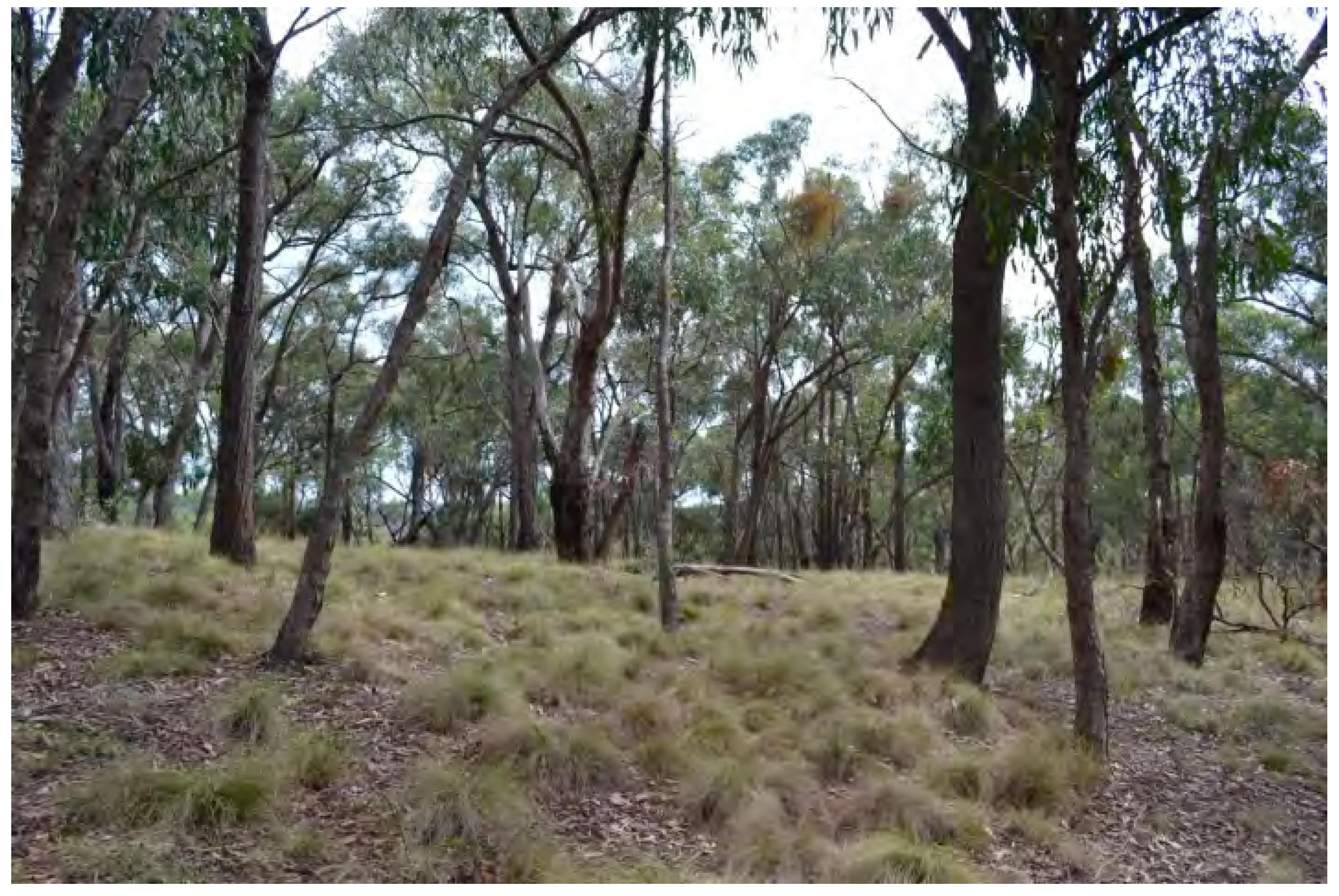
2.1. Study Area and Field Data

The study area was located in St Andrews, approximately 45 km northeast of metropolitan Melbourne, Victoria, Australia. The study was conducted in a dry sclerophyll forest with a grassy understorey (Figure 1). The site can be described as open Eucalypt woodland with an average canopy height between 10 and 12 m [41]. The midstorey vegetation layer was notably absent. The understorey was dominated by a variety of Tussock grass species with heights ranging from 30 to 50 cm. Two circular plots of 9 m radius were identified which were similar in topography (i.e., flat), vegetation species composition and arrangement. The extents of the plots were chosen to be close to the guidelines set out for the visual field assessment of burn severity developed by the Department of Environment, Land, Water and Planning (DELWP).

Figure 1. Dry sclerophyll forest with a grassy understorey in the study area.

Figure 1. Dry sclerophyll forest with a grassy understorey in the study area.

A planned burn was carried out by Parks Victoria and the DELWP on 15 April 2012. One plot received a fire treatment (fire-altered plot) which acted as the change agent while the other plot was left unburnt and acted as the control.

A burn severity assessment was conducted approximately two weeks after the planned burn on 27 April 2012. This visual assessment followed the methods described for use by local land managers [11]. The variables recorded in the understorey layer were percentage of the plot burnt, pre- and post-fire % cover (grass and litter), pre- and post-fire litter depth, post-fire leaf fall cover and char depth.

2.2. Terrestrial Laser Scanner and Surveys

The TLS instrument used in this research was a Trimble CX which utilises a combination of time-of-flight and phase-based measurement principles. The specifications are summarised in Table 2. Bi-temporal TLS data was acquired pre-burn on 8 March 2012 and post-burn on 30 April 2012 for each plot. All scans were obtained in a single-scan mode with the scanner located at the centre of the plot at an above ground height of 1.5 m. The angular point spacing was set to 1 cm at 10 m distance. The scans were performed to capture the scanner’s full range of view (360° horizontally and 300° vertically). Each hemispherical scan took approximately 45 min to complete. Co-registration between the bi-temporal scans was achieved by using permanent reference targets (stainless steel tags) fixed to stems within the plot.

Table 2. Specifications of the terrestrial LiDAR system (Trimble CX) used in this study.

Specification Type	Specification Value
Calibrated range	80 m to 90% reflective surface, 50 m to 18% reflective surface
Scan rate	54,000 points per second
Output angle accuracy	0.002° = 35 μrad (horizontal and vertical)
Vertical scanning angle	300°
Horizontal scanning angle	360°
Spot size	8 mm @ 25 m; 13 mm @ 50 m
Laser wavelength	660 nm (red)
Weight	11.8 kg
Dimensions (LxWxH)	12 × 52 × 35.5 cm
Power consumption	50 W

Table 2. Specifications of the terrestrial LiDAR system (Trimble CX) used in this study.

Specification Type	Specification Value
Calibrated range	80 m to 90% reflective surface, 50 m to 18% reflective surface
Scan rate	54,000 points per second
Output angle accuracy	0.002° = 35 μrad (horizontal and vertical)
Vertical scanning angle	300°
Horizontal scanning angle	360°
Spot size	8 mm @ 25 m; 13 mm @ 50 m
Laser wavelength	660 nm (red)
Weight	11.8 kg
Dimensions (LxWxH)	12 × 52 × 35.5 cm
Power consumption	50 W

2.3. Point Cloud Pre-Processing

The raw point clouds were processed following the steps depicted in Figure 2. Initially, the raw point clouds were exported to ASCII format using Trimble’s proprietary software (Trimble Realworks software version 6.5, 2009). Ground points were then identified in the fire-altered point clouds using the lasground tool of lastools [42]. We trialled several of the verbose options of lasground and visually assessed the results to determine the optimum combination for this landscape type. The “-not_airborne” option which is recommended for extracting ground points from terrestrial LiDAR data produced the best result and was therefore used to extract ground points. This allowed for a TIN representation of the ground surface to be generated. The final ground density after filtering was 2996.70 points/m². The Above Ground Height (AGH) of all points within the pre- and post-burn point clouds were then determined based on this ground surface representation. The ground points from the post-burn scans were used in the normalisation process of both pre- and post-burn point clouds to avoid introducing discrepancies in further analysis due to differing representations of the ground.

Points within the understorey were then selected as those with AGH between 5 and 100 cm. A minimum threshold was used due to uncertainty in ground detection results. This ensured any remaining ground points were excluded from the change detection analysis. The maximum threshold was selected based on the properties of the understorey vegetation in the study area. To avoid differences in occlusion between data capture events, caused by small variations in instrument set up for instance, points within areas deemed as occluded in one or both of the point clouds were removed from further analyses. This was achieved by creating a coverage map for each point cloud using the α-shape of the 2D point projections with α = 0.3 m. The coverage map was then used to clip the alternate point cloud.

This resulted in two sets of point clouds of pre and post-burn with equal areas of occlusion across the plot area. Understorey points were then assigned to 0.5 × 0.5 × 1.0 m voxels. Any voxels containing fewer than 10 points in either post- or pre-burn point clouds were considered still as being affected by occlusion. This approach also helped eliminate spurious points which were present in all point clouds. These corresponding voxels in both point clouds were removed from further analyses. The point count per voxel was >2000 in this research.

Figure 2. The work flow of the TLS data processing for deriving the understorey change detection metrics.

Figure 2. The work flow of the TLS data processing for deriving the understorey change detection metrics.

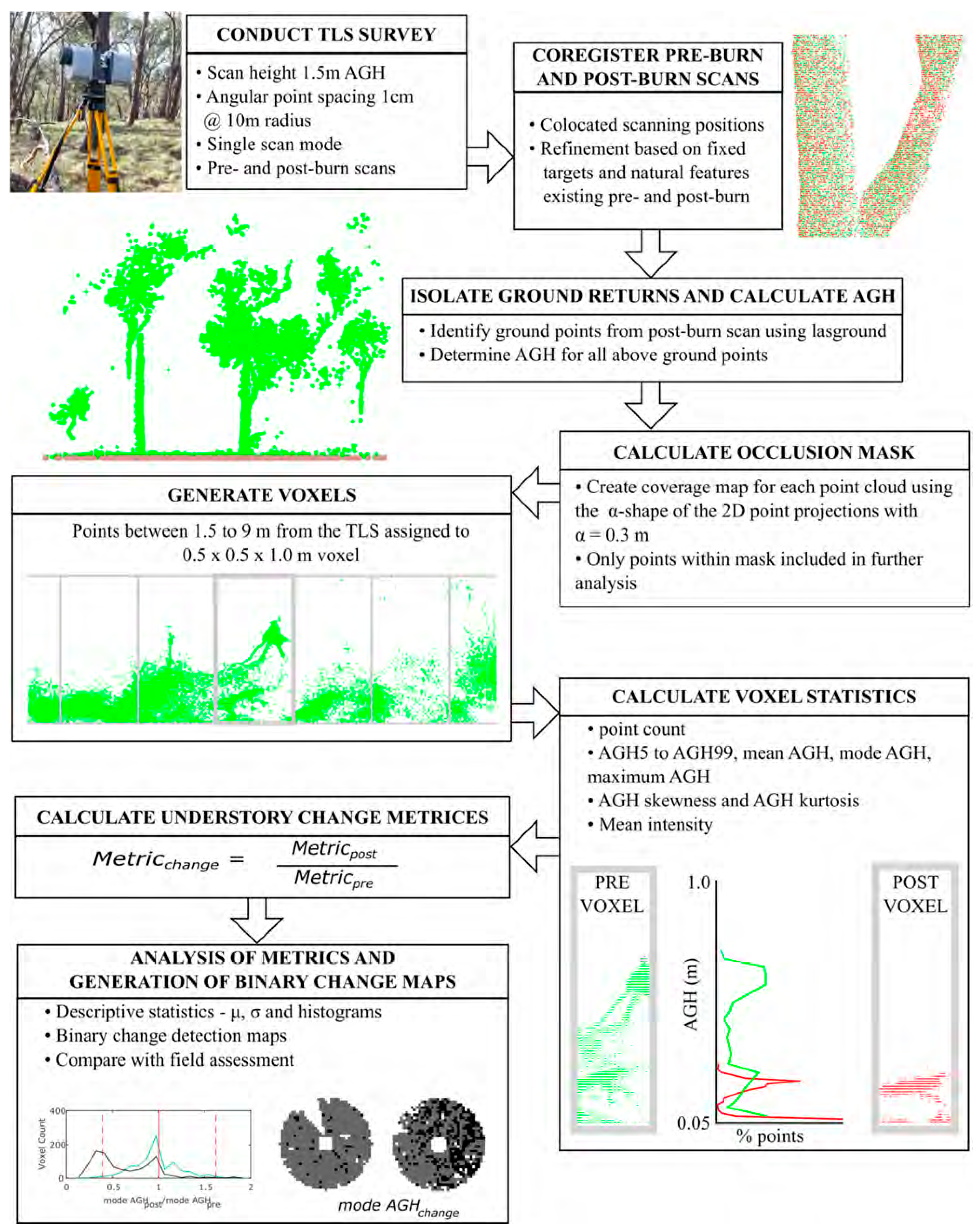
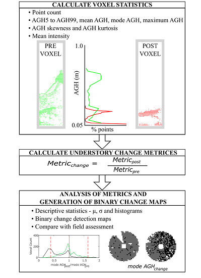
2.4. Metric Extraction

Change in the understorey is likely to be represented within each voxel’s point cloud as a change in the number of points or change in the AGH distribution. As such, for each point cloud metrics describing these properties were derived for each voxel. These are listed in Table 3. In all, a total of 18 metrics were extracted and tested.

Table 3. TLS-derived metrics used in this research to characterise change in forest understorey. These metrics were computed for each voxel in both pre- and post-burn point clouds.

Metric Name	Metric Description
AGH10, AGH20…AGH90, AGH95	Above Ground Height Percentiles (AGH50 is median height)
AGH mean	Mean Above Ground Height
AGH mode	Mode Above Ground Height
AGH maximum	Maximum Above Ground Height
AGH skewness	Skewness of Above Ground Height
AGH kurtosis	Kurtosis of Above Ground Height
Mean intensity	Mean intensity of TLS returns
Point count	Point count of TLS returns

Table 3. TLS-derived metrics used in this research to characterise change in forest understorey. These metrics were computed for each voxel in both pre- and post-burn point clouds.

Metric Name	Metric Description
AGH10, AGH20…AGH90, AGH95	Above Ground Height Percentiles (AGH50 is median height)
AGH mean	Mean Above Ground Height
AGH mode	Mode Above Ground Height
AGH maximum	Maximum Above Ground Height
AGH skewness	Skewness of Above Ground Height
AGH kurtosis	Kurtosis of Above Ground Height
Mean intensity	Mean intensity of TLS returns
Point count	Point count of TLS returns

In order to map and comparatively assess the likelihood of change indicated by each of these metrics, the proportion of post- and pre-burn measures was computed following Equation (1). The use of proportion to assess change approach allowed for a unitless comparison between metrics and also accounts for variations in some of the laser properties which are affected by the radial distance from the scanner (i.e., point count decreases towards the edge of the plot).

Metric_change = Metric_post-burn/Metric_pre-burn

(1)

A value for Metric_change close to 1 indicates that no change has occurred in the metric between scans. Voxels with Metric_change value of less than 1 indicate a decrease in that metric and a value of greater than 1 indicates that the metric has increased. It is expected that a loss of understorey biomass due to burn will create a decrease in most metrics including the point count and AGH percentiles. For each change metric, Mean (μ) and Standard Deviation (σ) for the population of voxels in each plot pre and post-burn was computed. A voxel was determined to have been altered by the burn where the change detected by the metric was greater than μ_control ± 1.64 × σ_control (90% confidence interval). This allowed a burn map to be generated. Finally, in order to provide a quantified estimated of change the understory height differences were computed based on differences in AGH95 and AGH99.

The μ_control and σ_control are being used because the control plot represents the “natural-change” environment. In a no-change environment, the ratio-based metrics should show a value of 1 between the post- and pre-burn measures in the control plot indicative of no change. Nonetheless, some change is expected to occur in the control plot. These are expected to be subtle and may include phenological change, wildlife movement and wildlife foraging activity. This approach also allows any small errors in co-registration of the point clouds to be excluded from being mapped as change.

2.5. Occlusion Impact Assessment

TLS surveys were performed in single-scan mode to allow for the most rapid data collection. Nevertheless, occlusion has been identified as a major issue for measuring forest properties with TLS technology [43]. In order to assess the impact of occlusion on the ability of the metrics to remain robust and detect change in the vegetated understorey bootstrapping analysis was applied. Stems (modelled as cylinders of random diameter between 0.1 and 0.5 m) were created and placed in the plot. All points which would have been occluded by the stem were them removed. Modelled stems were randomly located within the plot to simulate visible plot areas at 5% increments from 5% to 70%. Figure 3 shows some randomly generated stem maps. Bootstrapping analysis was then applied on the voxels of the two plots with n = 50. The μ and σ was then calculated for all the TLS-derived metrics.

Figure 3. Randomly generated stem maps simulating plot coverage at 10%, 30%, 50% and 70%, respectively. Red areas correspond to visible plot area.

Figure 3. Randomly generated stem maps simulating plot coverage at 10%, 30%, 50% and 70%, respectively. Red areas correspond to visible plot area.

2.6. Metric Assessment

The criteria for metric’s ability to detect change induced by prescribed burn were based on three factors: sensitivity, stability and similarity. Sensitivity relates to the ability of the metric to detect change (in the fire-altered plot). Stability relates to the metric showing the least change in the control plot which was assessed based on the µ, σ of Metric_change in the control plot along with % voxels recording change. Similarity relates to the ability of the metric to identify spatial patterns of change which are similar to visual assessments. To summarise, to be used in measuring fire effects in the understorey, TLS derived metrics should detect very little change in the control plot whilst detecting a change in the fire-altered plot that matches well with true change on the ground.

3. Results

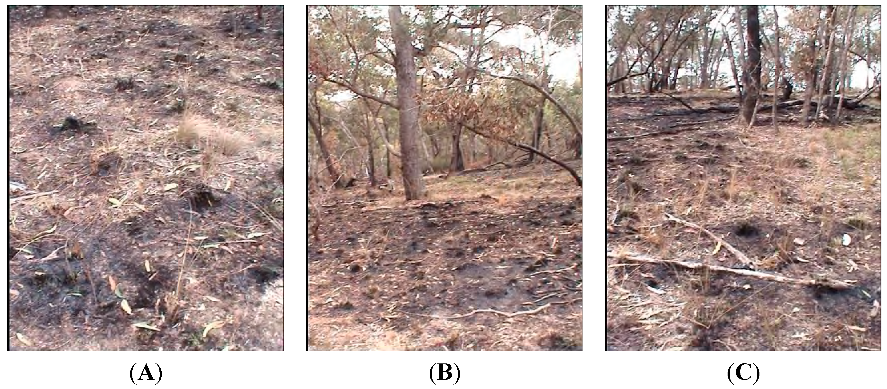
3.1. Field Assessment

As expected, the control plot which received no fire treatment showed no discernible change due to the burn. However, defoliation of a fallen tree in the south east region of the plot represented a loss of biomass within the height range of the voxels between surveys resulting in a small, localised change. The qualitative field assessment suggested that the prescribed burn resulted in a mosaic burn pattern with 60%–70% of the plot estimated to be affected by fire. Figure 4A demonstrates the patchy nature of prescribed burn. The understorey forest on the eastern side of the plot showed a larger and uniform burnt area as compared to the west (Figure 4B) and. a large unburnt area in the south-western edge of the plot slightly away from the plot centre (Figure 4C). Apart from that, there were unburnt patches interspersed with burnt patches all around the plot. The severity class identified based on the field assessments suggested a variable intensity of fire ranging from a warm ground burn to an intense understorey fire.

Figure 4. (A) Patchiness of low intensity prescribed burns that result in a mosaic landscape of burnt and unburnt patches; (B) A large burnt area on the eastern side of the fire-altered plot; (C) Part of the unburnt patch in the south-western side of the fire-altered plot.

Figure 4. (A) Patchiness of low intensity prescribed burns that result in a mosaic landscape of burnt and unburnt patches; (B) A large burnt area on the eastern side of the fire-altered plot; (C) Part of the unburnt patch in the south-western side of the fire-altered plot.

3.2. TLS Change Detection

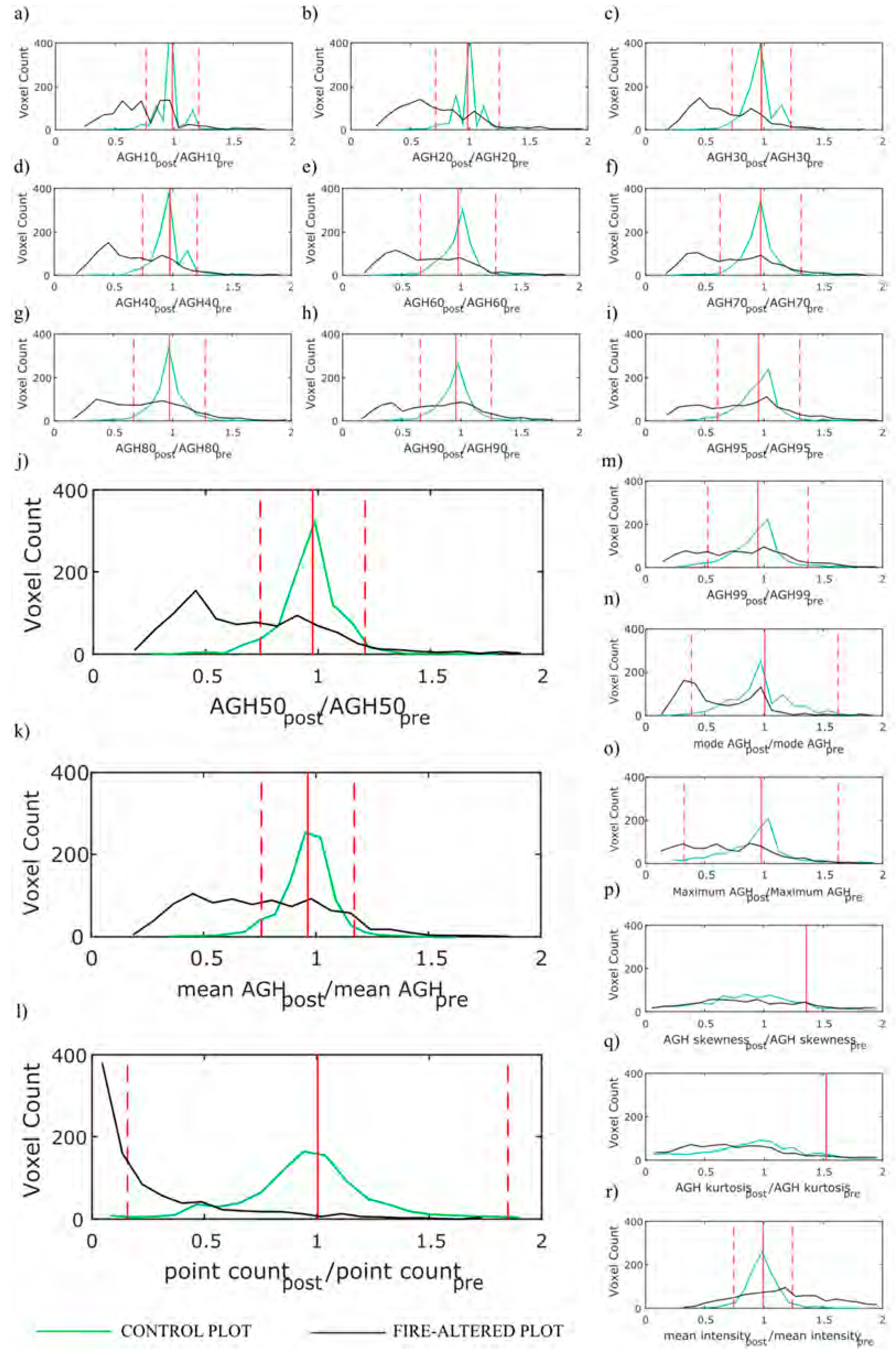
3.2.1. Descriptive Statistics

In 16 of the 18 TLS-derived metrics, the mean of the change metrics in the control plot varied between 0.95 and 1.01 (σ = 0.14 − 0.45) as listed in Table 4. The mean for both AGH skewness_change and AGH kurtosis_change were exceptions to this trend and showed a much higher value of 1.36 (σ = 10.91) and 1.53 (σ = 2.84), respectively. Percentage of voxels in the control plot which were classified as having undergone change varied between 1% and 9% for all 18 metrics.

In the fire-altered plot, the metrics showed a much more diverse mean change which was recorded in the range of 0.48–1.19 (σ = 0.32 − 1.67) in contrast to the control plot. The percentage change recorded by these metrics was in the range of 18%–52%. The percentage of voxels affected by change because of the fire varied between 22% and 71%. AGH skewness_change showed a mean value of 1.39 (σ = 17.06) which was quite similar to that from the control (µ = 1.36, σ = 10.91). AGH skewness_change showed a lower mean value of 1.29 (σ = 2.09) in the fire-altered plot as compared to the control (µ = 1.53, σ = 2.84). The percentage of voxels identified as having undergone a change in the fire-altered plot was 3% and 2% for AGH skewness_change and AGH kurtosis_change, respectively.

The change in understorey vegetation height as computed by AGH95 and AGH99 metrics in the two plots is listed in Table 5. The mean change in the control plot was 2 cm and 3 cm (σ = 7 − 11 cm) for the AGH95 and AGH99 metrics, respectively, as compared to 6 cm and 9 cm (σ = 16 − 20 cm) in the fire-altered plot. This is a very small change at the plot level.

Table 4. Descriptive statistics of the change detected by the various TLS-derived metrics and number of change voxels examined for the control and fire-altered plot. Statistics presented are aggregates of all voxels in each plot. Voxels recording a change have been computed as those having values greater than ± 1.64 × σ of µ for that particular metric.

Metric	Control Plot				Fire-Altered Plot
	Statistic		Change		Statistic		Change
	Mean (µ)	Standard Deviation (σ)	Number of Voxels	% of Voxels (n = 872)	Mean (µ)	Standard Deviation (σ)	Number of Voxels	% of Voxels (n = 925)
AGH10change	0.99	0.14	60	7	0.76	0.38	587	63
AGH20change	0.98	0.16	41	5	0.72	0.37	571	62
AGH30change	0.98	0.15	57	7	0.72	0.38	604	65
AGH40change	0.98	0.14	78	9	0.71	0.37	623	67
AGH50change	0.98	0.14	64	7	0.72	0.36	598	65
AGH60change	0.97	0.19	32	4	0.74	0.37	491	53
AGH70change	0.97	0.21	31	4	0.76	0.38	449	49
AGH80change	0.96	0.18	44	5	0.79	0.39	475	51
AGH90change	0.95	0.18	56	6	0.82	0.42	451	49
AGH95change	0.95	0.21	54	6	0.85	0.44	400	43
AGH99change	0.95	0.26	69	8	0.82	0.44	344	37
mean AGHchange	0.96	0.13	70	8	0.76	0.32	563	61
mode AGHchange	1.01	0.38	39	4	0.70	0.54	320	35
maximum AGHchange	0.98	0.40	70	8	0.70	0.38	199	22
AGH skewnesschange	1.36	10.91	6	1	1.39	17.06	26	3
AGH kurtosischange	1.53	2.84	29	3	1.29	2.09	19	2
point countchange	1.00	0.45	37	4	0.48	1.67	653	71
mean intensitychange	0.99	0.15	64	7	1.19	0.41	506	55

Table 4. Descriptive statistics of the change detected by the various TLS-derived metrics and number of change voxels examined for the control and fire-altered plot. Statistics presented are aggregates of all voxels in each plot. Voxels recording a change have been computed as those having values greater than ± 1.64 × σ of µ for that particular metric.

Metric	Control Plot				Fire-Altered Plot
	Statistic		Change		Statistic		Change
	Mean (µ)	Standard Deviation (σ)	Number of Voxels	% of Voxels (n = 872)	Mean (µ)	Standard Deviation (σ)	Number of Voxels	% of Voxels (n = 925)
AGH10change	0.99	0.14	60	7	0.76	0.38	587	63
AGH20change	0.98	0.16	41	5	0.72	0.37	571	62
AGH30change	0.98	0.15	57	7	0.72	0.38	604	65
AGH40change	0.98	0.14	78	9	0.71	0.37	623	67
AGH50change	0.98	0.14	64	7	0.72	0.36	598	65
AGH60change	0.97	0.19	32	4	0.74	0.37	491	53
AGH70change	0.97	0.21	31	4	0.76	0.38	449	49
AGH80change	0.96	0.18	44	5	0.79	0.39	475	51
AGH90change	0.95	0.18	56	6	0.82	0.42	451	49
AGH95change	0.95	0.21	54	6	0.85	0.44	400	43
AGH99change	0.95	0.26	69	8	0.82	0.44	344	37
mean AGHchange	0.96	0.13	70	8	0.76	0.32	563	61
mode AGHchange	1.01	0.38	39	4	0.70	0.54	320	35
maximum AGHchange	0.98	0.40	70	8	0.70	0.38	199	22
AGH skewnesschange	1.36	10.91	6	1	1.39	17.06	26	3
AGH kurtosischange	1.53	2.84	29	3	1.29	2.09	19	2
point countchange	1.00	0.45	37	4	0.48	1.67	653	71
mean intensitychange	0.99	0.15	64	7	1.19	0.41	506	55

Table 5. Summary statistics of the absolute change in height detected by AGH95 and AGH99. Statistics presented are aggregates of all voxels in each plot.

Metric	Control Plot		Fire-Altered Plot
	Mean (µ)	Standard Deviation (σ)	Mean (µ)	Standard Deviation (σ)
AGH95	2 cm	7 cm	6 cm	16 cm
AGH99	3 cm	11 cm	9 cm	20 cm

Table 5. Summary statistics of the absolute change in height detected by AGH95 and AGH99. Statistics presented are aggregates of all voxels in each plot.

Metric	Control Plot		Fire-Altered Plot
	Mean (µ)	Standard Deviation (σ)	Mean (µ)	Standard Deviation (σ)
AGH95	2 cm	7 cm	6 cm	16 cm
AGH99	3 cm	11 cm	9 cm	20 cm

Histogram distributions between the control and fire-altered plot for all the TLS metrics were plotted to ascertain if fire induced change was discernible. It is evident from Figure 5 that there were clear differences between the two plots across all but two metrics (AGH skewness_change and AGH kurtosis_change). General trends suggest that histogram distributions were approximately normal in the control plot for most metrics. In the fire-altered plot most of the metrics exhibited either multi- or bi-modal distributions.

Figure 5. Histograms of voxels for the TLS-derived metrics (a) AGH10_change, (b) AGH20_change, (c) AGH30_change, (d) AGH40_change, (e) AGH60_change, (f) AGH70_change, (g) AGH80_change, (h) AGH90_change, (i) AGH95_change, (j) AGH50_change, (k) mean AGH_change, (l) point count _change, (m) AGH99_change, (n) mode AGH_change, (o) maximum AGH_change, (p) AGH skewness_change, (q) AGH kurtosis_change, and (r) mean intensity_change in the control and fire-altered plot. The solid red line indicates µ change for that metric in the control plot. Voxels with values outside of the range defined by the dashed red lines (µ ± 1.64 × σ) are considered as fire-altered.

Figure 5. Histograms of voxels for the TLS-derived metrics (a) AGH10_change, (b) AGH20_change, (c) AGH30_change, (d) AGH40_change, (e) AGH60_change, (f) AGH70_change, (g) AGH80_change, (h) AGH90_change, (i) AGH95_change, (j) AGH50_change, (k) mean AGH_change, (l) point count _change, (m) AGH99_change, (n) mode AGH_change, (o) maximum AGH_change, (p) AGH skewness_change, (q) AGH kurtosis_change, and (r) mean intensity_change in the control and fire-altered plot. The solid red line indicates µ change for that metric in the control plot. Voxels with values outside of the range defined by the dashed red lines (µ ± 1.64 × σ) are considered as fire-altered.

Histogram distribution of voxels in the control plot was approximately normal when computed using metrics such as AGH50_change to AGH99_change, mean AGH_change, point count_change and mean intensity_change. For these metrics the mode was centred between 0.9 and 1.0 with the mean and mode being coincidental. The histogram distribution of point count_change metric (Figure 5l) was slightly flatter in comparison to the metrics which were normally distributed (AGH50_change to AGH99_change, mean AGH_change, and mean intensity_change). This is demonstrated by the large σ value recorded by point count_change at 0.45 in comparison to the abovementioned metrics (σ = 0.14 − 0.26).

Histogram distributions for other metrics such as AGH10_change to AGH40_change, (Figure 5a–d) and mode AGH_change (Figure 5n) showed multiple peaks in the control plot. The common factor between the histograms of these metrics is that the mode was centred between 0.9 and 1.0. The peaks in the histograms for these metrics was seen to occur at 1.1–1.2. AGH metrics such as AGH10_change and AGH20_change exhibited a minor peak centred at 0.7–0.8 (Figure 5a,b). Histogram distribution of AGH95_change, AGH99_change and maximum AGH_change (Figure 5i,m,o) exhibited a slight negative skew with the mode centred at 1.0–1.1. AGH skewness_change and AGH kurtosis_change (Figure 5p,q) histogram distribution was very flattish in comparison to the distribution of other metrics from the control plot. Both these metrics showed a very large variance.

The histogram distributions of the TLS-derived metrics were very different in the fire-altered plot. None of the distributions except point count_change (Figure 5l) were unimodal. Histogram distribution of point count_change was extremely positively skewed with the mode centred between 0 and 0.10. AGH10_change (Figure 5a) distribution was multimodal with peaks at 0.4–0.5, 0.6–0.7, 0.8–0.9 and 0.9–1.0. Distributions of AGH20_change to AGH95_change and mode AGH_change were nearly bimodal with 0.4–0.5 and 0.8–0.9. For the remaining metrics (AGH99_change, mean AGH_change, maximum AGH_change, AGH skewness_change, AGH kurtosis_change, AGH intensity_change), the distribution was comparatively flat. The distribution of both AGH skewness_change and AGH kurtosis_change from the fire-altered plot in particular were similar to those from the control plot (Figure 5p,q). Histogram distribution of mean intensity_change (Figure 5r) was flatter in the fire-altered plot with a large variance. Barring the histogram distribution of AGH skewness_change and AGH kurtosis_change all others exhibited a much higher variation in the fire-altered plot in contrast to the control plot whilst also showing a change in the distribution.

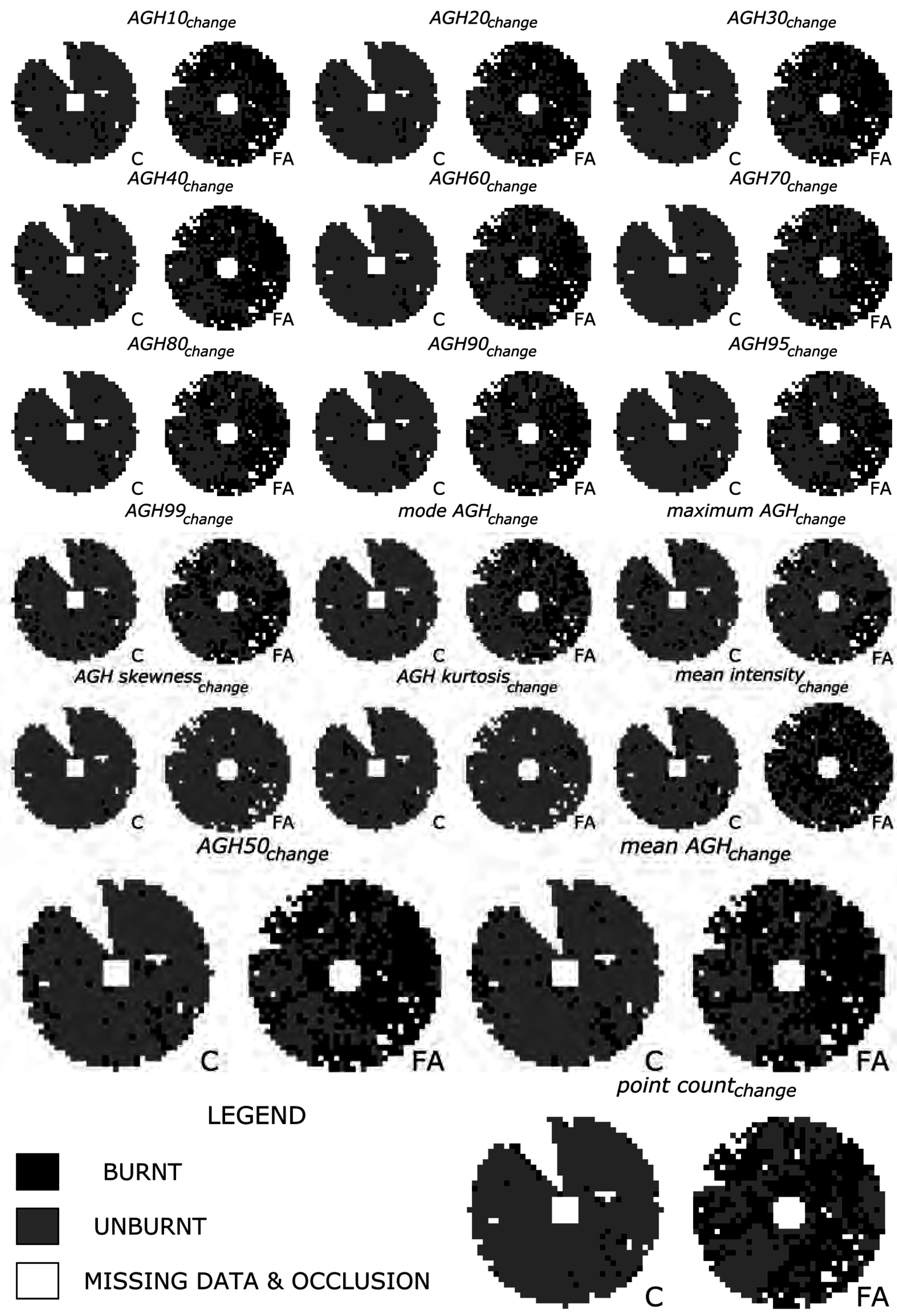
3.2.2. Spatial Distribution of Change

The spatial distribution of change detected by the 18 TLS derived metrics in the two plots is presented in Figure 6 as binary maps of “change” and “no change” categories. This figure shows that no metrics reported a change (greater than µ ± 1.64 × σ) in the majority of the control plot. The percentage of plot area that showed a change in the control plot corresponded to 1%–9% of the voxels. In contrast, in the fire altered plot change was detected in 22%–71% of the voxels using 16 of the 18 TLS-derived metrics (except AGH skewness_change and AGH kurtosis_change). AGH skewness_change and AGH kurtosis_change showed no difference between the control and fire-altered plot.

The spatial pattern and distribution of change in the control plot did not vary as much between the various metrics. There was some systematic change observed towards the south eastern part of the control plot using the AGH_change percentiles (except AGH99_change), mean AGH_change, point count_change and mean intensity_change.

This region of change found in the control plot was at the location of the defoliated fallen tree. Apart from this the little change detected by all the metrics in the control plot appeared to be random with little evidence of clustering as is evident from Figure 6.

Figure 6. Spatial distribution of change detected by the various TLS-derived metrics in the control (C) and fire-altered (FA) plot. Blank areas correspond to occluded voxels or missing data. Areas of no change (grey) were calculated as having values within ± 1.64 × σ of the µ from the control plot.

Figure 6. Spatial distribution of change detected by the various TLS-derived metrics in the control (C) and fire-altered (FA) plot. Blank areas correspond to occluded voxels or missing data. Areas of no change (grey) were calculated as having values within ± 1.64 × σ of the µ from the control plot.

In the fire-altered plot, the spatial pattern of change was markedly different as compared to the control plot. % of voxels affected by the fire ranged between 62% and 67% for AGH10_change to AGH50_change metrics. Most of the change detected by these five metrics was in the eastern and northern part of the plot with small unburnt patches interspersed. Most of the unburnt area was around the west and south western edge of the plot. The change detected by the remaining AGH_change percentiles decreased from 53% (AGH60_change) to 37% (AGH99_change).

These upper AGH_change percentiles detected more unburnt areas in north and northwest edge of the plot. AGH95_change and AGH99_change in particular detected patchy burnt areas within large contiguous unburnt areas which were quite opposite to the pattern of change detected by other AGH_change percentiles and field assessments of plot areas burnt. These two metrics also detected a large burnt area only in a small section of the south-eastern edge of the plot. Spatial pattern of change detected by maximum AGH_change and mode AGH_change was similar to AGH99_change. Maximum AGH_change detected even lesser burnt patches (22%) as compared to mode AGH_change (35%). Mean AGH_change detected change similar to AGH10_change to AGH50_change (61%). Point count_change metric detected change in 71% of the voxels of the fire-altered plot. Patches of no change were limited to the southwest part of the plot and smaller patches elsewhere interspersed with large patches of burnt areas especially in the western side. The pattern of change detected by Point count_change was somewhat comparable to AGH10_change to AGH50_change and mean AGH_change. The mean intensity_change metric showed an extremely patchy pattern with random burnt and unburnt areas throughout the fire-treated plot distinct from the change detected by the other metrics.

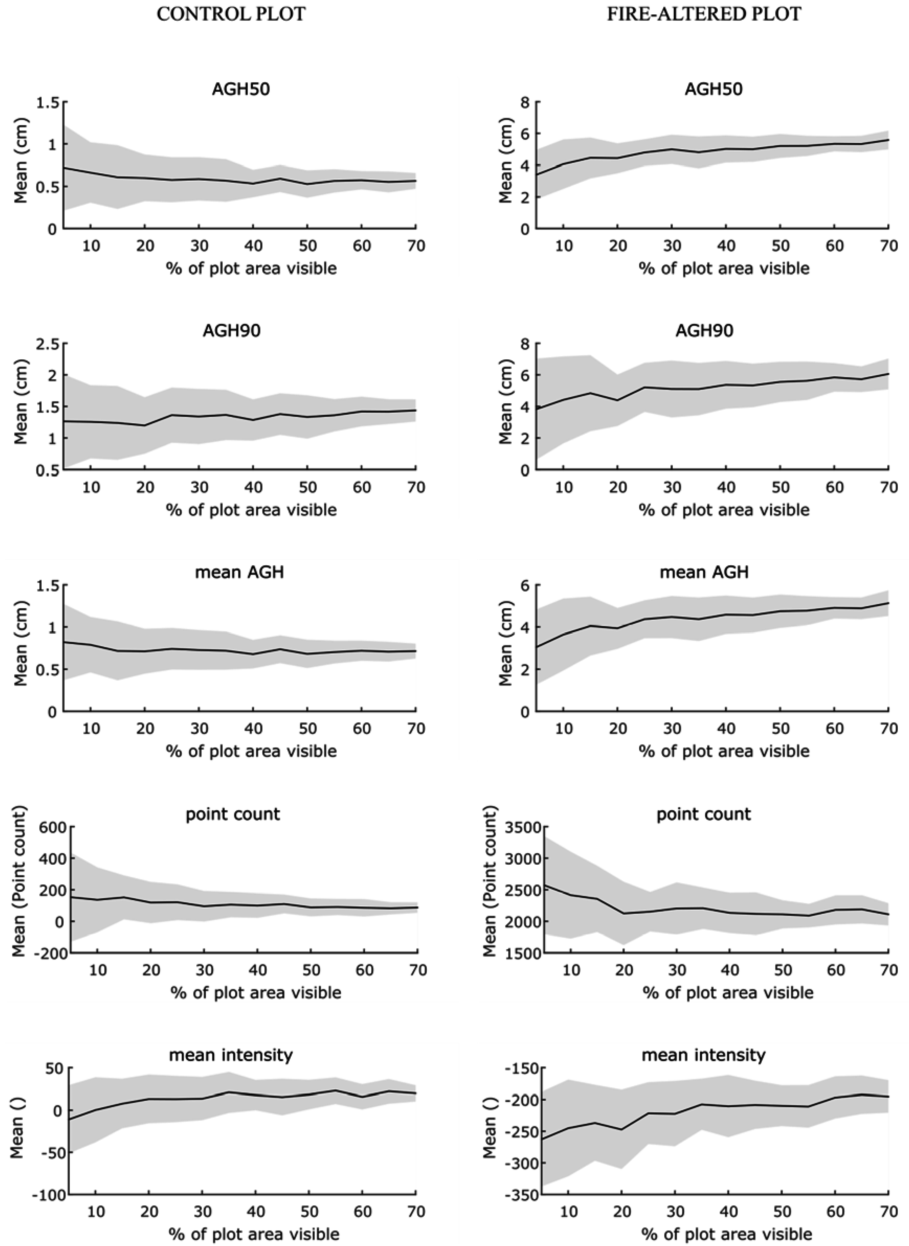
3.2.3. Effects of Occlusion

The mean value of the various AGH metrics showed very little change for the different visible plot area coverage in the control plot. As examples, the plots of AGH50, AGH90, mean AGH, point count and mean intensity are shown in Figure 7. The mean change decreased slightly from 0.008 cm at 5% plot coverage to 0.007 at 70% plot coverage using the mean AGH metric. The trend for AGH50 was similar to that of mean AGH. AGH90 showed an opposite trend of an increasing mean value from 0.012 cm at 5% plot coverage to 0.014 cm at 70% plot coverage. The point count decreased from 152 at 5% plot coverage to 88 at 70% plot coverage in the control plot (Figure 7). Mean intensity metric in contrast increased slightly from −0.10 to 0.20.

In the fire-altered plot, the change detected was relatively large compared to the control plot. The mean AGH metric increased from 0.03 cm at 5% plot coverage to 0.05 cm at 70% plot coverage. A similar trend was observed in AGH50 and AGH90 metric.

The point count decreased sharply as compared to the control plot from 2570 at 5% plot coverage to 2100 at 70% plot coverage. Mean intensity metric showed an increase just like in the control plot.

A common trend observed in both the plots was that although the mean change in value by the various metrics was very small the associated standard deviation values decreased with increasing plot area coverage. For example, the mean standard deviation values calculated using mean AGH decreased from 0.005 cm (5% plot coverage) to 0.001 cm (70% plot coverage) in the control plot and from 0.018 cm (5% plot coverage) to 0.006 cm (70% plot coverage) in the fire-altered plot. This was consistently observed across different metrics with larger standard deviation values at 5% plot coverage as compared to 70% plot coverage irrespective of the plots.

Figure 7. Mean and Standard Deviation (grey polygon) at different plot coverage for five sample metrics from the control and fire-altered plot.

Figure 7. Mean and Standard Deviation (grey polygon) at different plot coverage for five sample metrics from the control and fire-altered plot.

4. Discussion

TLS technology is increasingly being used to produce accurate measurements of forest understorey conditions [15,44,45]. However, the ability to monitor understorey forest dynamics (biomass loss or growth) using TLS has not been widely reported. Results obtained in this study indicate that fire-induced change, as an example of a disturbance in a forest understorey, is clearly discernible between multi-temporal TLS scans. The spatial distribution of change detected by most of the metrics in the fire-altered plot was found to be in agreement with visual field assessments demonstrating the concept of similarity. TLS derived metrics were assessed for correctly reporting minimal or no change in unaltered natural landscapes. In this study, this concept of stability was assessed using the control plot. All metrics showed only small changes between 1% and 5% in the control plot. The concept of sensitivity was explored by the ability of the metrics to detect fire-induced change in the forest understorey. In the fire-altered plot, all metrics (except AGH skewness_change, AGH kurtosis_change and mean intensity_change) showed a change between 30% and 52% whilst 10 of these exhibited bimodal distribution highlighting the subplot sensitivity of TLS metrics to detecting fire-induced change.

The methodology employed in this research is unique in that it applies bi-temporal TLS scans captured in single-scan mode to detect and quantify change in forest understorey. Scans were captured in single-scan mode and with a minimal fixed reference system which allowed for faster data acquisition and processing whilst also avoiding the need for co-registration [46,47]. It has been demonstrated that whilst TLS data acquired in single-scan mode suffers from some limitations such as occlusion [43], such datasets still have utility in change detection studies as has been demonstrated in this paper. However, in change detection studies in a forested environment, occlusion due to high tree densities needs to be carefully considered. The results of modelling the effects of occlusion in this paper show that high levels of occlusion are likely to bias the results towards changes occurring closer to the scanner’s location (i.e., the plot centre). Hence, for the change detection methods described in this paper using TLS to be successful, it is recommended that at least 50% plot visibility needs to be achieved.

Given that the control plot received no burn it was reasonable to expect that there would be little or no change detected between the two TLS data capture. TLS-derived metrics recorded a large change in metric values <10% voxels across the plot. The upper AGH_change percentiles (AGH90_change, AGH95_change and AGH99_change) were relatively less stable as compared to some of the lower AGH percentiles (AGH10_change to AGH50_change) (for example AGH95_change.σ = 0.21 and AGH50_change σ = 0.14) in the control plot. It could be that in the event of a low intensity change event such as prescribed burns, environmental factors such as wind can potentially affect the stability of these metrics because of movement of features in the landscape. It must be noted that during the second set of TLS data capture the conditions in the study area were extremely windy with faint drizzle which may have also contributed to noise in the point clouds. Another reason is that these upper AGH_change percentiles are also most likely to contain change in response to phenological growth and senescence in the control plot. However, the histogram distribution for some lower AGH_change percentiles (AGH10_change to AGH40_change) was multimodal while for the other metrics it was normal. These lower AGH_change percentile metrics are likely to be affected by interaction with ground elements and thus may not be appropriate for describing unaltered understorey landscapes.

In the fire-altered plot, 16 TLS-derived metrics were reported as being sensitive at detecting fire-induced change in the forest understorey. This is supported by the σ values being much larger in the fire-altered plot (0.32–1.67) in comparison to the control plot (0.14–0.45) as listed in Table 3. A larger σ value is representative of unburnt patches interspersed with burnt areas in the fire-altered plot when examining the histograms. Histograms of AGH_change percentiles such as AGH30_change to AGH95_change exhibit bimodal distributions with peaks in the range of 0.3–0.5 and 0.8–1.1 in the fire-altered plot. The local maximum peak between 0.3 and 0.5 corresponds to voxels that have undergone fire-induced change. These voxels are also found to lie outside the dashed red line in Figure 5 which is indicative of a fire-induced change. Similarly, voxels around the local maximum peak centred at 0.8–1.1 are those belonging to unburnt patches in the forest understorey in the fire-altered plot. As stated earlier, values closer to 1 in ratio-based metrics is indicative of little or no change. Thus, the bimodal distribution exhibited by some TLS-derived metrics is able to account for populations belonging to two disparate groups. In this research these two groups would be burnt and unburnt forest understorey. The upper AGH_change percentiles (AGH70_change to AGH99_change) and maximum AGH_change are shown to record a lower fire-induced change (37%–53% voxels) as compared to lower AGH_change percentiles (62%–67% voxels). The field based assessments recorded burn in 60%–70% of the plot area. This could be attributed to the environmental conditions (e.g. wind) and patchy nature of prescribed burns. If a voxel with dimensions 0.5 × 0.5 ×1.0 m was affected by fire, a few remaining stalks of grass may classify this voxel as being unburnt. These findings suggest that the upper AGH_change percentiles may not actually be appropriate for reporting fire-induced change following low intensity prescribed burns. The mean intensity_change metric which was stable in the control plot showed a change in the fire-altered plot. The change recorded was only 19% which suggests that the change detected by mean intensity_change in the fire-altered plot could be due to a number of factors other than fire.

Although it has been established in this paper that TLS technology and its derived metrics are sensitive at detecting fire-induced change in forested understorey, it is equally important to attempt to map where these changes have occurred on the ground. The patchy nature of prescribed burns is a well acknowledged fact [3]. As shown in Figure 6, vast areas of the control plot recorded no change which was to be expected. However, the majority of the change detected in the control plot for most metrics was found to occur in a small localised area of the plot. This corresponded and could be explained due to the defoliation of a fallen tree. However, this change was not detected by AGH99_change, mode AGH_change and maximum AGH_change metrics as the large woody component of the tree was still present. This defoliation appears to present a similar pattern to fire induced change within the fire-altered plot where large woody debris was still present following prescribed burns. Whilst it was ascertained that the ideal metric should remain stable and detect little or no-change in the control plot, it would be inaccurate if the metric did not detect a real and a substantial non fire-induced change in the forest understorey even in the undisturbed plot.

In the fire-altered plot, unburnt patches interspersed with burnt patches are reported by the majority of the metrics (except AGH skewness_change and AGH kurtosis_change). Figure 4A shows an image from the fire-altered plot highlighting the mosaic landscape as a result of the prescribed burn. Although the degree of patchiness and plot area burnt is extremely variable amongst the metrics (22%–71%), the ability of TLS technology to map this “patchiness” is an extremely promising finding. The level of patchiness within burnt areas can determine the proportion of vegetation population exposed to heat. This can inform vegetation mortality rates and seed germination [48,49]. Patchiness can also help predict fire intensity. Low intensity fires are shown to be significantly patchier than higher intensity fires [50]. The pattern of the burn represented by the binary maps (Figure 6) for many metrics (AGH10_change to AGH50_change, mean AGH_change and point count_change) is similar and closer to the field assessments of burnt areas. This includes both the percentage area burnt and spatial distribution of burnt areas in the fire-altered plot. These metrics consistently detected a much larger burnt area on the eastern side of the plot (Figure 4B) in comparison to the west with a large unburnt patch in the southwest region of the plot.

From the above analysis AGH50_change, mean AGH_change and point count_change seem to be the most suitable individual metrics for attributing change in an altered understorey forest whilst remaining stable in an undisturbed one. It is important to ensure that the metrics being used in change detection studies remain stable in an undisturbed landscape whilst remaining sensitive at attributing change in an altered landscape. It is also important to consider that the metrics being used report spatial distribution of change similar to change occurring on the ground. These findings suggest that TLS technology and TLS-derived metrics can be used to supplement the routine qualitative field assessments of change which are often based on visual estimates thereby providing a method to allow for a more quantified and accurate reporting approach. The burn maps showing the spatial distribution of change can be used by land managers to identify areas in need of urgent rehabilitation.

Future work could involve exploring the utility of the method presented in this research to quantify biomass change. This research could be further developed by exploring the binary change detection maps for mapping different burn severity levels. This could also help identify unburnt patches which can help in understanding ecological impacts on fire-sensitive plants, watershed hydrology and soil stability amongst others. This may involve using a combination of the metrics used in this paper given their demonstrated differences in each metric shown here. Given that post-burn TLS scans were carried out within two weeks of the burn event, they helped ascertain change in the landscape in response to the burn. A longitudinal study involving multi-temporal scans over longer time scales can help monitor fuel accumulation, post-fire regeneration dynamics and vegetation senescence.

5. Conclusions

The objective of this paper was to assess a set of terrestrial LiDAR-derived metrics for detecting, analysing and visualising fire-induced change in a forest understorey following low intensity prescribed burns. The metrics were assessed in their ability to remain stable in unaltered natural landscape whilst being sensitive enough to detect fire-induced understorey change. They were also assessed for their similarity in mapping the spatial distribution of change and percentage area burnt based on visual field assessments. The key findings of this research demonstrate that terrestrial LiDAR technology can be effectively used in a single-scan mode to make repeated measurements in both an unaltered and altered forest understorey with a minimal fixed reference system. Three TLS-derived metrics AGH50_change (change in Above Ground Height at 50th percentile), mean AGH_change (change in mean Above Ground Height) and point count_change are capable of attributing fire-induced change in forest understorey that can be qualitatively validated with field assessments. These metrics whilst detecting fire-induced change (sensitive) are also capable of capturing the patchy nature of prescribed burns and produce burn maps comparable to visual field assessments of area burnt (similarity). At the same time, these three metrics report little or no change in an undisturbed (control plot) forest understorey (stable). The method described in this paper facilitates rapid data capture, easy post-processing of data and is fit-for-purpose in terms of the required accuracies to detect fire-induced changes in forest understorey. This approach has great potential for land and forest managers to quantitatively monitor dynamic changes in the understorey landscape in a way that is repeatable and accurate. Given the change agent in this research was a low intensity prescribed burn, it is encouraging to note that Terrestrial LiDAR technology and some of the metrics show immense potential in attributing and mapping subtle fire-induced changes. In the event of large-scale environmental changes (e.g., wildfires or floods), mapping change in forested understorey using such techniques can potentially assist land managers in identifying areas in need of urgent rehabilitation, accurately quantify the area of land affected and fuel management.

References

1. Roy, D.P.; Lewis, P.E.; Justice, C.O. Burned area mapping using multi-temporal moderate spatial resolution data—A bi-directional reflectance model-based expectation approach. Remote Sens. Environ. 2002, 83, 263–286. [Google Scholar] [CrossRef]
2. Gill, A.M. Fire and the Australian flora: A review. Aust. For. 1975, 38, 4–25. [Google Scholar] [CrossRef]
3. Penman, T.D.; Kavanagh, R.P.; Binns, D.L.; Melick, D.R. Patchiness of prescribed burns in dry sclerophyll eucalypt forests in South-eastern Australia. For. Ecol. Manag. 2007, 252, 24–32. [Google Scholar] [CrossRef]
4. Fernandes, P.M.; Botelho, H.S. A review of prescribed burning effectiveness in fire hazard reduction. Int. J. Wildland Fire 2003, 12, 117–128. [Google Scholar] [CrossRef]
5. Leigh, J.H.; Noble, J.C. The role of fire in the management of rangelands in Australia. In Fire and the Australian Biota; Grove, R.H., Noble, I.R., Eds.; Australian Academy of Science: Canberra, Australia, 1981; pp. 471–495. [Google Scholar]
6. Victorian Lands Alliance. Fuel Reduction Burning in Southern Australia’s Forests: A Review of Its Effectiveness as a Bushfire Management Tool 2010; Victorian Lands Alliance: Benalla, VIC, Australia, 2010. Available online: http://www.royalcommission.vic.gov.au/Documents/Document-files/Exhibits/SUBM-002-055-0031_R.pdf (accessed on 9 February 2015).
7. Robichaud, P.R. Post-fire stabilization and rehabilitation. In Fire Effects on Soils and Restoration Strategies; Robichaud, P.R., Ed.; CRC Press: Boca Raton, FL, USA, 2009; pp. 299–320. [Google Scholar]
8. Wittenberg, L.; Malkinson, D.; Beeri, O.; Halutzy, A.; Tesler, N. Spatial and temporal patterns of vegetation recovery following sequences of forest fires in a Mediterranean landscape, Mt. Carmel Israel. Catena 2007, 71, 76–83. [Google Scholar] [CrossRef]
9. Lentile, L.B.; Morgan, P.; Hudak, A.T.; Bobbitt, M.J.; Lewis, S.A.; Smith, A.; Robichaud, P.R. Post-fire burn severity and vegetation response following eight large wildfires across the western United States. Fire Ecol. 2007, 3, 91–108. [Google Scholar] [CrossRef]
10. Boby, L.A.; Schuur, E.A.G.; Mack, M.C.; Verbyla, D.; Johnstone, J.F. Quantifying fire severity, carbon, and nitrogen emissions in Alaska’s boreal forest. Ecol. Appl. 2010, 20, 1633–1647. [Google Scholar] [CrossRef] [PubMed]
11. Key, C.H.; Benson, N.C. Landscape assessment: Ground measure of severity, the Composite Burn Index; and remote sensing of severity, the Normalized Burn Ratio. In FIREMON: Fire Effects Monitoring and Inventory System; Lutes, D.C., Lutes, D.C., Keane, R.E., Caratti, J.F., Key, C.H., Benson, N.C., Gangi, L.J., Eds.; USDA Forest Service, Rocky Mountain Research Station: Ogden, UT, USA, 2005. [Google Scholar]
12. DSE. Remote Sensing of Fire Severity for Prescribed Burns: Field Assessment; Department of Sustainability and Environment: Melbourne, Australia, 2010.
13. Hudak, A.T.; Evans, J.S.; Stuart Smith, A.M. LiDAR utility for natural resource managers. Remote Sens. 2009, 1, 934–951. [Google Scholar] [CrossRef]
14. Jakubowski, M.K.; Guo, Q.; Collins, B.; Stephens, S.; Kelly, M. Predicting Surface fuel models and fuel metrics using Lidar and CIR imagery in a dense, mountainous forest. Photogramm. Eng. Remote Sens. 2013, 79, 37–49. [Google Scholar] [CrossRef]
15. Loudermilk, E.L.; Hiers, J.K.; O’Brien, J.J.; Mitchell, R.J.; Singhania, A.; Fernandez, J.C.; Cropper, W.P.; Slatton, K.C. Ground-based LiDAR: A novel approach to quantify fine-scale fuelbed characteristics. Int. J. Wildland Fire 2009, 18, 676–685. [Google Scholar] [CrossRef]
16. Riano, D.; Meier, E.; Allgower, B.; Chuvieco, E.; Ustin, S.L. Modeling airborne laser scanning data for the spatial generation of critical forest parameters in fire behavior modeling. Remote Sens. Environ. 2003, 86, 177–186. [Google Scholar] [CrossRef]
17. Rowell, E.; Seielstad, C. Characterising grass, litter, and shrub fuels in longleaf pine forest pre- and post-fire using terrestrial LiDAR. In Proceedings of SilviLaser 2012, Vancouver, BC, Canada, 16–18 September 2012.
18. Martinuzzi, S.; Vierling, L.A.; Gould, W.A.; Falkowski, M.J.; Evans, J.S.; Hudak, A.T.; Vierling, K.T. Mapping snags and understory shrubs for a LiDAR-based assessment of wildlife habitat suitability. Remote Sens. Environ. 2009, 113, 2533–2546. [Google Scholar] [CrossRef]
19. Muukkonen, P.; Makipaa, R. Empirical biomass models of understorey vegetation in boreal forests according to stand and site attributes. Boreal Environ. Res. 2006, 11, 355–369. [Google Scholar]
20. Dubayah, R.O.; Drake, J.B. LiDAR remote sensing for forestry. J. For. 2000, 98, 44–46. [Google Scholar]
21. Kane, V.R.; McGaughey, R.J.; Bakker, J.D.; Gersonde, R.F.; Lutz, J.A.; Franklin, J.F. Comparisons between field-and LiDAR-based measures of stand structural complexity. Can. J. For. Res. 2010, 40, 761–773. [Google Scholar] [CrossRef]
22. Lefsky, M.A.; Cohen, W.B.; Acker, S.A.; Spies, T.A.; Parker, G.G.; Harding, D.J. LiDAR remote sensing of forest canopy structure and related biophysical parameters at H.J. Andrews Experimental Forest, Oregon, USA. In Natural Resources Management Using Remote Sensing and GIS; ASPRS: Washington, DC, USA, 1997; pp. 79–91. [Google Scholar]
23. Lefsky, M.A.; Hudak, A.T.; Cohen, W.B.; Acker, S.A. Patterns of covariance between forest stand and canopy structure in the Pacific Northwest. Remote Sens. Environ. 2005, 95, 517–531. [Google Scholar] [CrossRef]
24. Means, J.E.; Acker, S.A.; Fitt, B.J.; Renslow, M.; Emerson, L.; Hendrix, C.J. Predicting forest stand characteristics with airborne scanning LiDAR. Photogramm. Eng. Remote Sens. 2000, 66, 1367–1371. [Google Scholar]
25. Meyer, V.; Saatchi, S.S.; Chave, J.; Dalling, J.; Bohlman, S.; Fricker, G.A.; Robinson, C.; Neumann, M. Detecting tropical forest biomass dynamics from repeated airborne LiDAR measurements. Biogeosci. Discuss 2013, 10, 1957–1992. [Google Scholar] [CrossRef]
26. Naesset, E. Determination of mean tree height of forest stands using airborne laser scanner data. ISPRS J. Photogramm. Remote Sens. 1997, 52, 49–56. [Google Scholar] [CrossRef]
27. Watt, P.J.; Donoghue, D.N.M.; Dunford, R.W. Forest parameter extraction using terrestrial laser scanning. In Proceedings of ScandLaser Scientific Workshop on Airborne Laser Scanning of Forests, Umea, Sweden, 2–4 September 2003; pp. 237–244.
28. Bienert, A.; Scheller, S.; Keane, E.; Mohan, F.; Nugent, C. Tree detection and diameter estimations by analysis of forest terrestrial laser scanner point clouds. In Proceedings of SilviLaser 2007, Espoo, Finland, 12–14 September 2007.
29. Watt, P.J.; Donoghue, D.N.M. Measuring forest structure with terrestrial laser scanning. Int. J. Remote Sens. 2005, 26, 1437–1446. [Google Scholar] [CrossRef]
30. Moskal, L.M.; Zheng, G. Retrieving forest inventory variables with terrestrial laser scanning (TLS) in urban heterogeneous forest. Remote Sens. 2011, 4, 1–20. [Google Scholar] [CrossRef]
31. Huang, P.; Pretzsch, H. Using terrestrial laser scanner for estimating leaf areas of individual trees in a conifer forest. Trees 2010, 24, 609–619. [Google Scholar] [CrossRef]
32. Jupp, D.L.B.; Culvenor, D.S.; Lovell, J.L.; Newnham, G.J.; Strahler, A.H.; Woodcock, C.E. Estimating forest LAI profiles and structural parameters using a ground-based laser called “Echidna®”. Tree Physiol. 2009, 29, 171–181. [Google Scholar] [CrossRef] [PubMed]
33. Danson, F.M.; Hetherington, D.; Morsdorf, F.; Koetz, B.; Allgower, B. Forest canopy gap fraction from terrestrial laser scanning. IEEE Geosci. Remote Sens. Lett. 2007, 4, 157–160. [Google Scholar] [CrossRef] [Green Version]
34. Liang, X.; Hyyppä, J.; Kaartinen, H.; Holopainen, M.; Melkas, T. Detecting changes in forest structure over time with bi-temporal terrestrial laser scanning data. ISPRS Int. J. Geo-Inf. 2012, 1, 242–255. [Google Scholar] [CrossRef]
35. Xiao, W.; Xua, S.; Elberinka, S.O.; Vosselmana, G. Change detection of trees in urban areas using mutil-temporal airborne LiDAR point clouds. Proc. SPIE 2012. [Google Scholar] [CrossRef]
36. Yu, X.; Hyyppä, J.; Kaartinen, H.; Maltamo, M. Automatic detection of harvested trees and determination of forest growth using airborne laser scanning. Remote Sens. Environ. 2004, 90, 451–462. [Google Scholar] [CrossRef]
37. Wallace, L.O.; Watson, C.; Lucieer, A. Detecting pruning of individual stems using airborne laser scanning data captured from an unmanned aerial vehicle. Int. J. Appl. Earth Obs. Geoinf. 2014, 30, 76–85. [Google Scholar] [CrossRef]
38. Goodwin, N.R. Assessing Understorey Structural Characteristics in Eucalypt Forests: An Investigation of LiDAR Techniques. Ph.D. Thesis, University of New South Wales, Sydney, Australia, 2006. [Google Scholar]
39. Wang, C.; Glenn, N.F. Estimation of fire severity using pre-and post-fire LiDAR data in sagebrush steppe rangelands. Int. J. Wildland Fire 2009, 18, 848–856. [Google Scholar] [CrossRef]
40. Wing, B.M.; Ritchie, M.W.; Boston, K.; Cohen, W.B.; Gitelman, A.; Olsen, M.J. Prediction of understory vegetation cover with airborne LiDAR in an interior ponderosa pine forest. Remote Sens. Environ. 2012, 124, 730–741. [Google Scholar] [CrossRef]
41. Hines, F.; Tolhurst, K.; Wilson, A.; McCarthy, G. Overall Fuel Hazard Assessment Guide; Fire and Adaptive Management. Department of Sustainability and Environment: Melbourne, Australia, 2010. [Google Scholar]
42. Isenburg, M.; Schewchuck, J. LAStools: Converting, Viewing and Compressing LiDAR Data in LAS Format. Available online: http://www.cs.unc.edu/~isenburg/lastools/ (accessed on 13 May 2015).
43. Dassot, M.; Constant, T.; Fournier, M. The use of terrestrial LiDAR technology in forest science: Application fields, benefits and challenges. Ann. For. Sci. 2011, 68, 959–974. [Google Scholar] [CrossRef]
44. Vierling, L.A.; Xu, Y.; Eitel, J.U.H.; Oldow, J.S. Shrub characterization using terrestrial laser scanning and implications for airborne LiDAR assessment. Can. J. Remote Sens. 2013, 38, 709–722. [Google Scholar] [CrossRef]
45. Olsoy, P.J.; Glenn, N.F.; Clark, P.E. Estimating sagebrush biomass using terrestrial laser scanning. Rangel. Ecol. Manag. 2014, 67, 224–228. [Google Scholar] [CrossRef]
46. Liang, X.; Litkey, P.; Hyyppa, J.; Kaartinen, H.; Vastaranta, M.; Holopainen, M. Automatic stem mapping using single-scan terrestrial laser scanning. IEEE Trans. Geosci. Remote Sens. 2012, 50, 661–670. [Google Scholar] [CrossRef]
47. Litkey, P.; Liang, X.; Kaartinen, H.; Hyyppä, J.; Kukko, A.; Holopainen, M. Single-scan TLS methods for forest parameter retrieval. In Proceedings of the 8th SilviLaser 2008, Edinburgh, UK, 17–19 September 2008.
48. Turner, M.G.; Hargrove, W.W.; Gardner, R.H.; Romme, W.H. Effects of fire on landscape heterogeneity in Yellowstone National Park, Wyoming. J. Veg. Sci. 1994, 5, 731–742. [Google Scholar] [CrossRef]
49. Price, O.; Russell-Smith, J.; Edwards, A. Fine-scale patchiness of different fire intensities in sandstone heath vegetation in northern Australia. Int. J. Wildland Fire 2003, 12, 227–236. [Google Scholar] [CrossRef]
50. OoI, M.K.; Whelan, R.J.; Auld, T.D. Persistence of obligate-seeding species at the population scale: Effects of fire intensity, fire patchiness and long fire-free intervals. Int. J. Wildland Fire 2006, 15, 261–269. [Google Scholar] [CrossRef]