
A Polarimetric First-Order Model of Soil Moisture Effects on the DInSAR Coherence

Abstract
:
1. Introduction
2. Proposed Model
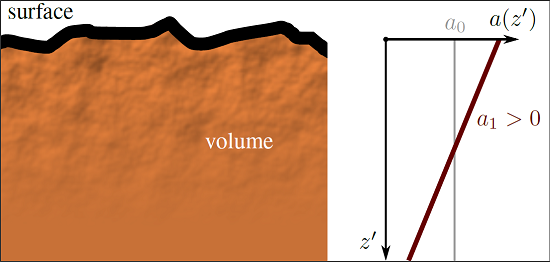
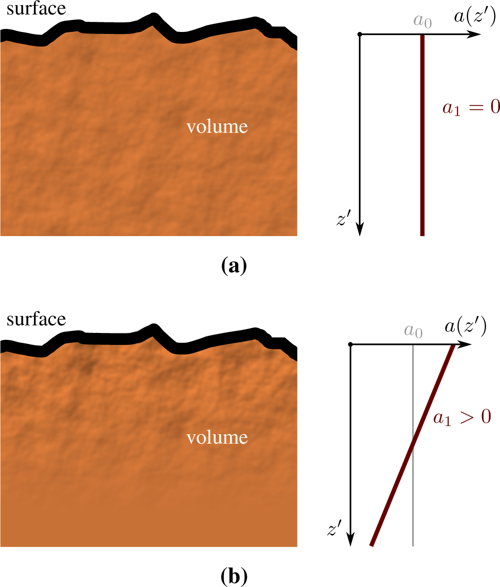
2.1. Permittivity Fluctuations
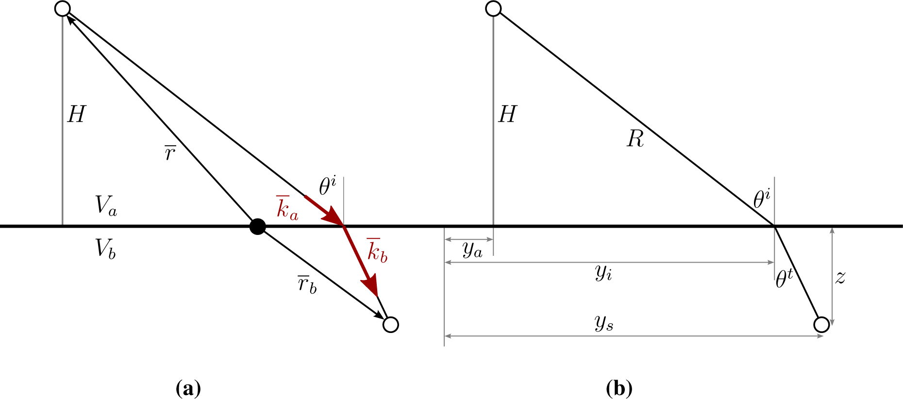
2.2. Surface Term
2.3. Propagation Phase
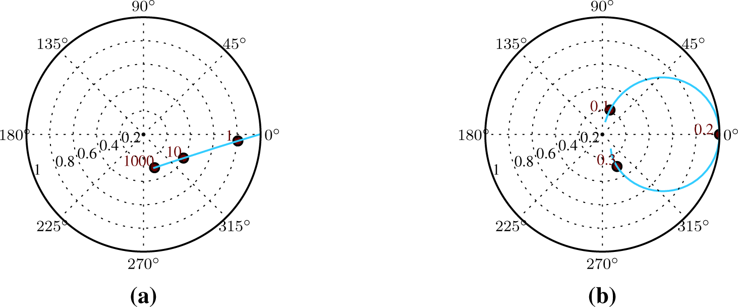
2.4. Interferometric Observables
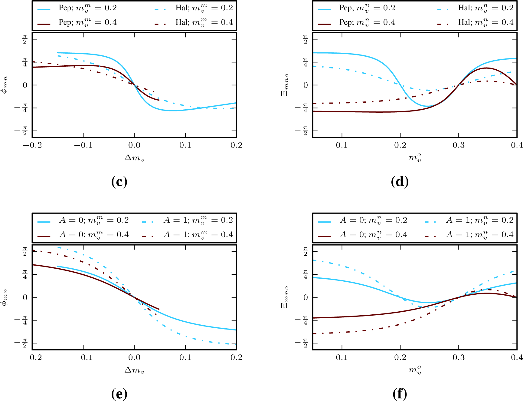
2.5. Parametric Solutions
3. Calibration and Model Assessment
3.1. Study Site and Data
3.1.1. Study Site
3.1.2. Soil Moisture Data
3.1.3. Radar Data and Processing
3.2. Rationale
3.3. Minimization of Misfit
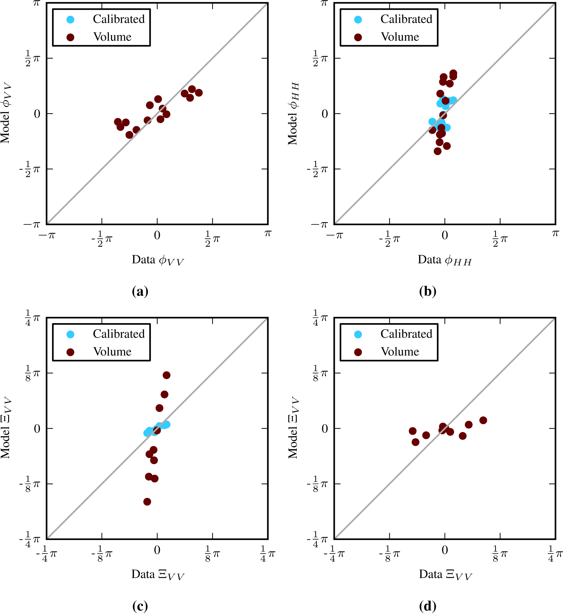
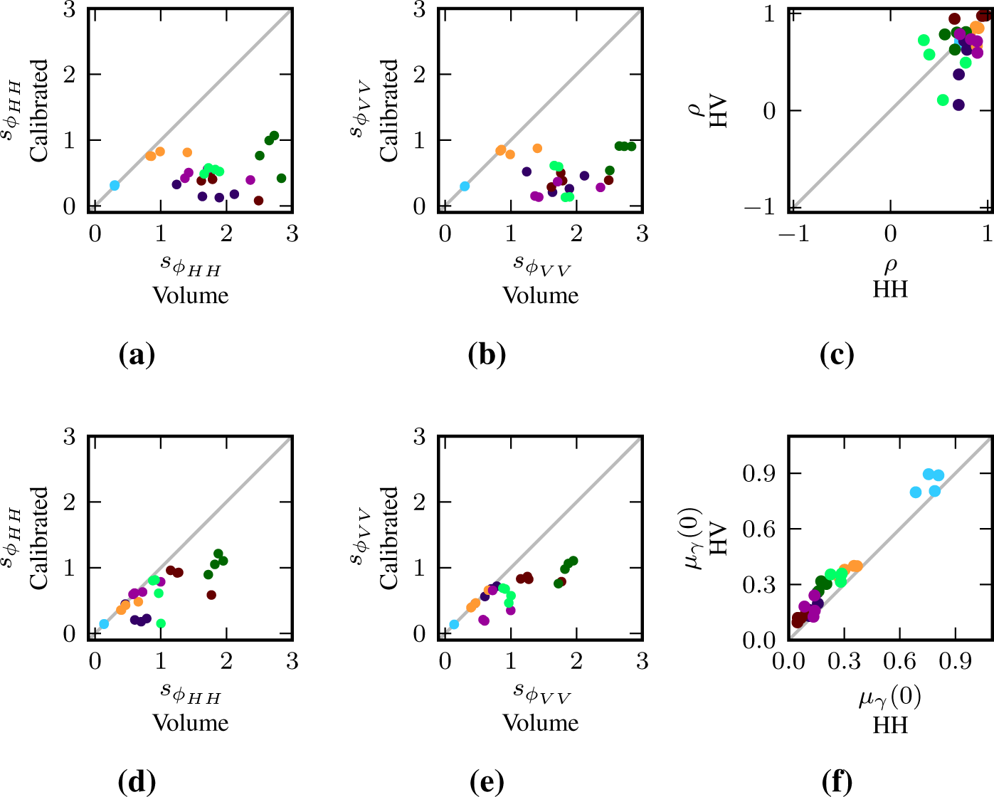
3.4. Evaluation
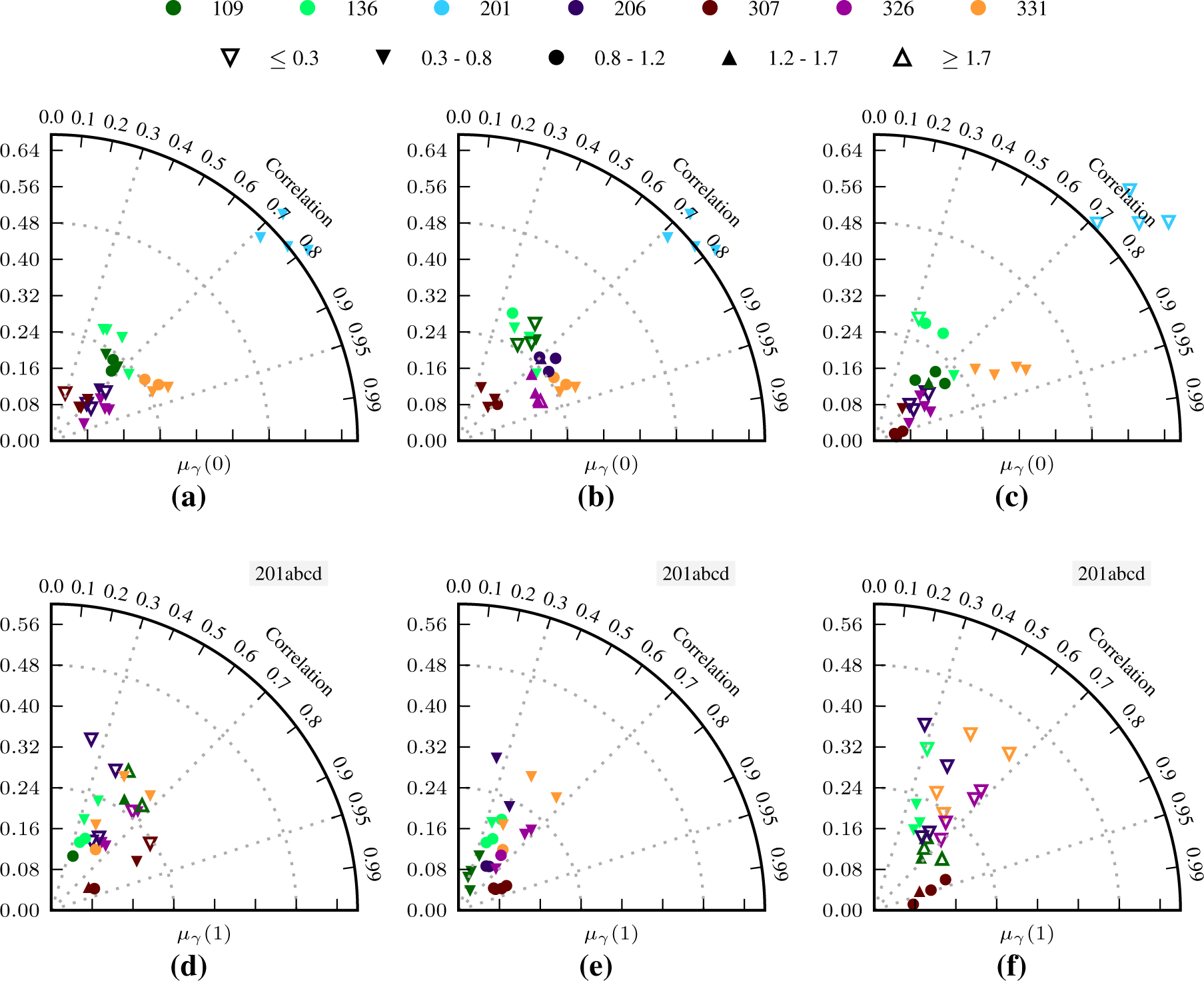
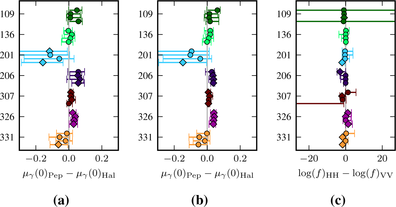
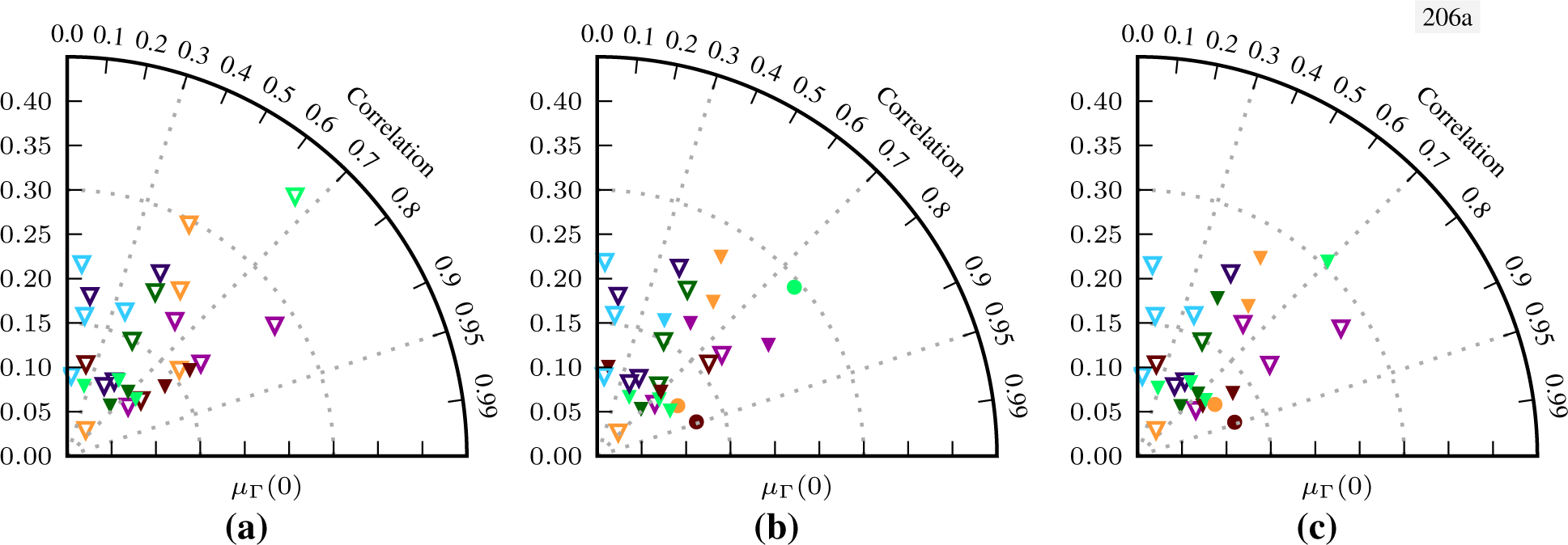
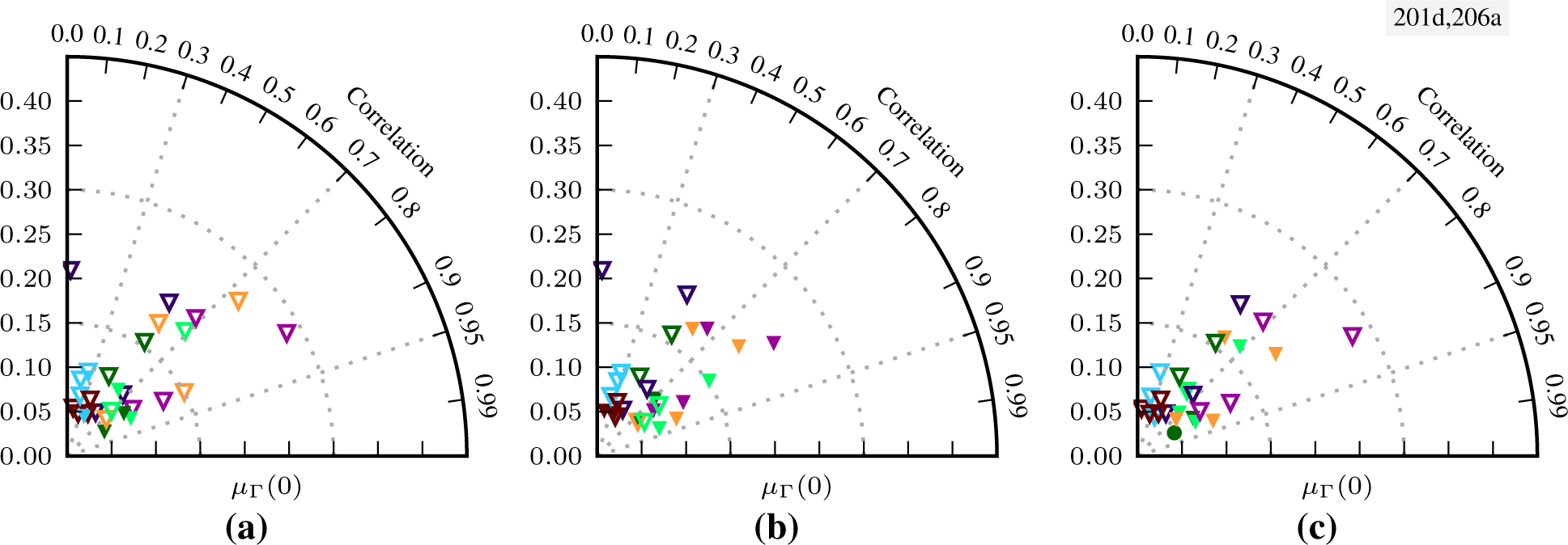
4. Results
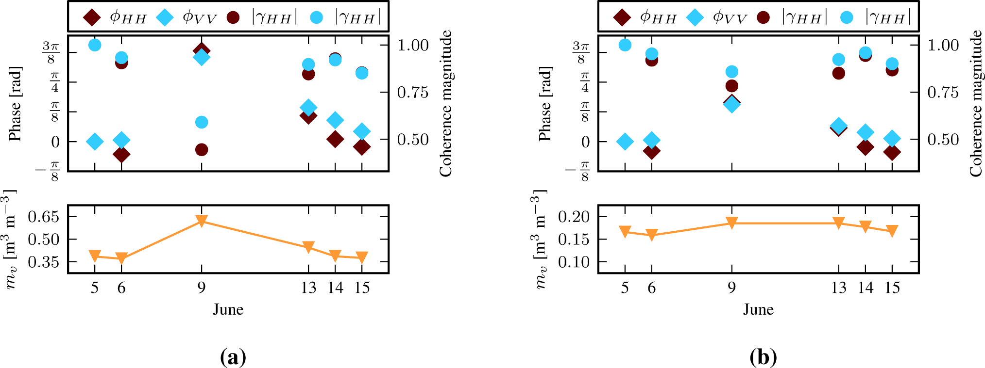
4.1. Examples
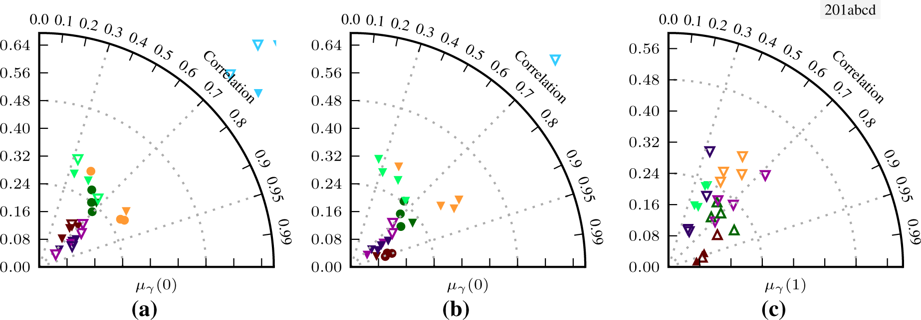
4.2. Coherence
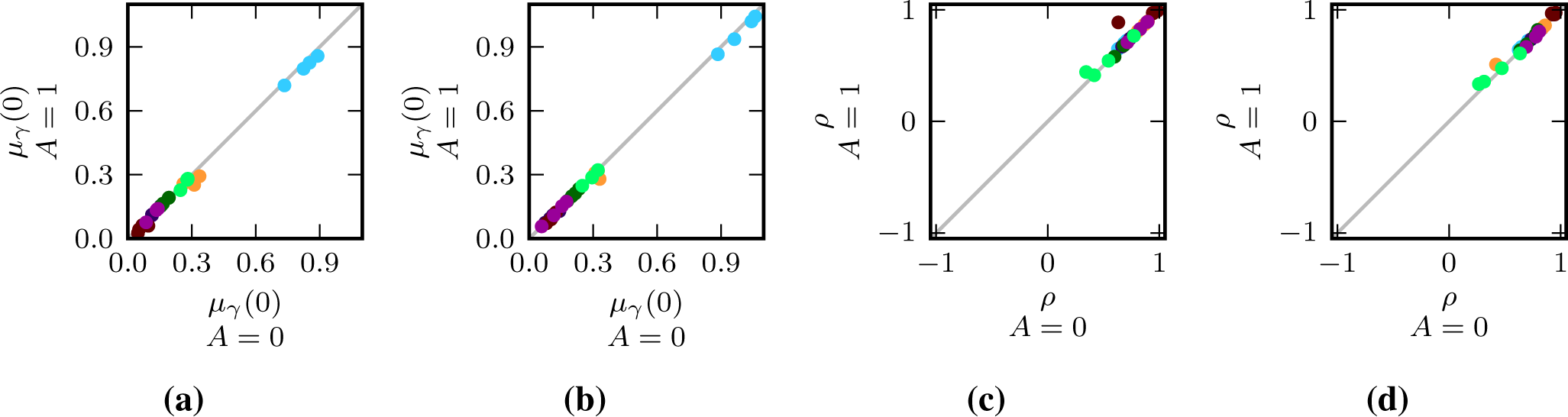
4.2.1. Calibration with A = 0
4.2.2. Calibration with A = 1
4.3. Bicoherence
5. Discussion
5.1. Polarimetry
5.2. Parameterization and Uncertainties of Soil Moisture Dependence
5.3. Extensions and Underdetermination
6. Conclusions
Supplementary Data
remotesensing-07-07571-s001.pdfAcknowledgments
Author Contributions
Conflicts of Interest
References
- Bamler, R.; Hartl, P. Synthetic aperture radar interferometry. Inverse Probl 1998, 14, 1–54. [Google Scholar]
- Gabriel, A.; Goldstein, R.; Zebker, H. Mapping small elevation changes over large areas: Differential radar interferometry. J. Geophys. Res 1989, 94, 9183–9191. [Google Scholar]
- Nolan, M. DInSAR measurement of soil moisture. IEEE Trans. Geosci. Remote Sens 2003, 41, 2802–2813. [Google Scholar]
- Barrett, B.; Whelan, P.; Dwyer, E. Detecting changes in surface soil moisture content using differential SAR interferometry DInSAR. Int. J. Remote Sens 2013, 34, 7091–7112. [Google Scholar]
- Rudant, J.P.; Bedidi, A.; Calonne, R.; Massonnet, D.; Nesti, G.; Tarchi, D. Laboratory experiment for the interpretation of phase shift in SAR interferograms. Proceedings of FRINGE, Zurich, Switzerland, 30 September 1996.
- Morrison, K.; Bennett, J.; Nolan, M.; Menon, R. Laboratory measurement of the DInSAR response to spatiotemporal variations in soil moisture. IEEE Trans. Geosci. Remote Sens 2011, 49, 3815–3823. [Google Scholar]
- Zwieback, S.; Hensley, S.; Hajnsek, I. Assessment of soil moisture effects on L-band radar interferometry. Remote Sens. Environ 2015, 164, 77–89. [Google Scholar]
- Nolan, M. Penetration depth as a DInSAR observable and proxy for soil moisture. IEEE Trans. Geosci. Remote Sens 2003, 41, 532–537. [Google Scholar]
- Rabus, B.; Wehn, H.; Nolan, M. The importance of soil moisture and soil structure for InSAR phase and backscatter, as determined by FDTD modeling. IEEE Trans. Geosci. Remote Sens 2010, 48, 2421–2429. [Google Scholar]
- De Zan, F.; Parizzi, A.; Prats-Iraola, P.; Lopez-Dekker, P. A SAR interferometric model for soil moisture. IEEE Trans. Geosci. Remote Sens 2014, 52, 418–425. [Google Scholar]
- Yin, Q.; Hong, W.; Li, Y.; Lin, Y. Analysis on soil moisture estimation of SAR data based on coherent scattering model. Proceedings of the EUSAR, Berlin, Germany, 3–5 June 2014.
- Jackson, J. Classical Electrodynamics, 3rd ed; John Wiley & Sons: Hoboken, NJ, USA, 1999. [Google Scholar]
- Zwieback, S.; Bartsch, A.; Melzer, T.; Wagner, W. Probablistic fusion of Ku and C band scatterometer data for determining the Freeze/Thaw State. IEEE Trans. Geosci. Remote Sens 2012, 50, 2583–2594. [Google Scholar]
- Mironov, V.; Savin, I. A temperature-dependent multi-relaxation spectroscopic dielectric model for thawed and frozen organic soil at 0.05–15 GHz. Phys. Chem. Earth Parts A/B/C 2015, in press. [Google Scholar]
- Hallikainen, M.; Ulaby, F.; Dobson, M.; El-Rayes, M.; Wu, L.K. Microwave dielectric behavior of wet soil–Part I: Empirical models and experimental observations. IEEE Trans. Geosci. Remote Sens 1985, 23, 25–34. [Google Scholar]
- Peplinski, N.R.; Ulaby, F.T.; Dobson, M.C. Dielectric properties of soils in the 0.3–1.3-GHz range. IEEE Trans. Geosci. Remote Sens 1995, 33, 803–807. [Google Scholar]
- Tsang, L.; Kong, J.A.; Ding, K.H. Scattering of Electromagnetic Waves: Theories and Applications; John Wiley & Sons: Hoboken, NJ, USA, 2000. [Google Scholar]
- Cloude, S.R. Polarisation: Applications in Remote Sensing; Oxford University Press: Oxford, UK, 2009. [Google Scholar]
- Rice, S.O. Reflection of electromagnetic waves from slightly rough surfaces. Commun. Pure Appl. Math 1951, 4, 351–378. [Google Scholar]
- Yamaguchi, Y.; Moriyama, T.; Ishido, M.; Yamada, H. Four-component scattering model for polarimetric SAR image decomposition. IEEE Trans. Geosci. Remote Sens 2005, 43, 1699–1706. [Google Scholar]
- Hajnsek, I.; Jagdhuber, T.; Schoen, H.; Papathanassiou, K. Potential of estimating soil moisture under vegetation cover by means of PolSAR. IEEE Trans. Geosci. Remote Sens 2009, 47, 442–454. [Google Scholar]
- Treuhaft, R.; Cloude, S.R. The structure of oriented vegetation from polarimetric interferometry. IEEE Trans. Geosci. Remote Sens 1999, 37, 2620–2624. [Google Scholar]
- Ishimaru, A. Wave Propagation and Scattering in Random Media; IEEE Press: Hoboken, NJ, USA, 1997. [Google Scholar]
- Dall, J. InSAR elevation bias caused by penetration into uniform volumes. IEEE Trans. Geosc. Remote Sens 2007, 45, 2319–2324. [Google Scholar]
- Oveisgharan, S.; Zebker, H. Estimating snow accumulation from InSAR correlation observations. IEEE Trans. Geosc. Remote Sens 2007, 45, 10–20. [Google Scholar]
- Gatelli, F.; Guarnieri, A.; Parizzi, F.; Pasquali, P.; Prati, C.; Rocca, F. The Wavenumber Shift in SAR Interferometry. IEEE Trans. Geosc. Remote Sens 1994, 32, 855–865. [Google Scholar]
- Cloude, S.R. Polarization coherence tomography. Radio Sci 2006, 41. [Google Scholar] [CrossRef]
- Monnier, J.D. Phases in interferometry. New Astron. Rev 2007, 51, 604–616. [Google Scholar]
- Monnier, J. An introduction to closure phases. In Principles of Long Baseline Interferometry; Lawson, P., Ed.; JPL: La CaÃśada Flintridge, CA, USA, 1999. [Google Scholar]
- Lannes, A. Remarkable algebraic structures of phase-closure imaging and their algorithmic implications in aperture synthesis. J. Opt. Soc. Am. A 1990, 7, 500–512. [Google Scholar]
- Abramowitz, M.; Stegun, I.A. Handbook of Mathematical Functions with Formulas, Graphs, and Mathematical Tables, 9th ed; Dover: New York, NY, USA, 1964. [Google Scholar]
- Magagi, R.; Berg, A.; Goita, K.; Belair, S.; Jackson, T.; Toth, B.; Walker, A.; McNairn, H.; O’Neill, P.; Moghaddam, M.; et al. Canadian experiment for soil moisture in 2010 (CanEx-SM10): overview and preliminary results. IEEE Trans. Geosci. Remote Sens 2013, 51, 347–363. [Google Scholar]
- CanEx-SM10. Experimental Plan. Available online: http://canex-sm10.espaceweb.usherbrooke.ca/Experimental_plan_CANEx-SM10.pdf accessed on 16 March 2015.
- Jones, C.; Davis, B. High resolution Radar for response and recovery: Monitoring containment booms in Barataria Bay. Photogammetric Eng. Remote Sens 2011, 77, 102–105. [Google Scholar]
- DiCiccio, T.; Efron, B. Bootstrap confidence Intervals. Stat. Sci 1996, 11, 189–228. [Google Scholar]
- Hajnsek, I.; Pottier, E.; Cloude, S. Inversion of surface parameters from polarimetric SAR. IEEE Trans. Geosci. Remote Sens 2003, 41, 727–744. [Google Scholar]
- Oh, Y.; Sarabandi, K.; Ulaby, F. Semi-empirical model of the ensemble-averaged differential Mueller matrix for microwave backscattering from bare soil surfaces. IEEE Trans. Geosci. Remote Sens 2002, 40, 1348–1355. [Google Scholar]
- Entekhabi, D.; Rechle, R.; Koster, R.; Crow, W. Performance metrics for soil moisture retrievals and application requirements. J. Hydrometeor 2010, 11, 832–840. [Google Scholar]
- Liu, Y.; Dorigo, W.; Parinussa, R.; de Jeu, R.; Wagner, W.; McCabe, M.; Evans, J.; van Dijk, A. Trend-preserving blending of passive and active microwave soil moisture retrievals. Remote Sens. Environ 2012, 123, 280–297. [Google Scholar]
- Zwieback, S.; Scipal, K.; Dorigo, W.; Wagner, W. Structural and statistical properties of the collocation technique for error characterization. Nonlinear Process. Geophys 2012, 19, 69–80. [Google Scholar]
- Rocca, F. Modeling interferogram stacks. IEEE Trans. Geosci. Remote Sens 2007, 45, 3289–3299. [Google Scholar]
- Zebker, H.; Villasenor, J. Decorrelation in interferometric Radar echoes. IEEE Trans. Geosci. Remote Sens 1992, 30, 950–959. [Google Scholar]
- Alvarez Perez, J.L. The IEM2M rough-surface scattering model for complex-permittivity scattering media. Waves Random Complex Media 2012, 22, 207–233. [Google Scholar]


© 2015 by the authors; licensee MDPI, Basel, Switzerland This article is an open access article distributed under the terms and conditions of the Creative Commons Attribution license (http://creativecommons.org/licenses/by/4.0/).
Share and Cite
Zwieback, S.; Hensley, S.; Hajnsek, I. A Polarimetric First-Order Model of Soil Moisture Effects on the DInSAR Coherence. Remote Sens. 2015, 7, 7571-7596. https://doi.org/10.3390/rs70607571
Zwieback S, Hensley S, Hajnsek I. A Polarimetric First-Order Model of Soil Moisture Effects on the DInSAR Coherence. Remote Sensing. 2015; 7(6):7571-7596. https://doi.org/10.3390/rs70607571
Chicago/Turabian StyleZwieback, Simon, Scott Hensley, and Irena Hajnsek. 2015. "A Polarimetric First-Order Model of Soil Moisture Effects on the DInSAR Coherence" Remote Sensing 7, no. 6: 7571-7596. https://doi.org/10.3390/rs70607571
APA StyleZwieback, S., Hensley, S., & Hajnsek, I. (2015). A Polarimetric First-Order Model of Soil Moisture Effects on the DInSAR Coherence. Remote Sensing, 7(6), 7571-7596. https://doi.org/10.3390/rs70607571