Article

Droughts and Floods in the La Plata Basin in Soil Moisture Data and GRACE

1
Technische Universität München, Deutsches Geodätisches Forschungsinstitut and Chair of Geodetic Geodynamics (DGFI-TUM), Arcisstr. 21, 80333 Munich, Germany
2
Universidad de Concepción, Facultad de Ciencias Físicas y Matemáticas, Departamento de Geofísica, Casilla 160-C, Concepción 4030000, Chile
3
GFZ German Research Centre for Geosciences, Telegrafenberg, 14473 Potsdam, Germany
*
Author to whom correspondence should be addressed.
Remote Sens. 2015, 7(6), 7324-7349; https://doi.org/10.3390/rs70607324
Submission received: 20 February 2015 / Revised: 19 May 2015 / Accepted: 27 May 2015 / Published: 3 June 2015

Abstract

:
The mapping and forecasting of droughts and floods is an important potential field of application of global soil moisture and water storage products from satellites and models. Especially when extremes in near-surface soil moisture propagate into extremes in total water storage, agricultural production and water supply can be severely impacted. This study relates soil moisture from the WaterGAP Global Hydrology Model (WGHM) and the satellite sensors Advanced Microwave Scanning Radiometer—Earth Observing System (AMSR-E) and Advanced Scatterometer (ASCAT) to total water storage variations from the satellite gravity mission GRACE. A particular focus is on destructive hydrological extreme events, as listed in the International Disaster Database EM-DAT. Data sets are analyzed via correlation, time shift, and principal component analyses. The study area is the La Plata Basin in South America. The results indicate that most of the soil moisture anomalies are linked to periods of El Niño and La Niña and associated natural disasters. For the La Plata drought of 2008/2009 and the El Niño flooding of 2009/2010, soil moisture serves as an indicator for the later deficit or surplus in total water storage. These hydrological anomalies were strongest in the southern, central, and eastern parts of the basin, but more than one hundred thousand people were also affected in the northwestern part.

Graphical Abstract

1. Introduction

Mapping and understanding soil moisture dynamics under extreme hydrologic conditions is important for agricultural production, disaster management, and water supply [1]. In contrast to conventional in situ measurements, remote sensing techniques have the advantage of mapping variations in soil moisture on a global scale with a frequent revisit time [2]. Recent satellite sensors providing information on global surface soil moisture include the Advanced Microwave Scanning Radiometer—Earth Observing System (AMSR-E) onboard the NASA mission AQUA (2002–2011), the Advanced Scatterometer (ASCAT) onboard the EUMETSAT mission METOP (2006–present), and the Microwave Imaging Radiometer using Aperture Synthesis (MIRAS) onboard the ESA mission SMOS (2010–present). Various studies have analyzed how well the soil moisture products of these sensors map hydrological extremes. The use of soil moisture data for agricultural drought monitoring is a major contributor to the investigation of study sites in, e.g., the USA, Africa, Canada, and China [1,3,4,5,6]. In the context of floods, research has focused on the satellite-based monitoring of soil wetness [7]. The relationship between soil moisture and runoff [8] and the use of satellite soil moisture data for runoff modelling [9,10] has also been investigated. The growing need for further research on the use of large-scale soil moisture data, specifically for drought monitoring and socioeconomic modelling and forecasting (e.g., addressing issues of drought impact and food security; [11]), has been recently emphasized in a review on the state of the art in large-scale soil moisture monitoring [12].
During severe weather events, extremes in soil moisture can propagate into extremes in total continental water storage (TWS). The satellite gravity mission GRACE (Gravity Recovery And Climate Experiment) allows for mapping changes in TWS during droughts and floods (e.g., [13,14,15,16]). Soil moisture and TWS are closely linked, as soil moisture is an essential component of TWS in addition to surface water, snow, ice, and groundwater. Furthermore, both parameters strongly depend on the difference between inflow (precipitation) and outflow (percolation, drainage, and evapotranspiration) of the soil and its water-holding capacity (as a function of, e.g., soil physical properties). It was shown that the dynamics of GRACE TWS and those of near-surface satellite soil moisture are strongly correlated in many regions worldwide, with correlation coefficients above 0.5 if all data sets are harmoniously processed [17]. In high-agreement regions, soil moisture either dominates the TWS signal or simultaneously changes with surface or ground water.
This study aims to better understand the interaction between soil moisture and TWS, specifically under extreme hydrologic conditions. As soil moisture is closely linked to precipitation and evaporation, it is expected to provide information on the initial phase of hydrologic extremes. Variations of TWS are analyzed to identify possible complementary information on water cycle dynamics during hydrological extremes by considering the sum of all water storage components. Consequently, GRACE TWS is not disaggregated into individual TWS components such as soil moisture, groundwater, and surface water (as for example investigated by [18,19]). Instead the integral information contained in TWS is used.
The study area extends over the La Plata Basin in South America (Section 2). Earlier studies have shown that GRACE TWS can be used to analyze large-scale hydrologic events such as droughts and floods in this basin ([20,21,22,23]) and the adjacent Amazon Basin ([23,24,25,26,27,28]). Furthermore satellite soil moisture data from AMSR-E have been used to record flooding along the Paraná River in the southeastern part of the La Plata Basin [29].
In this study, the dynamics of soil moisture and TWS are analyzed over the four-year period September 2007–August 2011. The data sets comprise GRACE TWS and three different soil moisture data sets: root zone soil moisture from the WaterGAP Global Hydrology Model (WGHM) and surface soil moisture from the active microwave sensor ASCAT and the passive microwave sensor AMSR-E (Section 3.1, Section 3.2 and Section 3.3). An additional data source—the International Disaster Database EM-DAT—is included. It provides information on natural disasters that occurred in the La Plata Basin (Section 3.5). The definition of a natural disaster is based on the number of people affected or killed by an event; moreover, it applies if a state declares an emergency or calls for international assistance. Therefore, the definition is completely independent of any hydrological and meteorological parameter. The EM-DAT list of natural disasters is integrated in this study to focus on hydrologic extreme events that had a significant impact on society.
The analysis is structured as follows. First, surface soil moisture from ASCAT and AMSR-E are scaled with respect to the root zone soil moisture from WGHM (Section 4.1) and the different soil moisture data sets are compared by correlation and time-shift analysis (Section 4.3 and Section 4.4). Consistencies and inconsistencies among the different data sets are discussed on the basis of six sub-regions, representing major ecosystems in the La Plata Basin (Section 5.1).
Second, a comparative analysis of soil moisture and GRACE TWS is performed. To this end, the different data sets on soil moisture and TWS are first harmoniously processed to receive comparable data representations (Section 4.2). Relationships of monthly soil moisture, TWS, and precipitation anomalies with destructive extreme events, listed in the International Disaster Database EM-DAT, are analyzed (Section 5.2). Furthermore, the relationship with El Niño and La Niña patterns is discussed on the basis of the Oceanic Niño Index (Section 3.4). A Principal Component Analysis (PCA; Section 4.3) is performed to identify and compare dominant spatial patterns of the various data sets. Finally, interrelations between the dynamics of soil moisture and of TWS are analyzed on the basis of correlation patterns (Section 5.3).

2. Study Area: La Plata Basin, South America

The study area is the La Plata Basin in South America. With its three main contributing rivers (the Paraguay, Paraná, and Uruguay Rivers), it is the world’s fifth largest river basin and covers parts of Argentina, Brazil, Bolivia, Paraguay, and Uruguay [20]. The region was selected because the topographic complexity is low despite its large size of approximately 3,100,000 km2 [21]. This is favorable, especially for signals from active microwave systems that are degraded by mountainous terrain. Moreover, previous studies showed that GRACE can monitor extreme weather events in this river basin and AMSR-E data proved to be sensible for flooding events along the Paraná River (References are provided in Section 1). The main land cover classes of the La Plata Basin are shown in Figure 1.
Figure 1. Land cover map of the La Plata Basin in South America (MODIS (Moderate-resolution Imaging Spectroradiometer) Land Cover Type Climate Modeling Grid product (MCD12C1) with IGBP (International Geosphere-Biosphere Programme) land cover classification, https://lpdaac.usgs.gov) with its three main contributing rivers (Paraguay, Paraná, and Uruguay). The sub-regions selected for this study are shown with contours and include: 1, southern cropland (Pampas); 2, western deciduous broadleaf forest (Chaco); 3, wetland Pantanal; 4, northern savanna (Cerrado); 5, eastern evergreen broadleaf forest (Mata Atlantica); and 6, southern grassland (Campos). The black continuous line shows the outline of the La Plata Basin and the black dashed lines indicate the boundaries of the countries.
Remotesensing 07 07324 g001
The mean annual cycle of precipitation and river runoff varies significantly within the La Plata Basin [30]. The following description of the sub-regions outlined in Figure 1 is summarized from [31] (unless otherwise cited), who describe the climatology of the La Plata Basin in great detail.
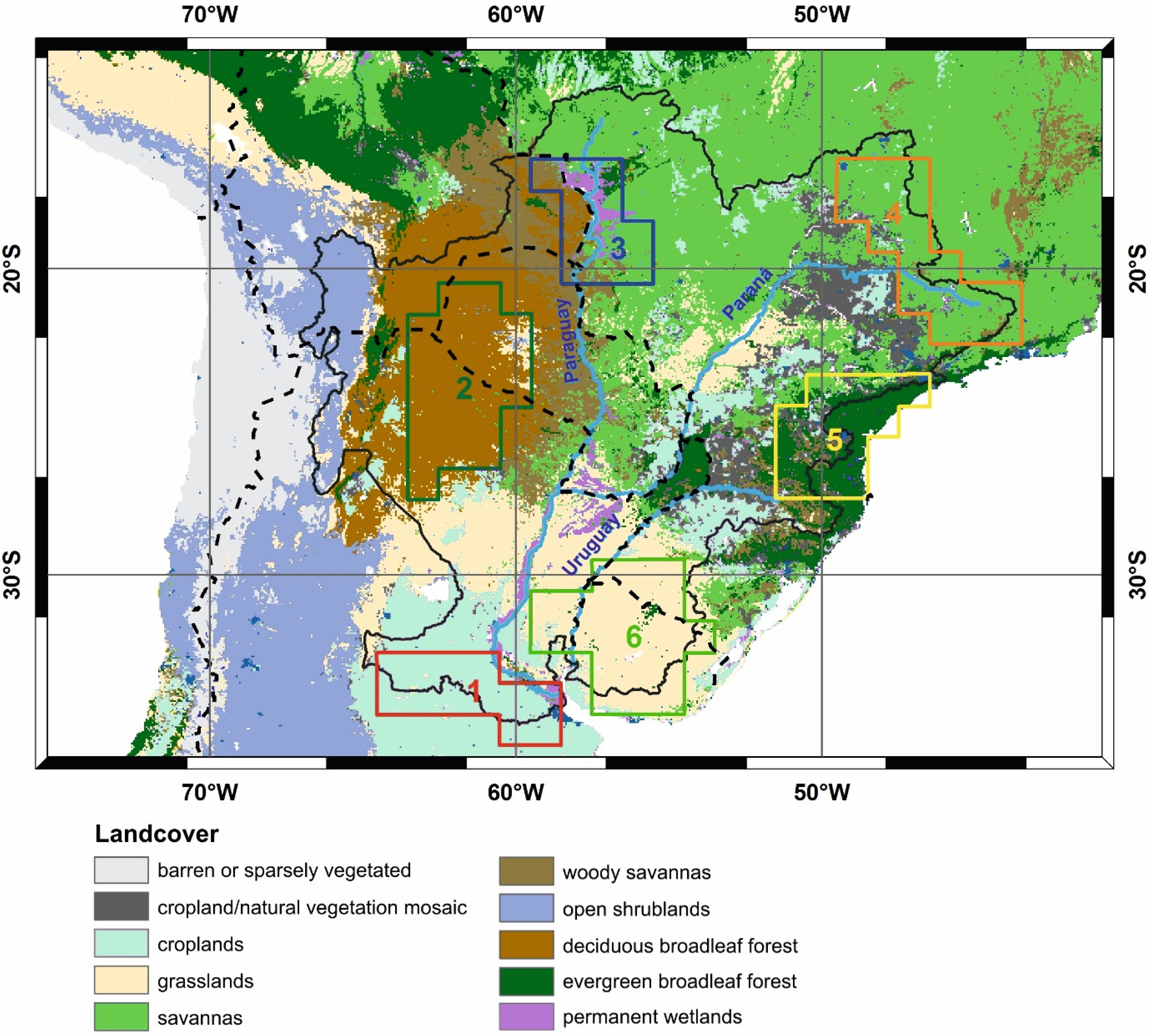
  • Southern cropland (Pampas; Figure 1, sub-region 1) and southern grassland (Campos; Figure 1, sub-region 6): The Pampas and the Campos are two major sub-regions of the major South American grassland, which stretches from the south of Brazil to Argentina, comprising more than 700,000 km2. The climate changes from west to east from humid to dry-subhumid [32]. The plain contains the most fertile soils of the La Plata Basin. The Campos has continental climate with frequent frost in winter and daily maximum temperature above 36 °C in summer. Rainfall is distributed throughout the year but changes strongly between years [33]. The annual mean precipitation in the North (1600 mm) is larger than in the South (1200 mm). The Campos is mainly used for grassland-based livestock production [34]. This is different for the Pampas. This region is intensively used by agriculture. The climate is similar to the Chaco with the main precipitation falling from October to March.
  • Western deciduous broadleaf forest (Chaco; Figure 1, sub-region 2): The Chaco is a subtropical area and located west of the Paraguay River and east of the Andes [35]. It is the warmest region in the La Plata Basin. In summer, the daily maximum temperature often exceeds 45°. The rainy season usually takes place between September and April. The semi-arid plains of the Chaco are dominated by dry woodland, which (approaching to the east) transform into more open savannas (Figure 1).
  • Wetland Pantanal (Figure 1, sub-region 3): The Pantanal is one of the world’s largest wetlands with enormous biodiversity, covering about 100,000 km2 of the Paraguay Basin [36]. It behaves as a regulator for the entire La Plata Basin, by slowing the streamflow of the Paraguay River before its junction with the Paraná River [29]. Annual totals of precipitation exceed 1300 mm. In December, the precipitation maximum takes place, reaching about 200 mm. In July and August, the precipitation is close to zero [37].
  • Northern savanna (Cerrado; Figure 1, sub-region 4): The Cerrado is a rather moist savanna region with an average annual precipitation of around 1500 mm. The climate is seasonal with a very strong dry period, spanning from April to September. The temperatures are mild, ranging from 22° to 27°. Large parts of the Cerrado have been transformed into pasture or are used for cash cropping [38].
  • Eastern evergreen broadleaf forest (Mata Atlantica; Figure 1, sub-region 5): Originally the Atlantic forest was one of the world’s largest rainforests, covering approximately 150 million ha. Nowadays, only smaller fragments exist due to intensive deforestation and agricultural use [39]. The region has the highest average annual precipitation (above 2000 mm) in the La Plata Basin [30] and receives precipitation during the whole year. The climate is tropical to subtropical. The month of maximum precipitation varies from north (boreal summer) to south (boreal winter). Therefore, the annual cycle of precipitation for the whole region shows three peaks [40]: one at the beginning of spring, one in the middle of summer, and one in winter (with respect to boreal seasons). Due to the height of the region, frost occurs frequently during winter and precipitation may fall in some sub-region as snow (e.g., high places of Santa Cantarina State).

3. Data

Table 1 gives an overview of the different data products used in this study and highlights differences in spatial resolution, units, and representation. For the analysis, all data sets were processed for the overlapping time span (September 2007–August 2011) with a temporal resolution of one month and a spatial resolution of 1°. If soil moisture or precipitation data sets were compared with GRACE, a harmonization procedure was applied (see Section 4.2).
Table 1. Specifications of the main data sets of soil moisture and total water storage.
Satellite GravimetryRemote SensingHydrological Model
SourceGRACEASCATAMSR-EWGHM
ProductLevel 2, RL05, German Research Centre for Geosciences (GFZ)Level 2 Soil Moisture at 25 km Swath Grid
EUMETSAT, Vienna University of Technology (TU Wien)
LPRM/AMSR-E/Aqua Daily L3 Surface Soil Moisture, Vrije Universiteit Amsterdam, and NASA GSFCVersion 2.2, German Research Centre for Geosciences (GFZ), University of Frankfurt
Reference[41][42][43][44]
Parameterchange in total water storagesurface soil moisturesurface soil moistureroot zone soil moisture, precipitation
Availability2002–present2007–present2002–20111901–present
Temporal Resolutionmonthlydailydailymonthly
Spatial Resolution300 km25 km25 km0.5°
Coverageglobalglobalglobalglobal
Unitmm% (0% dry, 100% wet)m3/ m3mm
RepresentationSpherical harmonic coefficientsAscending and descending tracks0.25° world map with descending tracks0.5° world map

3.1. Satellite Soil Moisture

For this study, two satellite soil moisture data sets with a large overlap in mission operation were selected. The first data set of the active microwave scatterometer ASCAT is provided by EUMETSAT and contains additional information on quality control. We apply the same thresholds as proposed by [17], excluding data points with topographic complexity, inundation and wetland fractions greater than or equal to 50%, and soil moisture error greater than or equal to 10%. Aiming at a better understanding of data quality and a large spatial coverage, these criteria are less stringent as those used in data assimilation studies.
The second data set was developed by Vrije Universiteit Amsterdam and NASA’s Goddard Space Flight Center and originates from the passive microwave sensor AMSR-E. As in many other studies [45,46,47], only descending tracks were used herein. For quality control, data points were excluded if any of the flags (which are delivered with the data set) indicating high vegetation in the X-band, high vegetation in the C-band, or frozen ground were set.
ASCAT and AMSR-E, which operate in the C-band at 5.3 and 6.8 GHz, respectively, provide information for the uppermost portion (<5 cm) of the top soil layer. ASCAT data are provided as percentages of dryness, where 0% corresponds to the driest soil surface conditions (lowest backscatter coefficients) and 100% corresponds to wettest soil surface conditions (highest backscatter coefficients). AMSR-E data give information on the volumetric soil moisture content [m3H2O/m3soil].

3.2. WaterGAP Global Hydrology Model (WGHM)

The global hydrology and water use model WaterGAP has been developed for the assessment of global water resources and water balances of large river basins [48]. In addition to water use models for different sectors, WaterGAP comprises the Global Hydrology Model (WGHM), which calculates daily water storage and water flow for all continental areas except Antarctica with a spatial resolution of 0.5°. WGHM accounts for all main continental water storage components including groundwater, soil moisture, snow, canopy storage, and surface waters in lakes, rivers, wetlands, and reservoirs. The water mass of all components adds up to the total continental water storage, which was analyzed by [49] and compared to TWS measurements from GRACE in various studies (e.g., [50,51,52,53]). In this study, the latest version of WGHM in WaterGAP2.2 was applied [44]. For model calibration against observed river discharge time series, 1319 gauging stations worldwide are used in WGHM. The precipitation data set used as model input in this study was the Monitoring Product Version 4.0 taken from the Global Precipitation Climatology Center (GPCC) [54]. Other climate forcing data such as temperature, cloudiness, and number of rainy days per month were taken from operational forecast or analysis data of the European Centre for Medium-Range Weather Forecasts (ECMWF). Soil moisture in WGHM is calculated for one soil layer of which the thickness varies with the land cover depending on the vegetation rooting depth. The maximum available soil water capacity is calculated by multiplying the rooting depth by the total available water capacity in the uppermost meter of the soil [48].

3.3. GRACE

In this study, we used GRACE RL05 Level-2 data provided by the GFZ German Research Centre for Geosciences [41]. Original GRACE observations of the time-variable gravity include the effects of all mass changes in the atmosphere, on the Earth’s surface, and in its interior. During pre-processing, the gravity signal is reduced for mass changes within the atmosphere and the ocean as well as for solid Earth tides [41]. The remaining signal predominantly provides information on changes in continental water storage. However, for some regions, post-glacial rebound [55] or other non-hydrological signals may need to be considered [56,57]. It is assumed that in the La Plata Basin, the GRACE signal mainly maps changes in soil moisture, surface water, and groundwater storage.
GRACE data are usually provided in spherical harmonic coefficients with a temporal resolution of one month. In this study, spherical harmonic coefficients were processed up to degree and order 70, corresponding to a spatial scale of approximately 300 km. GRACE data show longitudinal stripes due to correlations among certain spherical harmonic coefficients [58]. Further errors result from the orbit configuration of the twin satellites [59] and sub-monthly mass changes that are not captured by the background models in the course of the abovementioned reduction process (i.e., aliasing of high-frequency mass variations) [60]. To remove correlated errors in the coefficients, the spherical harmonics of the GRACE data were filtered with a least-squares polynomial filter [58]. Furthermore, an isotropic Gauss filter [59] with 300-km half-wavelength radius was applied. Subsequently, the spherical harmonic coefficients were converted back into geographical grids of 1° × 1°.
The main remaining errors in the GRACE data arise from spatial leakage and signal loss, as the filtering attenuates both the noise and parts of the signal and enhances leakage of mass variations from the surrounding regions into the study area. In this study, we assume that all data sets are similarly affected by spatial leakage due to identical processing (see Section 4.2).

3.4. El Niño/La Niña Index

The Climate Prediction Center of the United States National Oceanic and Atmospheric Administration (NOAA) provides the Oceanic Niño Index (ONI) to identify El Niño and La Niña events in the tropical Pacific [61]. The ONI is calculated from the three-month mean sea surface temperature anomaly for the Niño 3.4 region (5°N–5°S, 120°–170°W). If five consecutive overlapping three-month periods exceed a certain threshold, they are classified as El Niño (warm, positive anomaly) or La Niña (cool, negative anomaly) events [62]. The threshold is set to 1.5 for strong events, 1.0–1.4 for moderate events, and 0.5–0.9 for weak events [63].

3.5. EM-DAT, the International Disaster Database

EM-DAT (the OFDA/CRED International Disaster Database—www.emdat.be—Université catholique de Louvain, Brussels, Belgium) is a global database on natural and technological disasters, and it is maintained by the Centre for Research on the Epidemiology of Disasters (CRED). From 1900 onward, more than 17,000 disasters that meet at least one of the following criteria have been registered [64]:
-
ten or more people killed;
-
one hundred or more people affected;
-
declaration of a state of emergency; and
-
call for international assistance.
Figure 2. Location of natural disasters in the La Plata Basin from October 2007 to July 2011 based on the International Disaster Database EM-DAT.
Remotesensing 07 07324 g002
The main EM-DAT disaster types considered in this study were hydrometeorological in nature and classified as storms, floods, extreme temperature, and droughts. We neglected wet mass movements, landslides, avalanches, and land subsidence as their impacts are limited to local scales. We also neglected wildfires. A further criterion for the selection of events was the size of the affected area (events were not considered, e.g., if only one city was affected). Figure 2 shows a rough spatial distribution of the selected disasters within the La Plata Basin. Most of the disasters were registered in densely populated regions such as the east coast of South Brazil and the surroundings of the metropolitan area Gran Asunción in Paraguay [65]. In sparsely populated regions such as the Chaco, the Pantanal, and the Campos, only a few events were listed. This is due to the fact that extreme weather events are only classified as natural disasters within EM-DAT if they had a high impact on society.

4. Methods

4.1. Scaling

ASCAT and AMSR-E only map the near-surface soil moisture, whereas WGHM provides the soil moisture content for the entire root zone. All three data sets cannot be compared directly in terms of magnitude. Additionally, ASCAT data are provided as percentages of dryness. To harmonize the units and approximate the root zone soil moisture for all data sets, we scaled ASCAT and AMSR-E data with respect to the soil moisture content provided by WGHM. A pixel-wise scaling algorithm was applied because the depth of the soil column may vary among the pixels. The time series of each pixel was scaled with respect to the minimum and maximum soil moisture values of the same pixel, as provided in the reference soil moisture data (WGHM herein).
The simple scaling has the advantage that it does not influence the correlation between data sets, as shown by [47]. For example, the correlation between scaled ASCAT soil moisture and GRACE TWS yields the same correlation coefficients as the correlation between unscaled ASCAT soil moisture and GRACE TWS. However, the simple scaling has the disadvantage that it does not account for the heterogeneous vertical distribution of soil moisture. Also the maximum and minimum values of root zone soil moisture, taken from the WGHM for the scaling, may contain errors. Due to this limitation, soil moisture values are not discussed in absolute terms in this study.
Alternative algorithms exist, which derive root zone soil moisture from satellite surface soil moisture. For example, several studies suggest the use of an exponential filter to calculate the so called soil water index (SWI) [66,67]. The algorithm comprises a parameter (called time characteristic length), which depends on the depth of the root zone and the soil properties. Such an algorithm is not used here, as it requires reference data (which is optimally in situ data) for calibration. Furthermore, in the case of filtered data, correlation results are not any more independent from the reference data. For example, the correlation between the SWI from ASCAT and GRACE TWS does not yield the same correlation coefficients as the correlation between unscaled ASCAT soil moisture and GRACE TWS.

4.2. Harmonization

The data sets from satellite gravimetry, soil moisture remote sensing, and hydrological models differ in temporal and spatial resolution, representation (grid format vs. spherical harmonics), and processing (e.g., filtering). To avoid these differences that strongly impact the analysis, all data sets were harmonized in a first step, as thoroughly described in [17]. Due to the particular processing of GRACE data (see Section 3.3), all soil moisture data sets were converted into spherical harmonics of degree and order 70 and an isotropic Gauss filter with a 300-km half-wavelength radius was applied. Subsequently, the spherical harmonic coefficients were converted back into geographical grids of 1° × 1°. Regions affected by snow, ice, and post-glacial rebound or very low variation in soil moisture must be masked out when comparing soil moisture data with GRACE [17]. In the case of the La Plata Basin, no masking is necessary.
The main impact of the harmonization procedure is the spatial smoothing of the data, which causes damping of the signal, loss of detail, and reduction of noise. This leads to an increase in the correlation coefficients between the data sets. Therefore, data are harmonized in this study only if a comparison with GRACE data is sought (e.g., comparing GRACE with satellite soil moisture products). Otherwise (e.g., for the comparison of different remote sensing soil moisture products), only the spatial resolution is harmonized by computing the simple average of all data points falling into a 1° × 1° grid cell. In any case, the temporal resolution of all data sets is aggregated monthly, which is similar to the standard GRACE resolution.

4.3. Correlation and Principal Component Analysis

Two well-known methods were used for the comparison of data sets. The first one is the Pearson product-moment correlation coefficient [68], which is defined as the covariance of two variables divided by the product of their standard deviations. As in other studies, which focus on the correlation of various soil moisture data sets [69,70,71], Fisher’s z-transformation is used to calculate confidence limits for the Pearson product-moment coefficients.
The second method is the principal component analysis (PCA). With the help of PCA, a spatio-temporal signal (e.g., a time series of maps) is split into a series of empirical orthogonal functions (EOFs) that describe the spatial base pattern of the signal. The corresponding coefficients are called principle components (PCs) and describe the temporal behavior of the signal. The first mode (first pair of EOF and PC in the series) describes the most dominant part of the signal. Higher modes have decreasing importance [72]. PCA has already been used in arid environments to compare satellite soil moisture products and GRACE [73].

4.4. Sample Cross-Covariance Function

To identify possible time shifts in the signals of different data pairs, the time lag maximizing the cross correlation between two signals was calculated. Therefore, the sample cross-covariance function described by [74] was used. It provides an estimate of the covariance (c) between two time series xt ([x1,x2,… xT]) and yt ([y1,y2,… yT]) for a defined time lag k:
c x y ( k ) = { 1 T t = 1 T k ( x t x ¯ ) ( y t + k y ¯ )   k = 0 , 1 , 2 , n 1 T t = 1 T + k ( y t y ¯ ) ( x t + k x ¯ )   k = 0 , 1 , 2 , n
where x ¯ is the mean of the first time series and y ¯ is the mean of the second time series. The formula for estimating the cross correlation (r) is:
r x y ( k ) = c x y ( k ) s x s y   k = 0 , ± 1 , ± 2 , ± n
where sx is the variance of the time series xt ( c x x ( 0 ) ) and sy is the variance of the time series yt ( c y y ( 0 )   ). In this study, xt is the signal of one data set, yt is the signal of another data set, T = 48 months, and n = 6 months.
Figure 3. Monthly mean (column 1) and monthly anomaly (column 2) for soil moisture from ASCAT, AMSR-E and WGHM (ASCAT and AMSR-E are scaled with respect to WGHM), and for precipitation from GPCC for the entire La Plata Basin (row 1) and the different sub-regions delineated in Figure 1 [including the northern savanna (row 2), the wetland Pantanal (row 3), the western deciduous forest (row 4), the eastern evergreen broadleaf forest (row 5), the southern grassland (row 6), and the southern cropland (row 7)].
Remotesensing 07 07324 g003

5. Results and Discussion

5.1. Comparison of Soil Moisture Data Sets

Before linking the signatures of soil moisture to extreme weather conditions, the different global soil moisture data sets of the hydrological model WGHM and the two satellite products ASCAT and AMSR-E were compared. Figure 3 and Figure 4 show that ASCAT and WGHM agree well in most parts of the La Plata Basin with correlation coefficients above 0.7 for the monthly time series (90% confidence interval ranges from 0.6 to 1). Exclusively in the evergreen broadleaf forest in the eastern part of the study area, the soil moisture signal from WGHM lags several months behind the ASCAT signal (lag −3–−6) and therefore has to be shifted forward in time (Figure 4, row 2, column 3). However, even if the time shift is implemented, the correlation does not improve much (Figure 4, row 3, column 3). For soil moisture from AMSR-E and WGHM, the correlation coefficients are lower than those for ASCAT and WGHM. Especially in the western part of the basin, they are negative or close to zero since the seasonal signals are out of phase (Figure 3, column 1, rows 3–4 and Figure 4, row 1, column 2). The poor correlation values agree with the results of [51], which reports large errors for the AMSR-E signal in the La Plata Basin.
Figure 4. Correlation (row 1), time shift in months (row 2; negative values indicate that the seasonality of the first soil moisture product lags behind the second product), and correlation after the implementation of time shift (row 3) for soil moisture from AMSRE and ASCAT (column 1), AMSRE and WGHM (column 2), and ASCAT and WGHM (column 3).
Remotesensing 07 07324 g004
In the eastern evergreen broadleaf forest, neither ASCAT nor AMSR-E agree well with soil moisture from WGHM. Although WGHM model deficits cannot be excluded, this indicates that in this region, the microwave signal received by ASCAT and AMSR-E is severely degraded by the topographic complexity [69] and/or the very high foliage density, which shield the soil moisture signal [75].
Figure 3 shows that in the southeastern part of the basin (rows 6 and 7), the seasonal pattern of precipitation and soil moisture for the relatively short study period considered here is dominated by the anomaly of the El Niño event in the boreal winter of 2009/2010. The absence of a marked seasonality in this region in the absence of extreme events is also described by [30] for streamflow data. The strong anomaly in the Campos region (column 2, row 6) is consistent with a severe flood that Uruguay suffered from in November 2009, affecting 22,000 people. In the eastern evergreen broadleaf forest (column 2, row 5) the anomaly has approximately the same amplitude as the seasonal signal and shows high fluctuation. This region, including the state of São Paulo, Brazil, is densely populated [65]. Both facts explain why the region was struck by five major disasters within only four years (compare Figure 2).

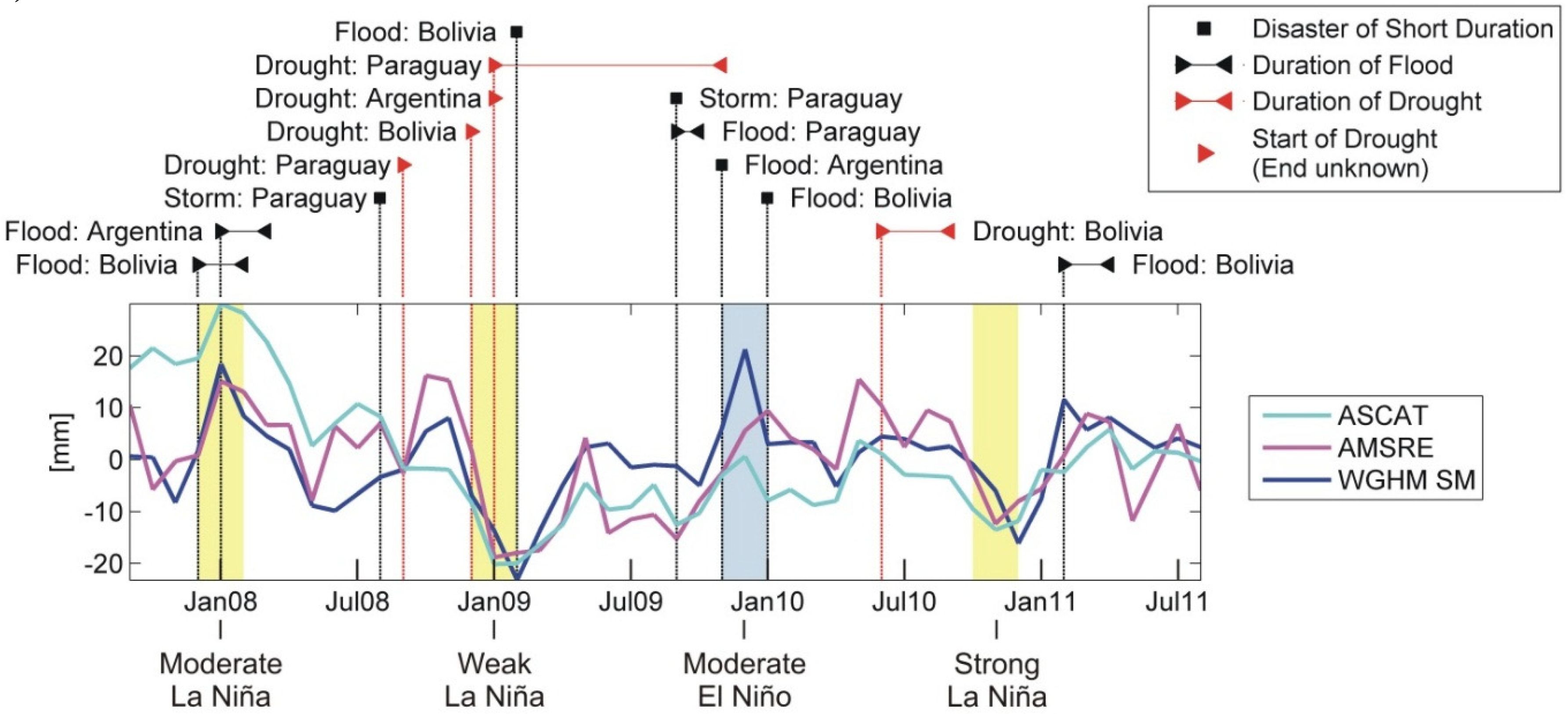
5.2. Hydrological Extremes

The comparison of the anomalies of different hydrological parameters in the La Plata Basin (Figure 5) shows the close connection between soil moisture and precipitation. Furthermore, the anomalies are in agreement with time variations of water levels at different locations in the La Plata Basin, as presented by [23]. The comparatively smooth GRACE time series is an expression of the integrative nature of TWS that, to some extent, balances out short-time variations in individual storage components. Furthermore, anomalies of GRACE TWS tend to be shifted by a few months with respect to soil moisture and precipitation, as it takes time until precipitation extremes accumulate within surface and ground water storage. A drastic decrease in soil moisture can therefore be an indicator for an upcoming deficit or surplus in total water storage. One example is the La Plata drought in 2009, wherein soil moisture was lowest between December 2008 and January 2009, and total water storage reached its minimum in May 2009. The minimum soil moisture in December 2008 agrees with the fact that the drought was declared and registered in January 2009 as a natural disaster within the International Disaster Database EM-DAT. Furthermore, the local minima for soil moisture in May 2009 and the decrease in total water storage until May 2009 illustrate that the drought lasted for several months until approximately November, 2009. The clear signal of the La Plata drought of 2008/2009 in GRACE TWS was also observed by [20]. The flood period in the boreal winter of 2009/2010 (as supported by [22]) and the flood period in the beginning of 2011 are also visible in the GRACE data. Apart from these events, it was not possible to link anomalies of GRACE TWS directly to the listed natural disasters. This is due to the coarse spatial resolution of the GRACE sensor and its low sensitivity to small mass changes. Also short-time events such as storms might not affect all water storage components contained in TWS.
In contrast, almost all droughts and floods could be identified as single events or as accumulated events (e.g., winter 2009/2010 and March and April 2011) in at least one of the soil moisture data sets from ASCAT, AMSR-E, or WGHM. The only exception is the flood in Brazil in November 2010, which affected the northeastern fringe area of the basin, including parts of Minas Gerais, São Paulo, and Rio de Janeiro.
Figure 5. Disasters as registered by the International Disaster Database EM-DAT for the La Plata Basin (top), number of people affected and killed for each disaster (second from top), monthly anomalies as basin averages after data harmonization for TWS from GRACE, precipitation from GPCC (third from top), and soil moisture from ASCAT, AMSR-E, and WGHM (ASCAT and AMSR-E are scaled with respect to WGHM; fourth from top), and El Niño and La Niña anomalies as described by NOAA through the Oceanic Niño Index (ONI; bottom).
Remotesensing 07 07324 g005
Furthermore, some meteorological events (storms and cyclones) could be linked to anomalies in the soil moisture data, e.g., the storm in Paraguay in August 2008. During this month, precipitation data from GPCC and the two soil moisture data sets from AMSR-E and ASCAT show local maxima.
Figure 6 emphasizes that specific extreme events can be identified more clearly when focusing on smaller regions. For example, the flood in Bolivia from December 2007 to February 2008 is clearly visible in all soil moisture signatures when averaging over the western sub-region in the Chaco only. At the same time, it became clear that the minima of the AMSR-E signal in June 2010, as seen in the basin average in Figure 5, is not associated with the drought in Bolivia. Thus, a differentiation into hydrological extreme events of basin-wide character or of regional extent is only possible with the given data sets.
Figure 5 does not show the expected below average precipitation in the La Plata Basin during the moderate La Niña period of 2007/2008. However, atypical precipitation patterns during this La Niña period were also observed in southeastern Australia [76]. From the summer of 2008 onward, there is a strong relationship between variations in soil moisture and the ONI (Figure 5). The first phase of the La Plata drought in 2009 fell into the weak La Niña period during the boreal winter of 2008/2009, which is also supported by [20]. Furthermore, the moderate El Niño period in the boreal winter of 2009/2008 coincides with the very high soil moisture values in December 2009 and several floods affecting Argentina, Brazil, Bolivia, and Uruguay. The anomaly is also visible in TWS from GRACE and initiated by high precipitation during November and December 2009. The strong La Niña period during the boreal winter of 2010/2011 is shown as local minima during November 2010 for all parameters (except for AMSR-E).
Figure 6. Disasters as registered by the International Disaster Database EM-DAT for the deciduous broadleaf forest (Chaco) in the western part of the La Plata Basin (see Figure 1) (top) and monthly anomalies of soil moisture from ASCAT, AMSR-E, and WGHM (ASCAT and AMSR-E are scaled with respect to WGHM; bottom).
Remotesensing 07 07324 g006
The dominant spatial patterns of the various data sets and the major differences among them were further analyzed by PCA. The first, second, and third modes explain approximately 60%, 25%, and 5% of the TWS signal from GRACE and the soil moisture signals from ASCAT and WGHM, respectively. For AMSR-E, the first three modes account for 50%, 25%, and 10% of the signal. The first mode mainly represents the seasonal part of the signal (Figure 7, row 1). In the PCs, no time shift between the seasonal cycles of the different soil moisture products is visible. For GRACE, the phase of the seasonal signal is approximately two months later. The EOFs of the first mode show a characteristic opposing pattern in the northern part of the La Plata Basin versus in the southeastern part (Figure 8, row 1). The inverse annual signal for AMSR-E visible in Figure 3 (column 1, rows 3–4) in the western and northern parts of the basin is reflected by the inverse signs of the EOFs of AMSR-E compared with the EOFs of the other soil moisture products in this region. The nonconformity between AMSR-E and other soil moisture data sets is also reflected in the PCs and EOFs of the second mode.
Figure 7. Principal components for the first, second, and third modes for soil moisture from AMSR-E, ASCAT, WGHM (AMSR-E and ASCAT data are scaled with respect to WGHM), and GRACE after data harmonization. For the second and third modes, the shaded areas indicate the La Plata drought in 2009 (yellow) and the flood period associated with El Niño in the boreal winter of 2009/2010 (blue).
Remotesensing 07 07324 g007
Figure 8. Empirical orthonormal functions for the first, second, and third modes for soil moisture from AMSR-E (column 1), ASCAT (column 2), and WGHM (column 3) (AMSR-E and ASCAT data are scaled with respect to WGHM) and total water storage from GRACE (column 4) after data harmonization.
Remotesensing 07 07324 g008
The PCs of the second and third modes show secondary minima for soil moisture from ASCAT and WGHM during the La Plata drought in 2009 (Figure 7, rows 2–3). This indicates that the southern, central (Figure 8, row 2, columns 2–3), and eastern parts (Figure 8, row 3, columns 2–3) of the basin were mostly affected. The described spatial pattern is in agreement with precipitation maps for the La Plata Basin in winter and spring 2009 from the Argentinean National Meteorological Service (SMN), as presented by [22].
Similarly, the flood period associated with El Niño in the boreal winter of 2009/2010 can be identified in the PCs of the third and second modes of the soil moisture data. As the anomaly in the third mode (Figure 7, row 3) appears before the anomaly in the second mode (Figure 7, row 2), the eastern part of the basin (Figure 8, row 3, columns 2–3) followed by the southeastern part (Figure 8, row 2, columns 2–3) were affected. This sequence of spatial patterns is also supported by the precipitation anomalies of SMN [22]. Furthermore they are reflected in the signatures of precipitation and soil moisture in Figure 3 (column 2, rows 5–7).
For GRACE, the two periods of extremes are also clearly visible in the PCs of the second and third modes. For the La Plata drought in 2009, the second mode is shifted by a few months and the third mode by several months with respect to the signatures of soil moisture. The EOF of the second mode (Figure 8, row 2, column 4) shows that the northeastern and central parts of the basin were first affected. Then, based on the EOF of the third mode (Figure 8, row 3, column 4), the southern part was affected. The temporal development of the drought provided by the PCs is similar to the results of [17]; the minimum values of water storage in the entire basin occurred during the first half of 2009 followed by strong but regionally confined low water storage in the southern part in July and August.
For the first half of 2009, the soil moisture data show that the largest anomalies were in the southern, central and eastern parts of the basin. However, within the International Disaster Database EM-DAT, the largest impact of the drought was registered in the central and northwestern parts of the basin, affecting more than 227,000 people in Bolivia and Paraguay. It is possible that the International Disaster Database EM-DAT lacks information on the impact of the drought; for example, the database does not contain any information on the drought situation in Uruguay. A situation report of the United Nations Development Program in Uruguay (dated at the beginning of the drought in January 2009) clarifies that Uruguay was affected by the drought (e.g., through food shortages and lack of water for livestock) [77]. However, the report also states that there was a lack of integral information on the impact of the drought and the economic consequences. This example shows that databases like EM-DAT might be incomplete due to the difficulty in collecting and receiving quantitative data on an international level. Moreover, it should be noted that the disaster classification given by EM-DAT explicitly considers the vulnerability of the region, which is defined by demographic factors such as population density (which is relatively low in Uruguay [65]), environmental factors (e.g., state of resource degradation and depletion), social factors (e.g., traditional knowledge systems), and economic factors (e.g., economic status of individuals, communities, and nations) [78]. In contrast, the soil moisture and TWS products only reflect the physical factors in terms of a subset of hydrometeorological hazards.

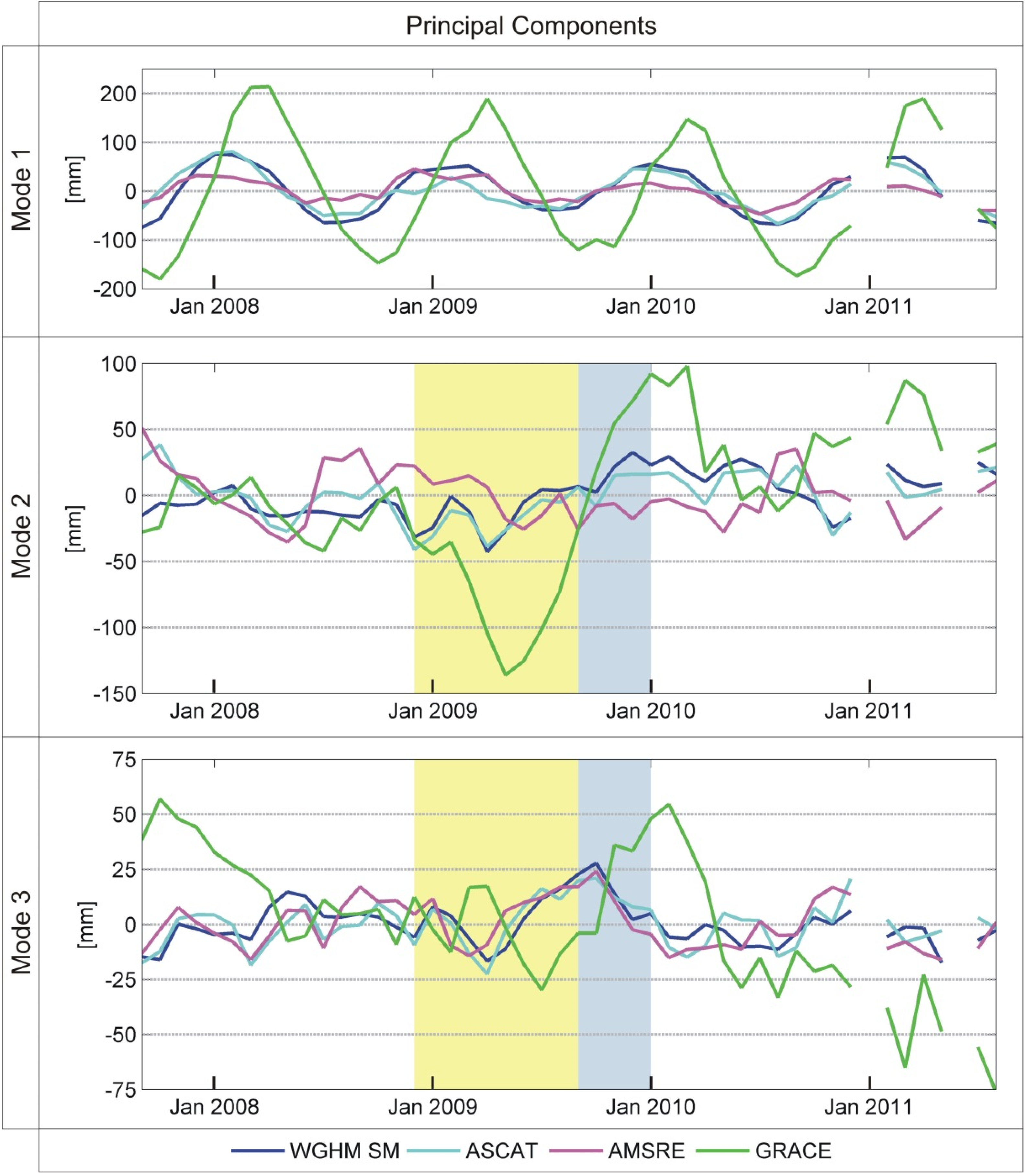
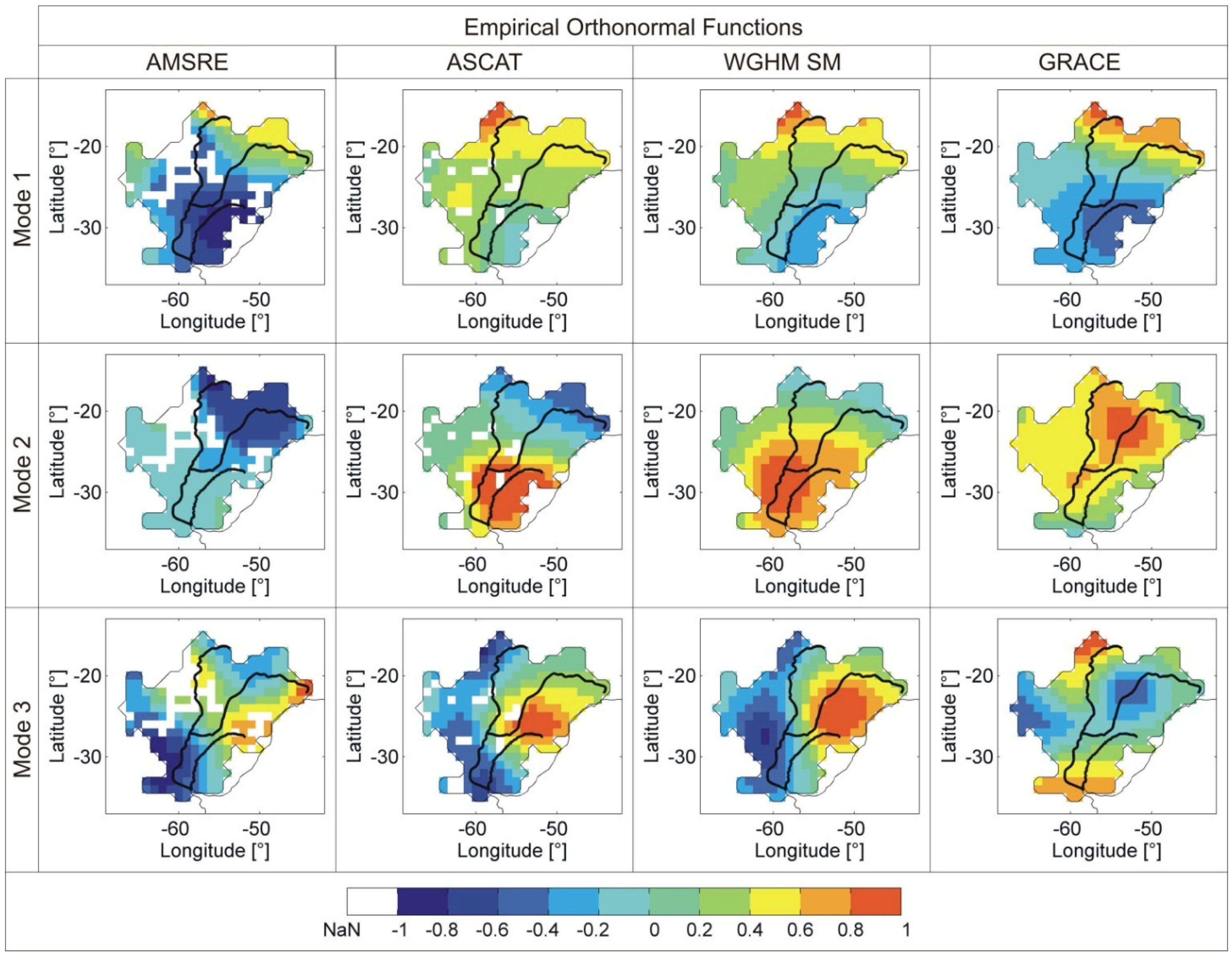
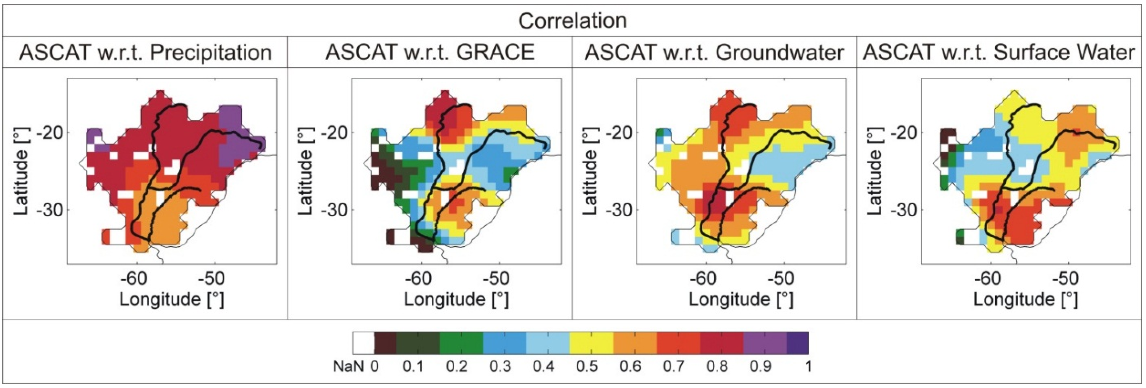
5.3. Soil Moisture and GRACE TWS

Figure 9 highlights two regions where the dynamics of soil moisture from ASCAT and TWS from GRACE are interrelated. In both regions, soil moisture is not the dominant component of TWS, but it is closely linked to the most dominant water storage components (surface water and groundwater herein). The first region with high agreement is the northern wetland Pantanal (correlation coefficients are around 0.8, 90% confidence interval ranges from 0.7 to 0.9). In the Pantanal, the shallow groundwater table may rise and saturate the surface soil or fall and leave the surface soil dry [79]. Therefore, near-surface soil moisture dynamics monitored by ASCAT can be expected to be a good indicator of TWS variations. The second region with a good correlation between ASCAT and GRACE (correlation coefficients range from 0.6 to 0.7; 90% confidence interval is 0.5 to 0.8) ranges from the junction of the Paraguay and Paraná Rivers, which is surrounded by wetlands (Figure 1), to the southeastern coast of the basin. Again, in the wetland region, the dynamics of groundwater and soil moisture tend to be closely linked. Approaching the coast, the connection to surface water is stronger.
The correlation of ASCAT time series to precipitation is high for most parts of the study area (correlation coefficients are above 0.7 as shown in Figure 9 and the 90% confidence interval ranges from 0.6 to 0.9). This is reasonable as near-surface soil moisture variations seen by ASCAT are directly triggered by the precipitation dynamics. Nevertheless, the correlation tends to decrease toward the southeastern downstream parts of the basin, whereas the correlation of ASCAT with WGHM simulation-based surface water storage simultaneously increases. In this region the groundwater recharge is high (>100 mm) [23]. This implies that the relevance of local rainfall-induced soil moisture variations decreases in favor of soil moisture variations caused by allochthonous processes at the regional scale, i.e., surface water inflow from upstream areas of the river basin.
Figure 9. Correlation after data harmonization for soil moisture from ASCAT with respect to precipitation from GPCC (column 1), total water storage from GRACE (column 2), groundwater from WGHM (column 3), and surface water storage from WGHM (column 4).
Remotesensing 07 07324 g009

6. Conclusions

In this paper, we investigated how total water storage from GRACE and soil moisture from two remote sensing satellites sensors (ASCAT and AMSR-E) and one hydrological model (WGHM) map extreme weather events in the La Plata Basin of South America. Information from the International Disaster Database EM-DAT was included in the analysis to place special emphasis on extreme hydrometeorological events that were highly destructive. Furthermore, the link between variations in soil moisture and TWS was analyzed. Therefore, the distinct representations and formats of all data sets were harmonized by conversion in spherical harmonics and filtering whenever any data set was compared with GRACE. For comparison, we correlated different data pairs, analyzed the time shift between seasonal cycles, and performed PCA to split the signal in spatial base functions and temporal components.
First, the different soil moisture data sets were compared. The results indicate that soil moisture products from ASCAT and WGHM are strongly correlated (correlation coefficients above 0.7) in the majority of the sub-regions of the La Plata Basin. For AMSR-E, the correlation coefficients take values above 0.6. However, in the eastern deciduous broadleaf forest, the western evergreen broadleaf forest, and the wetland Pantanal, signatures of AMSR-E differ strongly from those of both WGHM and ASCAT. In the eastern forested region, neither ASCAT nor AMSR-E correlate well with soil moisture from WGHM, possibly due to signal disturbance by the topographic complexity and dense vegetation in this region.
Second, extreme meteorological and hydrological conditions, specifically those that have been classified as natural disasters within the International Disaster Database EM-DAT, were brought into focus. Thus, two independent data sources were linked. On the one hand, signatures of hydrological variables were analyzed to gather information on hydrometeorological extremes. On the other hand, natural disasters that affected the La Plata Basin during the analyzed time period were identified to include information on the number of people affected or killed by extreme events. The analysis of both data sets showed that most of the strong variations in soil moisture match temporally with natural disasters (droughts, floods, or storms). For two hydrologic extreme periods that led to several natural disasters (the La Plata drought in 2009 and the flood period in the winter of 2009/2010), it could be observed that soil moisture first changes drastically followed by TWS from GRACE with a delay of a few months. In these two cases, soil moisture serves as an indicator for the later deficit or surplus in TWS.
Out of four El Niño and La Niña events during the analyzed time period, three events match with extreme soil moisture and TWS conditions. These events include the weak La Niña event in 2008/2009, the moderate El Niño event in 2009/2010, and the strong La Niña event in 2010/2011. The most meteorologically and hydrologically affected areas were the southern, central, and eastern parts of the La Plata Basin. However, based on the International Disaster Database, the main impacts were registered in the central and northwestern parts of the basin. This reveals that several limitations have to be considered when linking extremes in soil moisture or total water storage to natural disasters. On the one hand, not all extreme hydrologic events have large impacts on society. This might be due to the fact that the destructiveness of a disaster not only depends on the magnitude of the hydrometeorological extreme indicated by GRACE, ASCAT or AMSRE but also on the vulnerability of the region considered in EM-DAT, which largely depends on other factors such as the preparedness of the population and the population density. On the other hand, the collection of quantitative information on the impacts of disasters is challenging on an international level. Therefore, limited data availability in the EM-DAT database for the southern parts of the study area cannot be excluded.
Analyzing the hydrological signals as basin averages and with a temporal resolution of only one month makes the identification of regional or short-term events difficult. Nevertheless, it could be shown that the remote sensing products used here allow for differentiating hydrological extreme events of basin-wide character or of local to regional extents.
Finally, the discussion focused on possible interdependencies between the dynamics in soil moisture and the dynamics in TWS. A close link between soil moisture and total water storage was identified in regions where groundwater or inflow of surface water from upstream areas influences the dynamics of soil moisture.

Acknowledgments

We thank the International Graduate School of Science and Engineering of Technische Universität München (TUM) for funding this research through the project “Signals of Climate Variability in Continental Hydrology from Multi-Sensor Space and In-situ Observations and Hydrological Modeling” (CLIVAR-Hydro). We are also thankful to the Department of Geophysics at Universidad de Concepcion for supporting Sarah Abelen during her research stay in Chile. Andreas Güntner received funding for this study from the European Union’s Horizon 2020 research and innovation programme under grant agreement No 637010 (EGSIEM).
Furthermore, we thank Professor Wolfgang Wagner for his helpful comments and advice with respect to the interpretation of the satellite-based soil moisture data sets. This work was supported by the German Research Foundation (DFG) and the Technische Universität München within the funding programme Open Access Publishing. The MODIS land cover product used here is courtesy of the online Data Pool at the NASA Land Processes Distributed Active Archive Center (LP DAAC), USGS/Earth Resources Observation and Science (EROS) Center, Sioux Falls, South Dakota.

Author Contributions

As part of her doctoral thesis, Sarah Abelen was mainly responsible for the remote sensing soil moisture data sets, the data harmonization and the implementation of the methodological parts, including the correlation analysis, PCA, and the Sample Cross Covariance Function. Furthermore, she integrated information from the EM-DAT International Disaster Database into the analysis. Florian Seitz is the principal investigator of IGSSE’s project CLIVAR-Hydro. He contributed to the paper through the pre-processing of monthly GRACE L2 gravity field data. Rodrigo Abarca del Rio guided the methodological part focusing on seasonality and weather extremes, and assisted the team with his knowledge on the hydrology of South America and on signal processing. Andreas Güntner performed the processing of the WGHM data and was mainly involved in the hydrological modeling. All authors contributed to the writing of the manuscript and the discussion of results.

Conflicts of Interest

The authors declare no conflict of interest.

References

  1. Pozzi, W.; Sheffield, J.; Stefanski, R.; Cripe, D.; Pulwarty, R.; Vogt, J.V.; Heim, R.R.; Brewer, M.J.; Svoboda, M.; Westerhoff, R.; et al. Toward global drought early warning capability: Expanding international cooperation for the development of a framework for monitoring and forecasting. Bull. Am. Meteorol. Soc. 2013, 94, 776–785. [Google Scholar] [CrossRef]
  2. Kumar, D.N.; Reshmidevi, T.V. Remote sensing applications in water resources. J. Indian Inst. Sci. 2013, 93, 164–187. [Google Scholar]
  3. Bolten, J.D.; Crow, W.T.; Zhan, X.; Jackson, T.J.; Reynolds, C.A. Evaluating the utility of remotely sensed soil moisture retrievals for operational agricultural drought monitoring. IEEE J. Sel. Top. Appl. Earth Obs. Remote Sens. 2010, 3, 57–66. [Google Scholar] [CrossRef]
  4. Anderson, W.B.; Zaitchik, B.F.; Hain, C.R.; Anderson, M.C.; Yilmaz, M.T.; Mecikalski, J.; Schultz, L. Towards an integrated soil moisture drought monitor for East Africa. Hydrol. Earth Syst. Sci. 2012, 16, 2893–2913. [Google Scholar] [CrossRef]
  5. Champagne, C.; McNairn, H.; Berg, A.A. Monitoring agricultural soil moisture extremes in Canada using passive microwave remote sensing. Remote Sens. Environ. 2011, 115, 2434–2444. [Google Scholar] [CrossRef]
  6. Zhang, A.; Jia, G. Monitoring meteorological drought in semiarid regions using multi-sensor microwave remote sensing data. Remote Sens. Environ. 2013, 134, 12–23. [Google Scholar] [CrossRef]
  7. Lacava, T.; Cuomo, V.; Di Leo, E.V.; Pergola, N.; Romano, F.; Tramutoli, V. Improving soil wetness variations monitoring from passive microwave satellite data: The case of April 2000 Hungary flood. Remote Sens. Environ. 2005, 96, 135–148. [Google Scholar] [CrossRef]
  8. Scipal, K.; Scheffler, C.; Wagner, W. Soil moisture-runoff relation at the catchment scale as observed with coarse resolution microwave remote sensing. Hydrol. Earth Syst. Sci. 2005, 9, 173–183. [Google Scholar] [CrossRef]
  9. Brocca, L.; Melone, F.; Moramarco, T.; Wagner, W.; Naeimi, V.; Bartalis, Z.; Hasenauer, S. Improving runoff prediction through the assimilation of the ASCAT soil moisture product. Hydrol. Earth Syst. Sci. 2010, 14, 1881–1893. [Google Scholar] [CrossRef]
  10. Brocca, L.; Moramarco, T.; Melone, F.; Wagner, W.; Hasenauer, S.; Hahn, S. Assimilation of surface- and root-zone ASCAT soil moisture products into rainfall-runoff modeling. IEEE Trans. Geosci. Remote Sens. 2012, 50, 2542–2555. [Google Scholar] [CrossRef]
  11. Simelton, E.; Fraser, E.D.G.; Termansen, M.; Benton, T.G.; Gosling, S.N.; South, A.; Arnell, N.W.; Challinor, A.J.; Dougill, A.J.; Forster, P.M. The socioeconomics of food crop production and climate change vulnerability: A global scale quantitative analysis of how grain crops are sensitive to drought. Glob. Chang. Biol. 2012, 9, 161–185. [Google Scholar] [CrossRef]
  12. Ochsner, T.E.; Cosh, M.H.; Cuenca, R.H.; Dorigo, W.A.; Draper, C.S.; Hagimoto, Y.; Kerr, Y.H.; Njoku, E.G.; Small, E.E.; Zreda, M. State of the art in large-scale soil moisture monitoring. Soil Sci. Soc. Am. J. 2013, 77. [Google Scholar] [CrossRef] [Green Version]
  13. Seitz, F.; Schmidt, M.; Shum, C.K. Signals of extreme weather conditions in Central Europe in GRACE 4-D hydrological mass variations. Earth Planet. Sci. Lett. 2008, 268, 165–170. [Google Scholar] [CrossRef]
  14. Reager, J.T.; Famiglietti, J.S. Global terrestrial water storage capacity and flood potential using GRACE. Geophys. Res. Lett. 2009, 36. [Google Scholar] [CrossRef]
  15. Yirdaw, S.Z.; Snelgrove, K.R.; Agboma, C.O. GRACE satellite observations of terrestrial moisture changes for drought characterization in the Canadian Prairie. J. Hydrol. 2008, 356, 84–92. [Google Scholar] [CrossRef]
  16. Schmidt, M.; Seitz, F.; Shum, C.K. Regional four-dimensional hydrological mass variations from GRACE, atmospheric flux convergence, and river gauge data. J. Geophys. Res. 2008, 113. [Google Scholar] [CrossRef]
  17. Abelen, S.; Seitz, F. Relating satellite gravimetry data to global soil moisture products via data harmonization and correlation analysis. Remote Sens. Environ. 2013, 136, 89–98. [Google Scholar] [CrossRef]
  18. Houborg, R.; Rodell, M.; Li, B.; Reichle, R.; Zaitchik, B.F. Drought indicators based on model-assimilated Gravity Recovery and Climate Experiment (GRACE) terrestrial water storage observations. Water Resour. Res. 2012, 48. [Google Scholar] [CrossRef]
  19. Zaitchik, B.F.; Rodell, M.; Reichle, R.H. Assimilation of GRACE terrestrial water storage data into a land surface model: Results for the Mississippi River Basin. J. Hydrometeorol. 2008, 9, 535–548. [Google Scholar] [CrossRef]
  20. Chen, J.L.; Wilson, C.R.; Tapley, B.D.; Longuevergne, L.; Yang, Z.L.; Scanlon, B.R. Recent La Plata basin drought conditions observed by satellite gravimetry. J. Geophys. Res. 2010, 115. [Google Scholar] [CrossRef]
  21. Pereira, A.; Miranda, S.; Pacino, M.C.; Forsberg, R. Water storage changes from GRACE data in the La Plata Basin. Geod. Planet. Earth 2012, 136, 613–618. [Google Scholar]
  22. Pereira, A.; Pacino, M.C. Annual and seasonal water storage changes detected from GRACE data in the La Plata Basin. Phys. Earth Planet. Inter. 2012, 212–213, 88–99. [Google Scholar] [CrossRef]
  23. Frappart, F.; Seoane, L.; Ramillien, G. Validation of GRACE-derived terrestrial water storage from a regional approach over South America. Remote Sens. Environ. 2013, 137, 69–83. [Google Scholar] [CrossRef]
  24. Chen, J.L.; Wilson, C.R.; Tapley, B.D.; Yang, Z.L.; Niu, G.Y. 2005 drought event in the Amazon River basin as measured by GRACE and estimated by climate models. J. Geophys. Res. Solid Earth 2009, 114, 1–9. [Google Scholar] [CrossRef]
  25. Chen, J.L.; Wilson, C.R.; Tapley, B.D. The 2009 exceptional Amazon flood and interannual terrestrial water storage change observed by GRACE. Water Resour. Res. 2010, 46. [Google Scholar] [CrossRef]
  26. Xavier, L.; Becker, M.; Cazenave, A.; Longuevergne, L.; Llovel, W.; Filho, O.C.R. Interannual variability in water storage over 2003–2008 in the Amazon Basin from GRACE space gravimetry, in situ river level and precipitation data. Remote Sens. Environ. 2010, 114, 1629–1637. [Google Scholar] [CrossRef] [Green Version]
  27. Chen, Y.; Velicogna, I.; Famiglietti, J.S.; Randerson, J.T. Satellite observations of terrestrial water storage provide early warning information about drought and fire season severity in the Amazon. J. Geophys. Res.: Biogeosci. 2013, 118, 495–504. [Google Scholar] [CrossRef]
  28. Frappart, F.; Ramillien, G.; Ronchail, J. Changes in terrestrial water storage versus rainfall and discharges in the Amazon basin. Int. J. Climatol. 2013, 33, 3029–3046. [Google Scholar] [CrossRef] [Green Version]
  29. Ferrazzoli, P.; Member, S.; Rahmoune, R.; Moccia, F.; Grings, F.; Salvia, M.; Barber, M.; Douna, V.; Karszenbaum, H.; Soldano, A.; et al. The effect of rain and flooding events on AMSR-E signatures of La Plata Basin, Argentina. IEEE J. Sel. Top. Appl. Earth Obs. Remote Sens. 2010, 3, 81–90. [Google Scholar] [CrossRef]
  30. Su, F.; Lettenmaier, D.P. Estimation of the surface water budget of the La Plata Basin. J. Hydrometeorol. 2009, 10, 981–998. [Google Scholar] [CrossRef]
  31. Caffera, R.M.; Berbery, E.H. La Plata Basin climatology. In Climate Change in the La Plata Basin; Barros, V., Clarke, R., Diás, P.S., Eds.; Research Centre for Sea and Atmosphere CIMA-CONICET/FCEN-UBA: Buenos Aires, Argentina, 2006; pp. 16–34. [Google Scholar]
  32. Politis, G. The pampas and campos of South America. In the Handbook of South American Archaeology; Silverman, H., Isbell, W.H., Eds.; Springer: New York, NY, USA, 2008; pp. 235–260. [Google Scholar]
  33. Royo Pallarés, O.; Berretta, E.J.; Maraschin, G.E. The South American Campos ecosystem. In Grasslands of the World; Suttie, J.M., Reynolds, S.G., Batello, C., Eds.; Food and Agricultural Organization of the United Nations: Rome, Italy, 2005; pp. 171–219. [Google Scholar]
  34. Viglizzo, E.F.; Frank, F.C. Land-use options for Del Plata Basin in South America: Tradeoffs analysis based on ecosystem service provision. Ecol. Econ. 2006, 57, 140–151. [Google Scholar] [CrossRef]
  35. Coronel, G.; Menéndez, Á.; Chamorro, L. Physiography and hydrlogy. In Climate Change in the La Plata Basin; Barros, V., Clarke, R., Días, P.S., Eds.; Research Centre for Sea and Atmosphere CIMA-CONICET/FCEN-UBA: Buenos Aires, Argentina, 2006; pp. 44–60. [Google Scholar]
  36. Berbery, E.H.; Barros, V.R. The hydrologic cycle of the La Plata Basin in South America. J. Hydrometeorol. 2002, 3, 630–645. [Google Scholar] [CrossRef]
  37. Garcia, N.O. The spatial variability of runoff and precipitation in the Rio de la Plata basin. Hydrol. Sci. J. 1996, 41, 279–300. [Google Scholar] [CrossRef]
  38. Klink, C.A.; Machado, R.B. Conservation of the Brazilian Cerrado. Conserv. biol. 2005, 19, 707–713. [Google Scholar] [CrossRef]
  39. Ribeiro, M.C.; Metzger, J.P.; Martensen, A.C.; Ponzoni, F.J.; Hirota, M.M. The Brazilian Atlantic forest: How much is left, and how is the remaining forest distributed? Implications for conservation. Biol. Conserv. 2009, 142, 1141–1153. [Google Scholar] [CrossRef]
  40. Grimm, A.M.; Barros, V.R.; Doyle, M.E. Climate variability in Southern South America associated with El Niño and La Niña Events. J. Clim. 2000, 13, 35–58. [Google Scholar] [CrossRef]
  41. Dahle, C.; Flechtner, F.; Gruber, C.; König, D.; König, R.; Michalak, G.; Neumayer, K.-H. GFZ GRACE Level-2 Processing Standards Document for Level-2 Product Release 0005; (Scientific Technical Report STR12/02 – Data, Revised Edition, January 2013); GFZ German Research Centre for Geosciences: Potsdam, Germany, 2012. [Google Scholar]
  42. Bartalis, Z.; Wagner, W.; Naeimi, V.; Hasenauer, S.; Scipal, K.; Bonekamp, H.; Figa, J.; Anderson, C. Initial soil moisture retrievals from the METOP-A Advanced Scatterometer (ASCAT). Geophys. Res. Lett. 2007, 34. [Google Scholar] [CrossRef]
  43. Owe, M.; de Jeu, R.; Holmes, T. Multisensor historical climatology of satellite-derived global land surface moisture. J. Geophys. Res. 2008, 113. [Google Scholar] [CrossRef]
  44. Müller Schmied, H.; Eisner, S.; Franz, D.; Wattenbach, M.; Portmann, F.T.; Flörke, M.; Döll, P. Sensitivity of simulated global-scale freshwater fluxes and storages to input data, hydrological model structure, human water use and calibration. Hydrol. Earth Syst. Sci. Discuss. 2014, 11, 1583–1649. [Google Scholar] [CrossRef]
  45. Draper, C.S.; Walker, J.P.; Steinle, P.J.; de Jeu, R.A.M.; Holmes, T.R.H. An evaluation of AMSR-E derived soil moisture over Australia. Remote Sens. Environ. 2009, 113, 703–710. [Google Scholar] [CrossRef]
  46. Wagner, W.; Naeimi, V.; Scipal, K.; Jeu, R.; Martínez-Fernández, J. Soil moisture from operational meteorological satellites. Hydrogeol. J. 2006, 15, 121–131. [Google Scholar] [CrossRef]
  47. Liu, Y.Y.; Parinussa, R.M.; Dorigo, W.A.; De Jeu, R.A.M.; Wagner, W.; Van Dijk, A.I.J.M.; Mccabe, M.F.; Evans, J.P. Developing an improved soil moisture dataset by blending passive and active microwave satellite-based retrievals. Hydrol. Earth Syst. Sci. 2011, 15, 425–436. [Google Scholar] [CrossRef] [Green Version]
  48. Döll, P.; Kaspar, F.; Lehner, B. A global hydrological model for deriving water availability indicators: Model tuning and validation. J. Hydrol. 2003, 270, 105–134. [Google Scholar] [CrossRef]
  49. Güntner, A.; Stuck, J.; Werth, S.; Döll, P.; Verzano, K.; Merz, B. A global analysis of temporal and spatial variations in continental water storage. Water Resour. Res. 2007, 43. [Google Scholar] [CrossRef]
  50. Forootan, E.; Awange, J.L.; Kusche, J.; Heck, B.; Eicker, A. Independent patterns of water mass anomalies over Australia from satellite data and models. Remote Sens. Environ. 2012, 124, 427–443. [Google Scholar] [CrossRef]
  51. Schmidt, R.; Schwintzer, P.; Flechtner, F.; Reigber, C.; Gunter, A.; Doll, P.; Ramillien, G.; Cazenave, A.; Petrovic, S.; Jochmann, H. GRACE observations of changes in continental water storage. Glob. Planet. Chang. 2006, 50, 112–126. [Google Scholar] [CrossRef]
  52. Schmidt, R.; Petrovic, S.; Güntner, A.; Barthelmes, F.; Wünsch, J.; Kusche, J. Periodic components of water storage changes from GRACE and global hydrology models. J. Geophys. Res. 2008, 113. [Google Scholar] [CrossRef]
  53. Papa, F.; Güntner, A.; Frappart, F.; Prigent, C.; Rossow, W.B. Variations of surface water extent and water storage in large river basins: A comparison of different global data sources. Geophys. Res. Lett. 2008, 35. [Google Scholar] [CrossRef] [Green Version]
  54. Schneider, U.; Becker, A.; Finger, P.; Meyer-Christoffer, A.; Rudolf, B.; Ziese, M. GPCC Monitoring Product: Near Real-Time Monthly Land-Surface Precipitation from Rain-Gauges based on SYNOP and CLIMAT Data; Global Precipitation Climatology Centre (GPCC): Offenbach/Main, Germany, 2011. [Google Scholar]
  55. Geruo, A.; Wahr, J.; Zhong, S. Computations of the viscoelastic response of a 3-D compressible Earth to surface loading: An application to glacial isostatic adjustment in Antarctica and Canada. Geophys. J. Int. 2012, 192, 557–572. [Google Scholar]
  56. Schnitzer, S.; Seitz, F.; Eicker, A.; Guntner, A.; Wattenbach, M.; Menzel, A. Estimation of soil loss by water erosion in the Chinese Loess Plateau using Universal Soil Loss Equation and GRACE. Geophys. J. Int. 2013, 193, 1283–1290. [Google Scholar] [CrossRef]
  57. Rodell, M.; Chao, B.F.; Au, A.Y.; Kimball, J.S.; McDonald, K.C. Global biomass variation and its geodynamic effects: 1982–1998. Earth Interact. 2005, 9, 1–19. [Google Scholar] [CrossRef]
  58. Swenson, S.; Wahr, J. Post-processing removal of correlated errors in GRACE data. Geophys. Res. Lett. 2006, 33. [Google Scholar] [CrossRef]
  59. Wahr, J.; Molenaar, M.; Bryan, F. Time variability of the earth’s gravity field: Hydrological and oceanic effects and their possible detection using GRACE. J. Geophys. Res. 1998, 103, 205–229. [Google Scholar] [CrossRef]
  60. Bettadpur, S. Level-2 Gravity Field Product User Handbook; GRACE 327-734; University of Texas Center for Space Research (UTCSR): Austin, TX, USA, 2007. [Google Scholar]
  61. Changes to the Oceanic Niño Index (ONI). Available online: http://www.cpc.noaa.gov/products/analysis_monitoring/ensostuff/ensoyears.shtml (accessed on 6 September 2014).
  62. Larkin, N.K. Global seasonal temperature and precipitation anomalies during El Niño autumn and winter. Geophys. Res. Lett. 2005, 32. [Google Scholar] [CrossRef]
  63. El Niño and La Niña Years and Intensities Based on Oceanic Niño Index (ONI). Available online: http://ggweather.com/enso/oni.htm (accessed on 6 September 2014).
  64. EM-DAT The International Disaster Database, Centre for Research on the Epidemiology of Disasters—CRED. Available online: http://www.emdat.be/criteria-and-definition (accessed on 16 October 2014).
  65. South America: Population density. Map/Still. Available online: http://kids.britannica.com/comptons/art-160672 (accessed on 31 October 2014).
  66. Albergel, C.; Rüdiger, C.; Pellarin, T.; Calvet, J.-C.; Fritz, N.; Froissard, F.; Suquia, D.; Petitpa, A.; Piguet, B.; Martin, E. From near-surface to root-zone soil moisture using an exponential filter: An assessment of the method based on in-situ observations and model simulations. Hydrol. Earth Syst. Sci. Discuss. 2008, 5, 1603–1640. [Google Scholar] [CrossRef]
  67. Wagner, W.; Lemoine, G.; Rott, H. A method for estimating soil moisture from ERS scatterometer and soil data. Remote Sens. Environ. 1999, 70, 191–207. [Google Scholar] [CrossRef]
  68. Rodgers, J.L.; Nicewander, W.A. Thirteen ways to look at the correlation coefficient. Am. Stat. 2008, 42, 59–66. [Google Scholar] [CrossRef]
  69. Draper, C.S.; Reichle, R.H.; De Lannoy, G.J.M.; Liu, Q. Assimilation of passive and active microwave soil moisture retrievals. Geophys. Res. Lett. 2012, 39. [Google Scholar] [CrossRef] [Green Version]
  70. Albergel, C.; Dorigo, W.; Balsamo, G.; Muñoz-Sabater, J.; de Rosnay, P.; Isaksen, L.; Brocca, L.; de Jeu, R.; Wagner, W. Monitoring multi-decadal satellite earth observation of soil moisture products through land surface reanalyses. Remote Sens. Environ. 2013, 138, 77–89. [Google Scholar] [CrossRef]
  71. Albergel, C.; Dorigo, W.; Reichle, R.H.; Balsamo, G.; de Rosnay, P.; Munoz-Sabater, J.; Isaksen, L.; de Jeu, R.; Wagner, W. Skill and global trend analysis of soil moisture from reanalyses and microwave remote sensing. J. Hydrometeorol. 2013, 14, 1259–1277. [Google Scholar] [CrossRef]
  72. Preisendorfer, R.W.; Mobley, C. Principal Component Analysis in Meteorology and Oceanography; Elsevier: Amsterdam, The Netherland, 1988. [Google Scholar]
  73. Abelen, S.; Seitz, F.; Schmidt, M.; Güntner, A. Analysis of regional variations in soil moisture by means of remote sensing, satellite gravimetry and hydrological modelling. In GRACE, Remote Sensing and Ground-Based Methods in Multi-Scale Hydrology; IAHS Red Book Series, Nr. 343; International Association of Hydrological Sciences: Oxford, UK, 2011; pp. 9–15. [Google Scholar]
  74. Box, G.E.P.; Jenkins, G.M.; Reinsel, G.C. Time Series Analysis: Forecasting and Control, 3rd ed.; Prentice Hall: Englewood Cliff, NJ, USA, 1994. [Google Scholar]
  75. Jeu, R.A.M.; Wagner, W.; Holmes, T.R.H.; Dolman, A.J.; Giesen, N.C.; Friesen, J. Global soil moisture patterns observed by space borne microwave radiometers and scatterometers. Surv. Geophys. 2008, 29, 399–420. [Google Scholar] [CrossRef]
  76. Gallant, A.J.E.; Karoly, D.J. Atypical influence of the 2007 La Niña on rainfall and temperature in southeastern Australia. Geophys. Res. Lett. 2009, 36. [Google Scholar] [CrossRef]
  77. Mandeville, P.; Campagnoni, R.; Bernardi, R. Informe de Estado de Situacíon—SITREP Sequía e Incendios en Uruguay. Available online: http://reliefweb.int/sites/reliefweb.int/files/resources/7812513E37D9B60C052575400075237E-Informe_completo.pdf (accessed on 5 November 2014).
  78. United Nations Office for Diaster Risk reduction (UNISDR). Living with Risk: A Global Review of Disaster Reduction Initiatives; United Nations Inter-Agency Secretariat of the International Strategy for Disaster Reduction (UN/ISDR): Geneva, Switzerland, 2004. [Google Scholar]
  79. Hamilton, S.K.; Station, W.K.K.B.; Corners, H. Human impacts on hydrology in the Pantanal wetland of South America. Water Sci. Technol. 2002, 45, 35–44. [Google Scholar] [PubMed]

