5.1. Parameter Interdependencies
The parameters of the CC + Attr + Map method variant, specifically using the GT function for mapping, are profiled for interdependencies using a statistical parameter interdependency test. Without interdependencies among constituents, such a multidimensional problem may be decomposed into smaller, independently solvable problems. The test, able to profile the frequency of parameter interdependencies [
59], is briefly described.
A given parameter
is affected by another
if a change in the ordering of solution finesses is observed by independently varying values for
and
in arbitrary full parameter sets (
). Formally,
is affected by
if
where the function f is the RWJ measure in this implementation.
This test may be repeated multiple times to generate an indication of the frequency of parameter interaction. A table may be generated, with the parameters labeled in the first column denoted as being affected by the parameters listed in the first row, if a value above zero is generated.
The parameter interdependency test is repeated 100 times for each parameter pair, using the CC + Attr + Map method variant for all three problems. The RWJ metric was used to judge a change in segment quality. Note that the metric can measure notions of over- and under-segmentation.
Table 4,
Table 5 and
Table 6 report the number of affected cases for all parameters over the allocated 100 runs. For each problem having differing characteristics, both the parameters of the CC algorithm are shown with a random selection of parameters investigated for the GT mapping function and attribute thresholds. A method constituent (vertically listed “Mapping function”, “CC parameters” and “Attributes”) will be considered unaffected by another constituent (horizontally listed) if all values within the given sub-division are zero.
In all three problems, all parameter constituents are affected by all other constituents. The degree of interaction ranges from frequent, e.g., in the case of CC parameters and attribute thresholds affected by mapping function parameters, to very infrequent, such as in the case of the CC parameters affected by attribute thresholds. Generally, the investigated mapping function parameter affects other parameters most frequently. Interaction is present in all cases. This validates the presented method as a singular optimization problem. Note that the magnitude of the variation in solution quality is not recorded in these tests. Relative solution qualities are investigated in
Section 5.3. Interestingly, note that the global range parameter is commonly affected more by the local range parameter (than
vice versa), even though modifying the local range parameter beyond the value of the global range parameter has no effect [
10].
Table 4.
Interdependency test of the method constituents for the Bokolmanyo problem. Note that all constituents affect one another. The mapping function affects all parameters most frequently.
Table 4.
Interdependency test of the method constituents for the Bokolmanyo problem. Note that all constituents affect one another. The mapping function affects all parameters most frequently.
| Bokolmanyo | Mapping Function | CC | Attributes |
|---|
| GT1 | GT2 | GT10 | Local | Global | Area | Std | CH2 |
|---|
| Mapping function | GT1 | | 15 | 19 | 2 | 0 | 3 | 0 | 2 |
| GT2 | 36 | | 29 | 3 | 0 | 2 | 3 | 2 |
| GT10 | 38 | 12 | | 4 | 0 | 2 | 1 | 3 |
| CC | Local | 6 | 13 | 11 | | 1 | 2 | 0 | 1 |
| Global | 31 | 15 | 24 | 12 | | 6 | 0 | 2 |
| Attributes | Area | 19 | 28 | 22 | 2 | 1 | | 0 | 3 |
| Std | 21 | 25 | 32 | 1 | 1 | 11 | | 2 |
| CH2 | 13 | 11 | 9 | 1 | 0 | 1 | 0 | |
Table 5.
Interdependency test of the method constituents for the Jowhaar problem.
Table 5.
Interdependency test of the method constituents for the Jowhaar problem.
| Jowhaar | Mapping Function | CC | Attributes |
|---|
| GT3 | GT4 | GT9 | Local | Global | Perim | Smooth | CH1 |
|---|
| Mapping function | GT3 | | 33 | 20 | 3 | 0 | 1 | 0 | 1 |
| GT4 | 8 | | 9 | 4 | 0 | 0 | 1 | 0 |
| GT9 | 19 | 34 | | 4 | 2 | 1 | 1 | 1 |
| CC | Local | 13 | 16 | 11 | | 7 | 0 | 2 | 0 |
| Global | 17 | 18 | 20 | 12 | | 10 | 0 | 4 |
| Attributes | Perm | 20 | 24 | 18 | 2 | 3 | | 1 | 6 |
| Smooth | 8 | 3 | 2 | 1 | 0 | 0 | | 0 |
| CH1 | 12 | 14 | 16 | 2 | 0 | 5 | 1 | |
Table 6.
Interdependency test of the method constituents for the Hagadera problem.
Table 6.
Interdependency test of the method constituents for the Hagadera problem.
| Hagadera | Mapping Function | CC | Attributes |
|---|
| GT6 | GT7 | GT8 | Local | Global | CH3 | CH4 | CH5 |
|---|
| Mapping function | GT6 | | 27 | 15 | 3 | 3 | 3 | 1 | 3 |
| GT7 | 29 | | 25 | 5 | 1 | 4 | 1 | 2 |
| GT8 | 23 | 33 | | 7 | 4 | 1 | 0 | 1 |
| CC | Local | 10 | 7 | 9 | | 4 | 3 | 1 | 4 |
| Global | 27 | 13 | 20 | 6 | | 4 | 0 | 0 |
| Attributes | CH3 | 6 | 3 | 3 | 0 | 0 | | 1 | 4 |
| CH4 | 4 | 3 | 2 | 0 | 0 | 0 | | 0 |
| CH5 | 3 | 2 | 0 | 0 | 0 | 1 | 0 | |
For illustrative purposes,
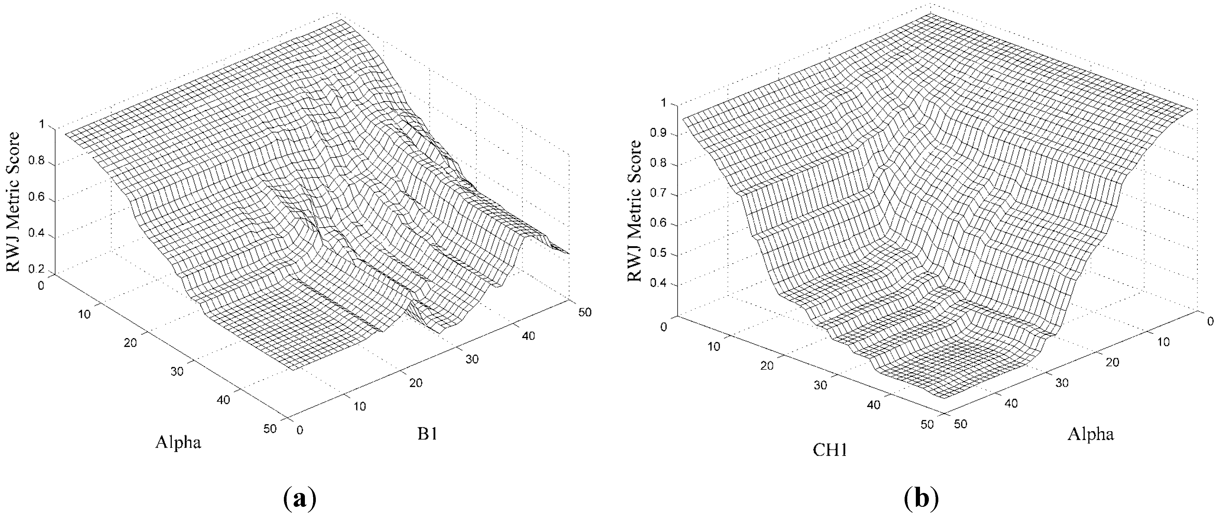
Figure 8 shows exhaustive fitness calculations (RWJ metric) for arbitrary two-dimensional slices of the parameter space (also called the search surface).
Figure 8a shows the interaction of the local range parameter of the CC algorithm interacting with the B1 parameter of the spectral split mapping function. Note two local optima. All other parameters were given initial random values and were kept constant during the generation of the search surface.
Figure 8b illustrates similarly, with a simpler interaction (single optimal) between thresholds of the CH1 attribute and the local range parameter of CC. Note that these figures are illustrative of parameter interactions and may be vastly different (more complex/less complex) under different external parameter conditions.
5.2. Search Surface Complexity
In
Section 5.1, it was shown that parameter interactions exist in the presented method. Some interactions are frequent in the case of selected constituents. Here we investigate the applicability [
39] of a range of search methods to traverse the search surfaces of the four method variants. Intuitively the CC variant of the method, with a relatively simple interaction between the local and global range parameters, would not be a difficult search problem. Simple parameter tuning would be feasible in such a scenario using the CC variant of the method, or a simple grid search or random parameter search.
Figure 8.
Two-dimensional parameter plots, or search surfaces, demonstrating parameter interactions between method constituents: (a) illustrates the interaction of the alpha parameter from the CC constituent and that of a mapping function parameter, while (b) shows the interaction of alpha with the CH1 attribute.
The four method variants are run on the Bokolmanyo problem (GT mapping), conjectured to exhibit the simplest search surfaces. Four search methods, namely random search (RND), HillClimber (HC), standard particle swarm optimization (PSO), and a standard variant of Differential Evolution (DE) are investigated (
Section 2.3). The RWJ metric is used to judge segment quality. The search process is granted 2000 iterations. Thus, although the tested search methods have vastly different mechanisms (single or population-based, stochastic or deterministic), they are evaluated based on an equal computing budget. Each experiment is repeated 20 times. Averages over the 20 runs are quoted, with the standard deviations also given. The CC method variant has a two-dimensional parameter domain, the CC + Attr variant 12 dimensions, CC + Map also 12 and the CC + Attr + Map method variant 22. Cross-validation was not performed, as search method progress and feasibility were evaluated.
Table 7 lists the optimal achieved metric scores (RWJ) given 2000 search method iterations. The shaded cells indicate the search methods achieving the best scores for each method variant. Various ties in optimal results among the search methods are noted. Firstly, on examining the CC method variant, as expected, no benefit is seen from using more complex search methods. Note that even on this simple search surface, the HC method could not find the global optimal routinely. Similarly, adding attribute thresholding as additional parameters (CC + Attr) gave similar results across the different search methods. Again, HC performed worse than the other methods. In these two method variants, RND, PSO, and DE routinely generated the optimal results. Note that initialization of the parameters in the search processes was random (as opposed to, for example, distributed hypercube sampling). Interestingly, none of the search methods was able to find optimal values on the edge of the search domain when attributes were introduced (owing to random initialization).
Table 7.
Performance of the four search methods on the four method variants. In the simpler CC method variants (CC and CC + Attr), no benefit is noted from using more advanced search methods. In the case of the higher dimensional method variants (CC + Map and CC + Attr + Map), using an advanced search method becomes necessary.
| | CC | CC + Attr | CC + Map | CC + Attr + Map |
|---|
| RND | 0.429 ± 0.000 | 0.448 ± 0.000 | 0.186 ± 0.012 | 0.193 ± 0.015 |
| HC | 0.442 ± 0.009 | 0.535 ± 0.144 | 0.507 ± 0.083 | 0.538 ± 0.159 |
| PSO | 0.429 ± 0.000 | 0.448 ± 0.000 | 0.167 ± 0.012 | 0.163 ± 0.008 |
| DE | 0.429 ± 0.000 | 0.448 ± 0.000 | 0.161 ± 0.003 | 0.163 ± 0.003 |
Considering the CC + Map and CC + Attr + Map variants of the method, the more complex search methods (PSO, DE) performed substantially better (statistically significantly different, Student’s
t-test with a 95% confidence interval) than the RND and especially the HC search method. A difference in 0.030 in the case of the RWJ metric when results approach their optimum is in a practical sense very noticeable. This suggests that under the higher dimensional problem conditions, with more complexities introduced by a mapping function, stochastic population-based search strategies (or others) are needed. Note the slight decrease in standard deviation in the most complex method variants. Also, as generally documented [
60], the generic variant of DE performed slightly better than the generic variant of PSO. Further results are presented exclusively with the DE method.
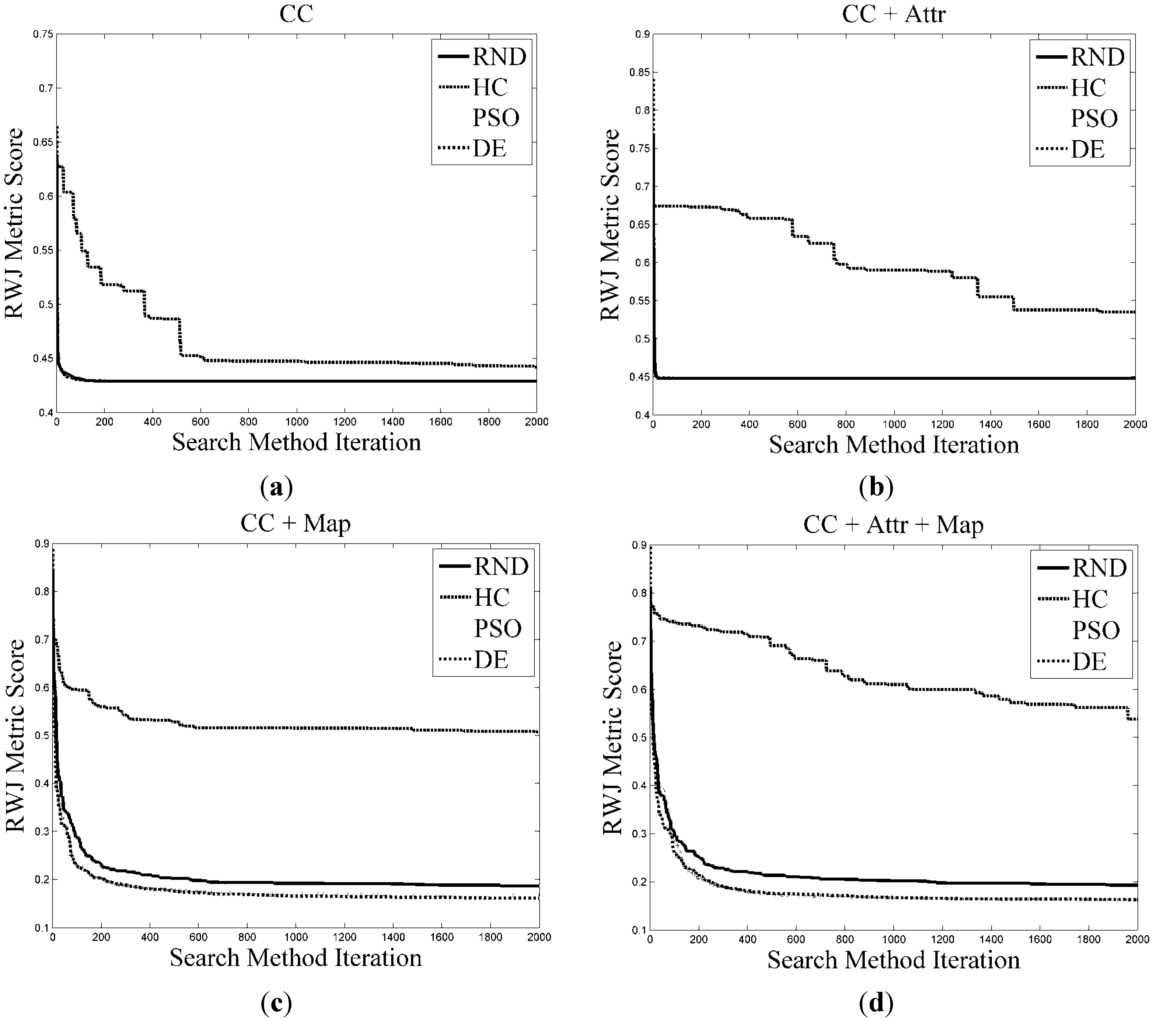
Figure 9 shows the search progress profiles over the allocated 2000 iterations (averaged over 20 runs) for the CC (
Figure 9a), CC + Attr (
Figure 9b), CC + Map (
Figure 9c), and CC + Attr + Map (
Figure 9d) method variants. Note that in the simpler method variants (CC and CC + Attr), the optimal results are achieved within 100 method iterations. The more complex method variants (CC + Map and CC + Attr + Map) need substantially more search iterations to achieve optimal or near-optimal results.
Figure 9c,d also shows that under the more complex problem formulations, PSO and DE provide better results relatively early on in the search process, suggesting their use even under constrained processing conditions. These plots reveal that method termination may be suggested at around 1000 iterations in these method formulations, or an alternative termination condition may be encoded based on derivatives observed between 500 and 1000 iterations.
Figure 9.
Search method profiles for the four method variants, namely CC (a), CC + Attr (b), CC + Map (c), and CC + Attr + Map (d). Note the increased performance of DE and PSO when considering the CC + Map and CC + Attr + Map method variants.
Figure 9.
Search method profiles for the four method variants, namely CC (a), CC + Attr (b), CC + Map (c), and CC + Attr + Map (d). Note the increased performance of DE and PSO when considering the CC + Map and CC + Attr + Map method variants.
5.3. Method Variant Performances
The four presented method variants are evaluated, relative to one another, based on maximal achieved metric scores under cross-validated conditions. Profiling such relative performances in general may give an indication of the merits of the constituents in such a framework. Computing times are also contrasted, as well as convergence behavior, which are important considerations to reduce method processing times. For each problem (Bokolmanyo, Jowhaar, Hagadera), the four method variants are run using all three detailed empirical discrepancy metrics. Each experiment is repeated 20 times, with averages and standard deviations reported. For each site a random mapping function was selected (SS, LIN, or GT). In addition, the best results obtained during the 20 runs are also reported. Thus for each method variant, nine differentiated segmentation tasks (problem type, metric characteristic) are evaluated with over 50 million individual segment evaluations conducted.
Table 8,
Table 9 and
Table 10 list the achieved metric scores for the problems under different metric and method variant conditions. Note that method variants may be contrasted based on a given metric and not via different metric values. On examining
Table 8, depicting the Bokolmanyo problem, it is clear that the more elaborate method variants employing a mapping function (LIN in this case) and a mapping function plus attributes generated superior results compared with the CC and CC + Attr variants. Interestingly, under cross-validated conditions, the addition of constraining attributes (CC + Attr) created an overfitting scenario, resulting in worse performances compared with not employing constraining attributes.
The performances of CC + LIN and CC + Attr + LIN are similar, with the given metric dictating the superior method. Under the RBSB metric condition the CC + LIN method variant displays extremely sporadic results. This suggests that the search surfaces generated under this condition contain numerous discontinuities, creating difficulties for the DE search method. This may be due to the formulation, or nature, of RBSB. It is reference segment centric. In contrast, considering the CC + Attr method variant, the RBSB metric proved robust and similar to the CC variant in terms of optimal results.
Table 8.
Method performance on the Bokolmanyo problem. Note the improved results with the CC + LIN and CC + Attr + LIN method variants under all metric conditions.
Table 8.
Method performance on the Bokolmanyo problem. Note the improved results with the CC + LIN and CC + Attr + LIN method variants under all metric conditions.
| | | CC | CC + Attr | CC + LIN | CC + Attr + LIN |
|---|
| RWJ | Avg | 0.465 ± 0.000 | 0.520 ± 0.035 | 0.239 ± 0.020 | 0.235 ± 0.026 |
| Min | 0.465 | 0.476 | 0.211 | 0.200 |
| RBSB | Avg | 0.299 ± 0.000 | 0.308 ± 0.009 | 0.262 ± 0.235 | 0.185 ± 0.034 |
| Min | 0.299 | 0.301 | 0.136 | 0.144 |
| PD_OCE | Avg | 0.538 ± 0.009 | 0.556 ± 0.030 | 0.233 ± 0.016 | 0.244 ± 0.026 |
| Min | 0.526 | 0.514 | 0.199 | 0.205 |
The Jowhaar problem (
Table 9) displays a slightly different general trend. Under all metric conditions the mapping function method variant (CC + SS) proved superior to both the attribute (CC + Attr) and combined mapping function and attribute (CC + Attr + SS) method variants. Under cross-validated conditions, no benefit was seen from employing attributes, commonly leading to worse results. Note that generally the absolute results were poorer compared with the easier Bokolmanyo problem.
Table 9.
Method performance on the Jowhaar problem. The method variant employing a data mapping function (CC + SS) performed the best under all metric conditions.
Table 9.
Method performance on the Jowhaar problem. The method variant employing a data mapping function (CC + SS) performed the best under all metric conditions.
| | | CC | CC + Attr | CC + SS | CC + Attr + SS |
|---|
| RWJ | Avg | 0.551 ± 0.003 | 0.784 ± 0.001 | 0.411 ± 0.009 | 0.757 ± 0.013 |
| Min | 0.548 | 0.783 | 0.392 | 0.739 |
| RBSB | Avg | 0.622 ± 0.000 | 0.652 ± 0.003 | 0.418 ± 0.058 | 0.616 ± 0.023 |
| Min | 0.622 | 0.649 | 0.348 | 0.581 |
| PD_OCE | Avg | 0.684 ± 0.002 | 0.825 ± 0.006 | 0.549 ± 0.032 | 0.807 ± 0.021 |
| Min | 0.683 | 0.816 | 0.506 | 0.769 |
The Hagadera problem (
Table 10), considered the most difficult problem, exhibits curious results not corroborating trends observed in the previous two problems. Under different metric conditions, the three method variants (CC + Attr, CC + GT, and CC + Attr + GT) all achieved the top performance. CC + GT was superior under the RWJ metric condition, CC + Attr under the RBSB condition, and CC + Attr + GT under the PD_OCE condition.
Table 10.
Method performances on the Hagadera problem. The top performing method variant is metric dependent.
Table 10.
Method performances on the Hagadera problem. The top performing method variant is metric dependent.
| | | CC | CC + Attr | CC + GT | CC + Attr + GT |
|---|
| RWJ | Avg | 0.614 ± 0.000 | 0.631 ± 0.008 | 0.492 ± 0.013 | 0.509 ± 0.012 |
| Min | 0.614 | 0.619 | 0.468 | 0.494 |
| RBSB | Avg | 0.737 ± 0.000 | 0.511 ± 0.014 | 1.633 ± 1.061 | 0.522 ± 0.045 |
| Min | 0.737 | 0.486 | 0.526 | 0.460 |
| PD_OCE | Avg | 0.705 ± 0.001 | 0.684 ± 0.005 | 0.617 ± 0.023 | 0.616 ± 0.028 |
| Min | 0.704 | 0.678 | 0.579 | 0.553 |
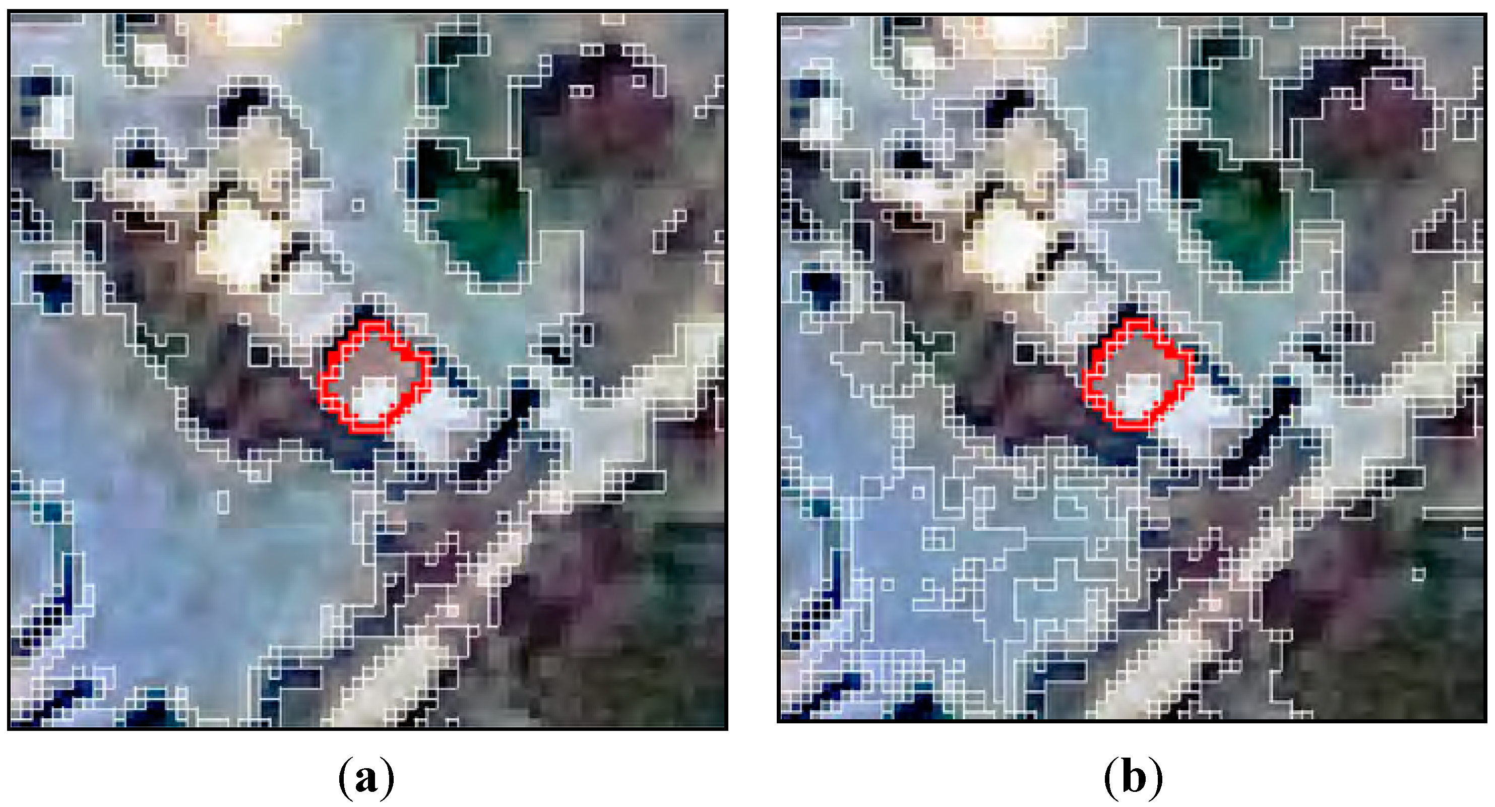
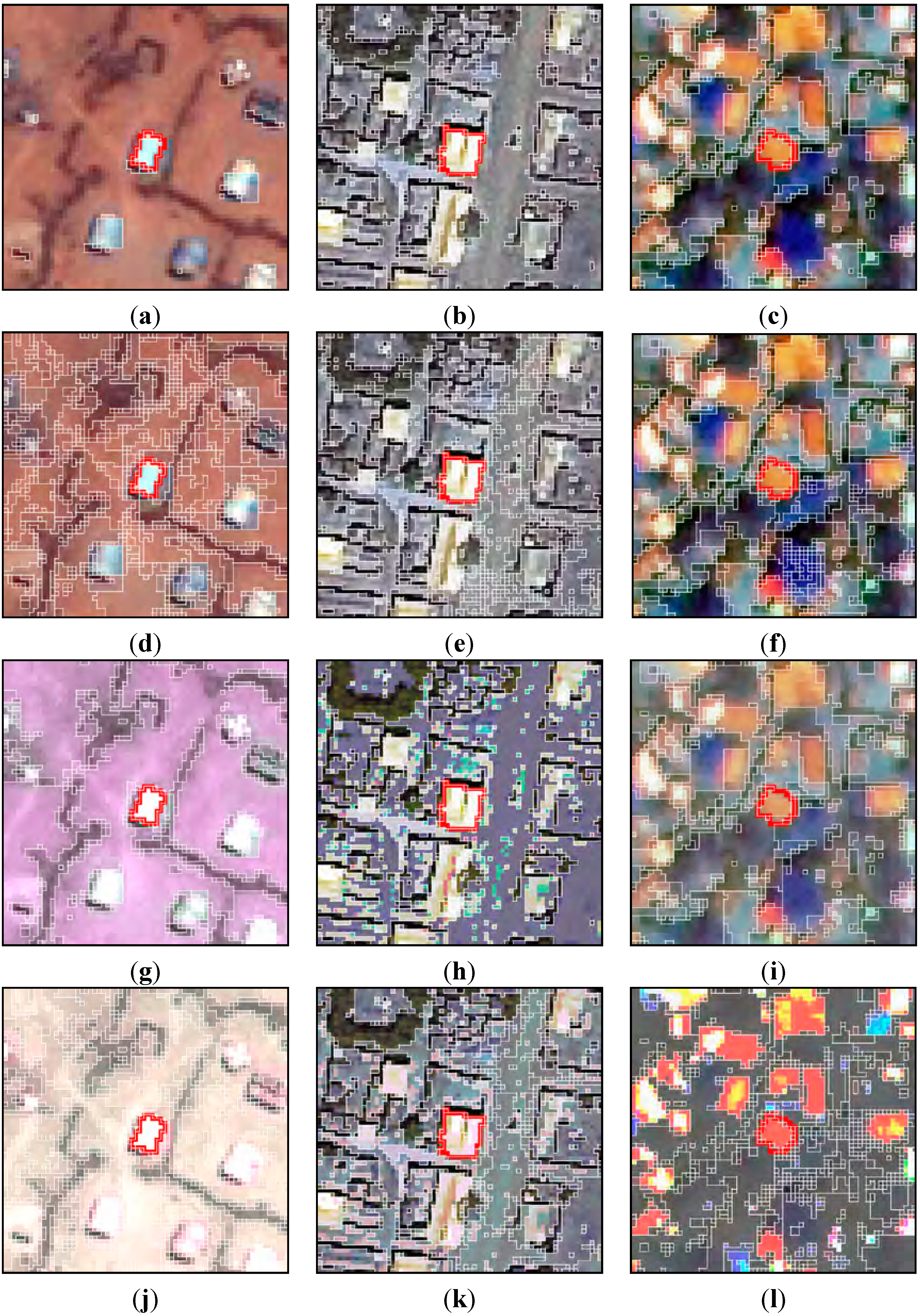
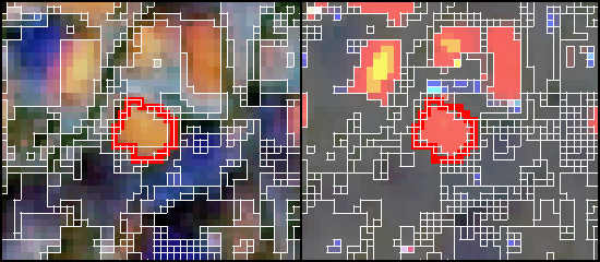
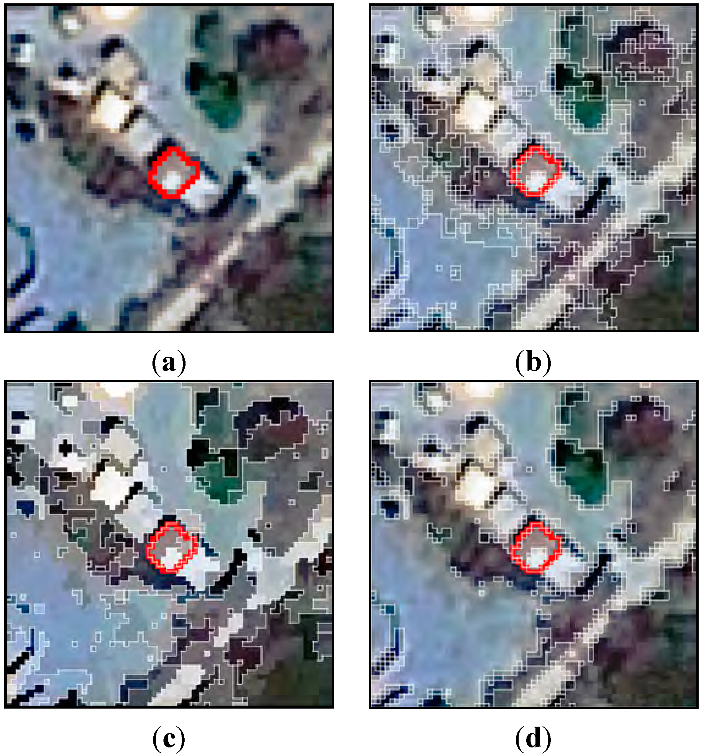
Figure 10 shows some optimal results obtained for various problem runs depicted in
Table 8,
Table 9 and
Table 10. Each sub-figure shows a given reference segment, delineated with a red polyline. Resulting segments for the best performing parameter sets are shown with white polylines. The RWJ metric scores for the specific segment are also quoted. The given metric scores are specific to the red delineated reference segments shown (randomly chosen) and not the averaged and cross-validated results generated during experimentation.
Figure 10a–c shows local optimal results for the CC method variant.
Figure 10d–f presents the results under the CC + Attr method variant,
Figure 10g–i for the CC + Map method variant and
Figure 10j–l for the CC + Attr + Map variant. Note the same results generated for the Jowhaar problem under CC and CC + Attr method conditions (
Figure 10b,e), with constraining attributes not affecting segment quality over the given reference segment.
Generally, based on observing
Table 8,
Table 9 and
Table 10, the introduction of mapping functions provides more robust improvements under more conditions compared with adding attributes. In some cases a combination of attributes and a mapping function proved most useful.
Table 11 lists the average computing times needed for 2000 method evaluations, contrasting the performances of the CC + Map and CC + Attr method variants. Computing attributes requires substantially more computing time (Intel
® Xeon
® E5-2643 3.5 GHz processor with single-core processing). Attribute calculations were done incrementally in the CC framework, which is more efficient than calculating attributes independently for each new level of the local range parameter. The optimal achieved parameter values are also reported. Similar to related work [
6], near optimal parameter value combinations exist owing to segmentation algorithm and mapping function characteristics.
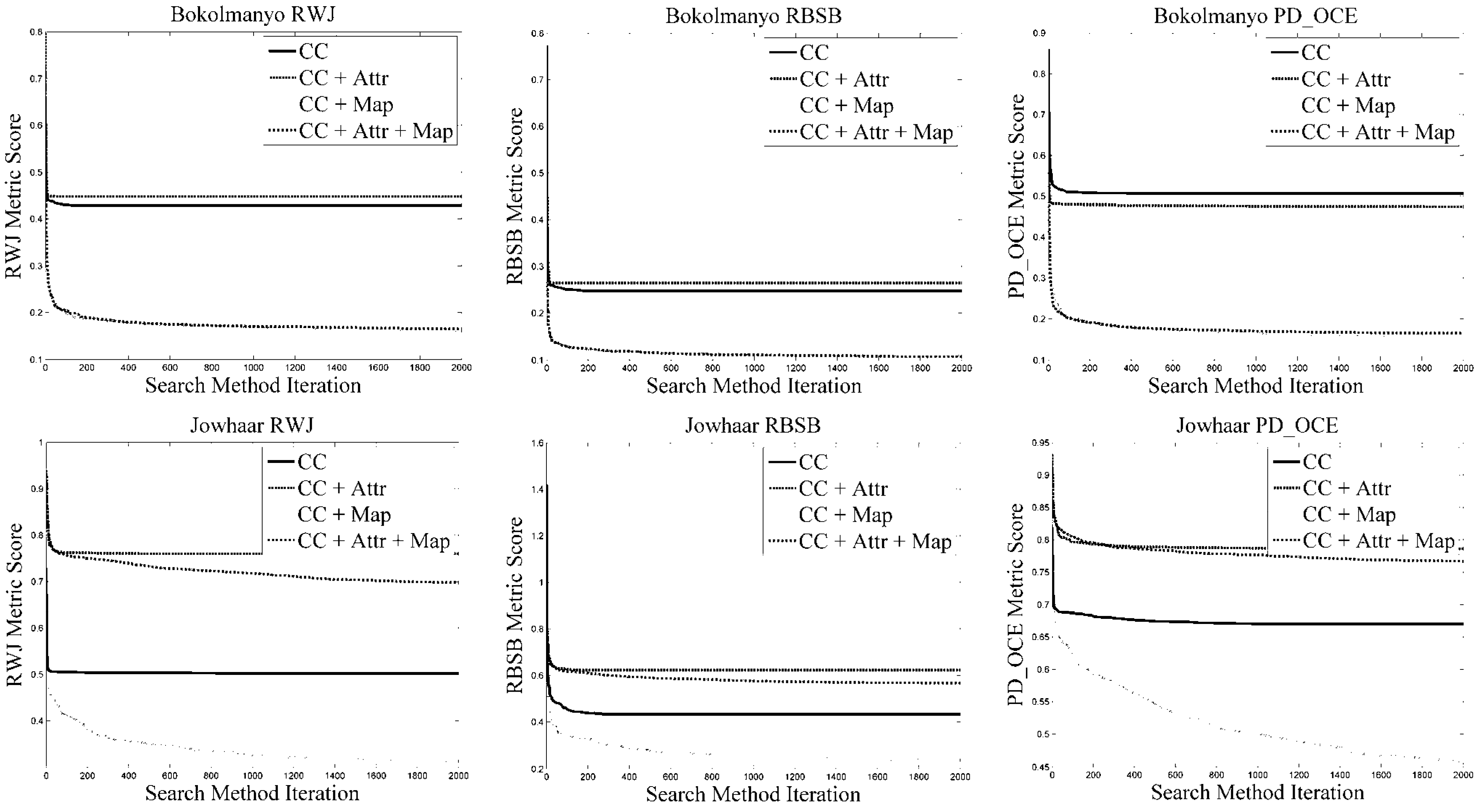
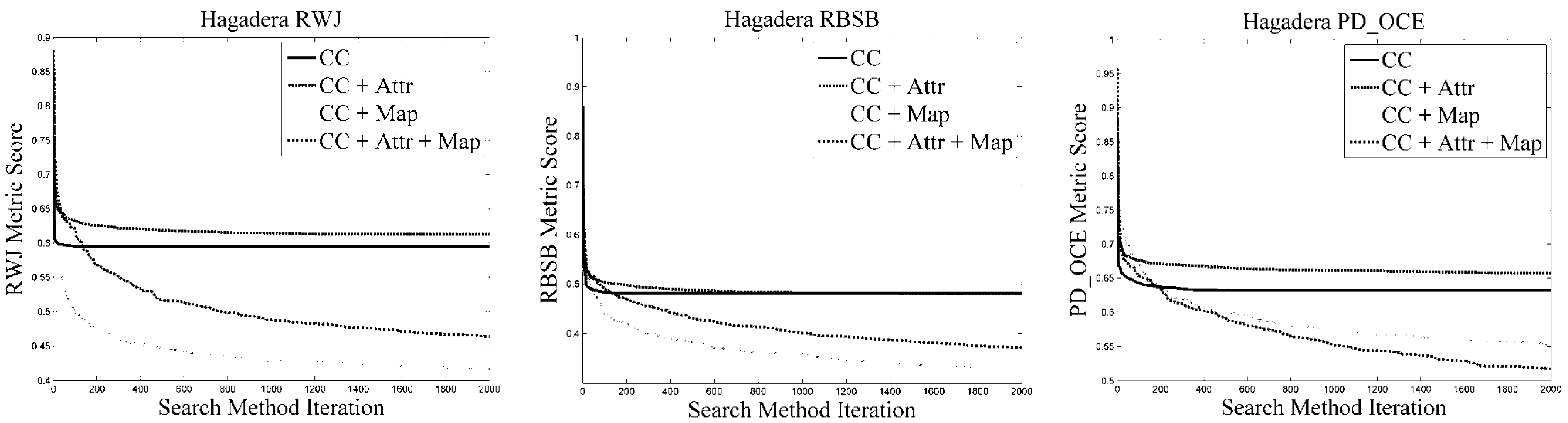
Following on from
Table 11,
Figure 11 shows the averaged fitness profiles for the various problems and corresponding metrics, prior to cross-validation. Specifically, note the slightly slower start of mapping function method variants compared with attribute variants; however, they ultimately lead to better results (and in the first two problems start off better). In terms of search method progression, some variation exists based on the difficulty of the problem. Generally all variants converged more slowly in the Hagadera problem (“difficult”) compared with the Bokolmanyo problem. Note the variations in optimal results compared with cross-validated values (
Table 8,
Table 9 and
Table 10), specifically considering the RBSB metric with its compact formulation. The figure also highlights the fact that the more complex method variants obtain superior results relatively quickly in the search processes—useful information if method execution times need to be short.
Figure 10.
Exemplar optimal segmentation results focused on a random reference segment. The rows depict the CC, CC + Attr, CC + Map, and CC + Attr + Map method variants respectively (in order). The columns denote the three problems, Bokolmanyo, Jowhaar, and Hagadera (in order). (a) RWJ: 0.574; (b) RWJ: 0.524; (c) RWJ: 0.787; (d) RWJ: 0.683; (e) RWJ: 0.524; (f) RWJ: 0.806; (g) RWJ: 0.104; (h) RWJ: 0.506; (i) RWJ: 0.787; (j) RWJ: 0.063; (k) RWJ: 0.437; (l) RWJ: 0.549.
Table 11.
Average computing times for experimental runs and resulting method parameters. Note the increased computing time of method variants employing attributes.
Table 11.
Average computing times for experimental runs and resulting method parameters. Note the increased computing time of method variants employing attributes.
| Problem | Method Variant | Time | Alpha | WGlobal | Area | Std | Perimeter | Smoothness | Compactness |
|---|
| Bokolmanyo | CC + Map | 2062.304 ± 248.996 | 187.600 ± 68.646 | 53.600 ± 15.601 | NA | NA | NA | NA | NA |
| | CC + Attr | 3083.551 ± 237.328 | 173.300 ± 66.331 | 196.000 ± 44.838 | 247.500 ± 142.417 | 50.442 ± 58.470 | 369.900 ± 196.794 | 21.483 ± 7.688 | 19.803 ± 7.439 |
| Jowhaar | CC + Map | 2182.659 ± 193.999 | 165.900 ± 82.538 | 155.200 ± 19.136 | NA | NA | NA | NA | NA |
| | CC + Attr | 4136.116 ± 498.270 | 98.900 ± 52.297 | 203.500 ± 43.775 | 392.000 ± 85.249 | 133.289 ± 60.647 | 620.500 ± 241.420 | 18.379 ± 6.910 | 22.466 ± 4.331 |
| Hagadera | CC + Map | 2168.177 ± 226.159 | 101.700 ± 65.052 | 148.300 ± 29.803 | NA | NA | NA | NA | NA |
| | CC + Attr | 5409.293 ± 352.444 | 187.400 ± 68.704 | 240.300 ± 21.525 | 342.100 ± 81.266 | 162.601 ± 86.782 | 574.700 ± 271.998 | 23.573 ± 7.351 | 19.940 ± 6.113 |
Finally, and most significantly, the results reported in
Table 8,
Table 9 and
Table 10 are augmented with a Friedman rank test [
61] to give a generalized and discrete indication of the usefulness of the method variants. The Friedman rank test is a simple non-parametric test ranking multiple methods (e.g., CC, CC + Map,
etc.) over multiple problems/data sets. The rank test was run on the four method variants considering the various problems and metric conditions (36 in total, cross-validated). A Nemenyi
post hoc test was also conducted to test whether critical differences exist.
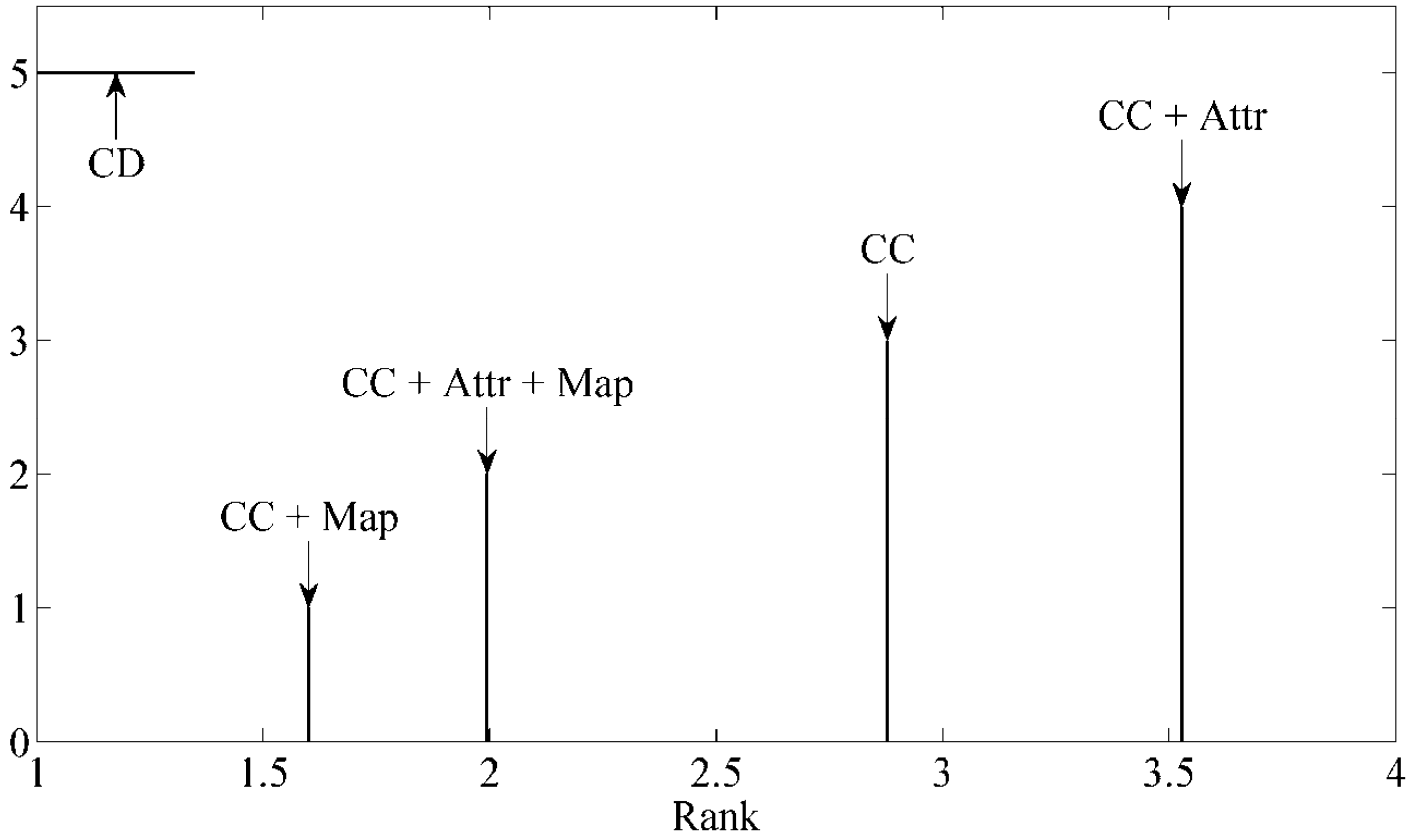
Figure 12 illustrates this result, with the confidence interval set to 95% and a critical difference of 0.349 (ranking) generated. Note that the figure shows results under cross-validated conditions.
Figure 11.
Search method profiles for the different problems under different metric conditions. Note that for the simpler Bokolmanyo problem near-optimal results are achieved relatively early on in the search process. In the more complex problems, the methods need substantially more iterations in finding the achievable optimal parameter set.
On examining
Figure 12, the CC + Map variant of the method (using various mapping functions) ranked first, followed by the most complex method variant (CC + Attr + Map). Under cross-validated conditions, adding attributes proves detrimental. The investigated problems are not exhaustive. The variants are all statistically significantly different from one another. This figure reports a general observation under extensive evaluations (50 million segment evaluations). Under a more succinct selection of attributes and problems, attributes may well be more useful. The figure suggests simple data mapping functions should be a worthwhile consideration in method design within this general framework. Mapping functions may be considered (indirect means of changing connectivity type), but other more direct means of defining connectivity (parameterizable) may also prove useful. This is in addition to such a variant requiring less computing time, compared with computing additional attributes.
Figure 12.
Friedman rank test with a Nemenyi
post hoc test conducted on results from
Table 8,
Table 9 and
Table 10. Confidence interval is set to 95%. A Critical Difference (CD) of 0.349 is generated (ranking). All method variants deliver statistically significant different results. Generally speaking, the CC + Map method variant was found most useful.


