
Toward Improved Daily Cloud-Free Fractional Snow Cover Mapping with Multi-Source Remote Sensing Data in China


Abstract
:
1. Introduction
2. Data
2.1. MODIS FSC Product
2.2. AMSR2 Snow Water Equivalent (SWE) Product
2.3. Landsat 8 OLI Data

| Band No. | Band | Bandwidth (μm) | Spatial Resolution (m) | Radiometric Resolution (bit) |
|---|---|---|---|---|
| 1 | Coastal aerosol | 0.433–0.453 | 30 | 12 |
| 2 | Blue | 0.450–0.515 | 30 | 12 |
| 3 | Green | 0.525–0.600 | 30 | 12 |
| 4 | Red | 0.630–0.680 | 30 | 12 |
| 5 | Near Infrared | 0.845–0.885 | 30 | 12 |
| 6 | SWIR 1 | 1.560–1.660 | 30 | 12 |
| 7 | SWIR 2 | 2.100–2.300 | 30 | 12 |
| 8 | Panchromatic | 0.500–0.680 | 15 | 12 |
| 9 | Cirrus | 1.360–1.390 | 30 | 12 |
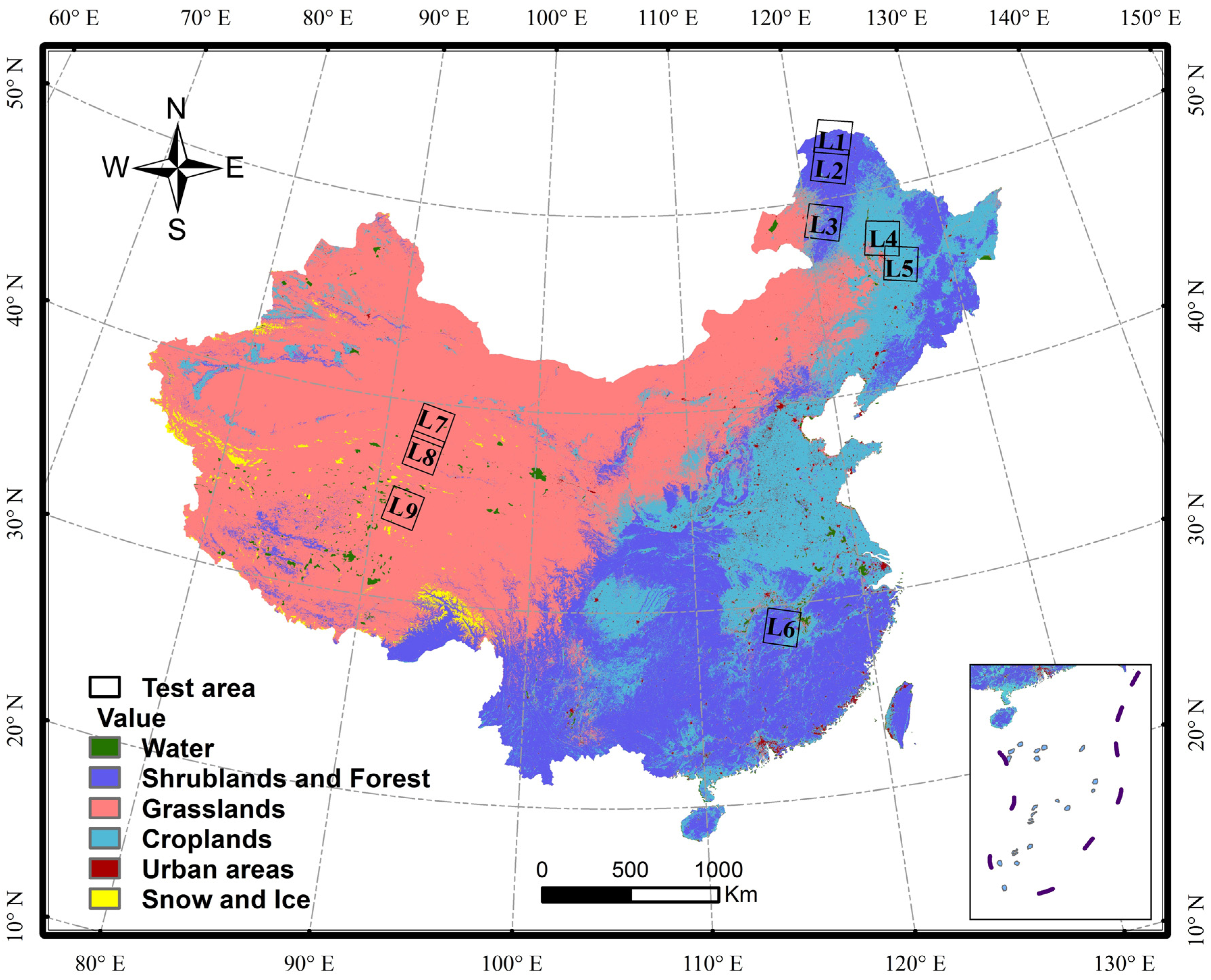
| Number | Date | Main Land Cover Types | Strip Number | Line Number | Cloud (%) |
|---|---|---|---|---|---|
| L1 | 16 January 2014 | Shrublands and Forest | 122 | 23 | 3.18 |
| L2 | 16 January 2014 | Shrublands and Forest | 122 | 24 | 6.10 |
| L3 | 16 January 2014 | Shrublands and Forest | 122 | 26 | 8.55 |
| L4 | 26 December 2014 | Cropland | 119 | 27 | 3.07 |
| L5 | 5 February 2014 | Cropland | 118 | 28 | 9.10 |
| L6 | 16 January 2014 | Cropland | 122 | 40 | 4.81 |
| L7 | 16 January 2014 | Grasslands | 138 | 33 | 4.48 |
| L8 | 16 January 2014 | Grasslands | 138 | 34 | 6.62 |
| L9 | 16 January 2014 | Grasslands | 138 | 36 | 5.04 |
2.4. IGBP Land Cover Type Product
2.5. SRTM Digital Elevation Model (DEM)

3. Methodology
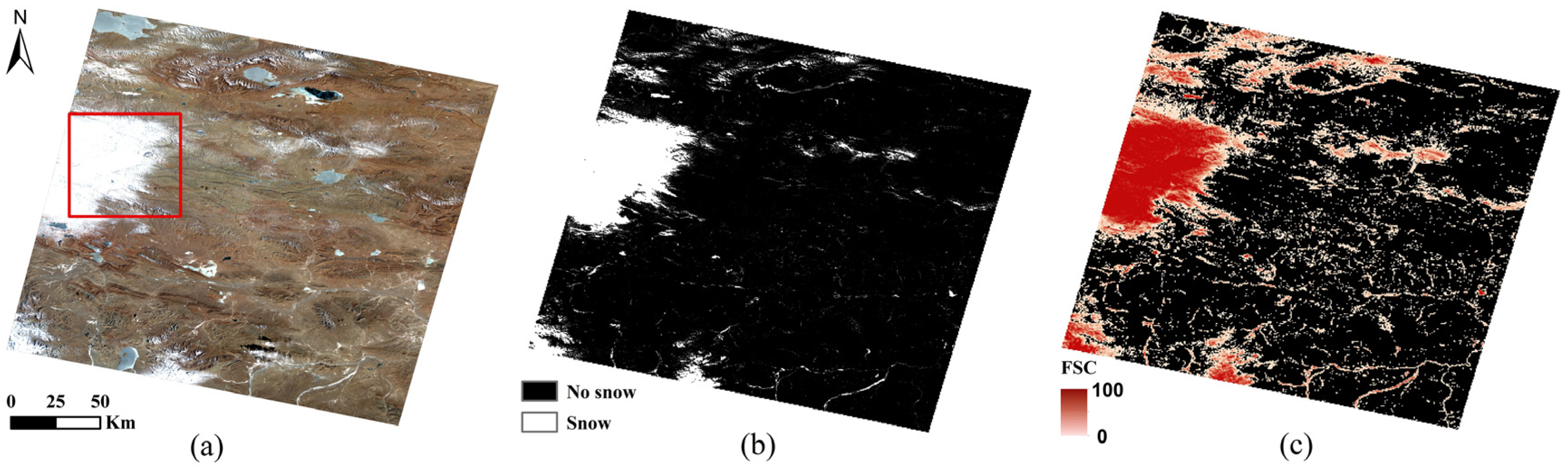
3.1. OLI Snow Mapping

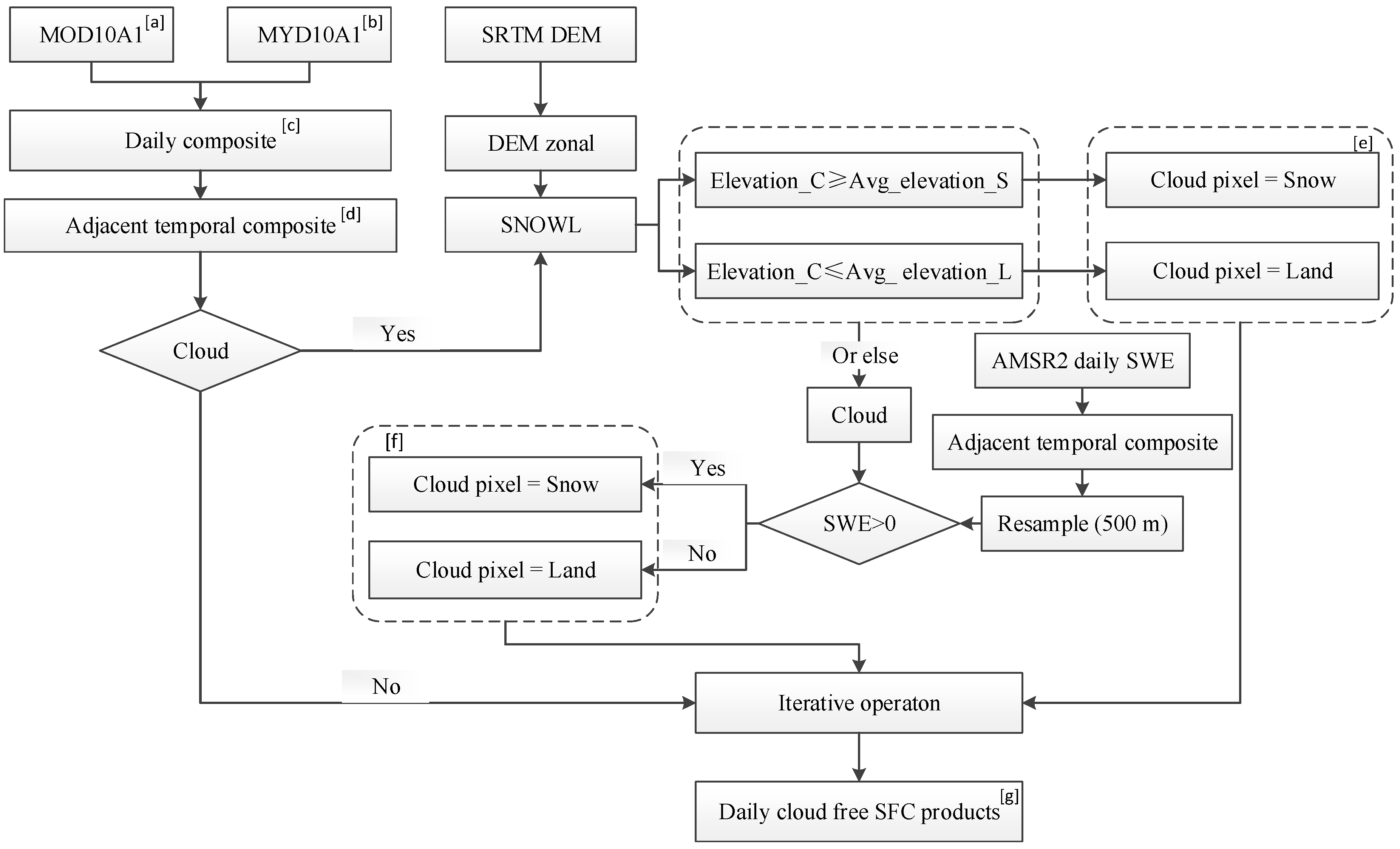
3.2. Cloud Removal Algorithm
3.2.1. Daily Composite
| MOD10A1 Code Values | MYD10A1 Code Values | |||||
|---|---|---|---|---|---|---|
| 0–100 | 225 | 237 | 239 | 250 | 200\201\254\255 * | |
| 0–100 (Snow) | (MOD + MYD) × 0.5 | MOD | MOD | MOD | MOD | MOD |
| 225 (Land) | MYD | 225 | 225 | 225 | 225 | 225 |
| 237 (Inland water) | MYD | 237 | 237 | 237 | 237 | 237 |
| 239 (Ocean) | MYD | 239 | 239 | 239 | 239 | 239 |
| 250 (Cloud) | MYD | 225 | 237 | 239 | 250 | 250 |
| 200\201\254\255 * | MYD | 225 | 237 | 239 | 250 | 200\201\254\255 |
3.2.2. Adjacent Temporal Composite
3.2.3. Snow Line Algorithm (SNOWL)
3.2.4. Composite with AMSR2 SWE
3.2.5. Iterative Operation
3.3. Validation
4. Results
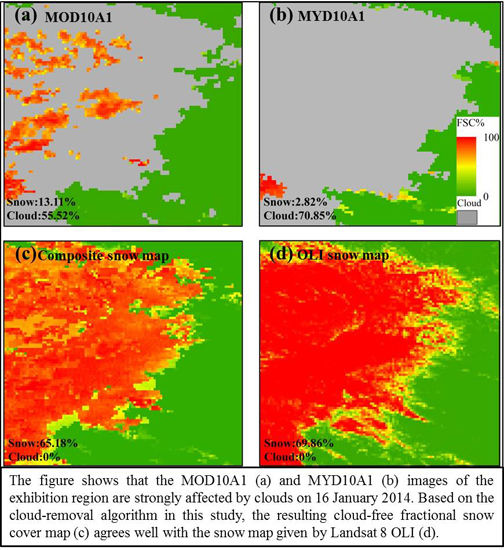
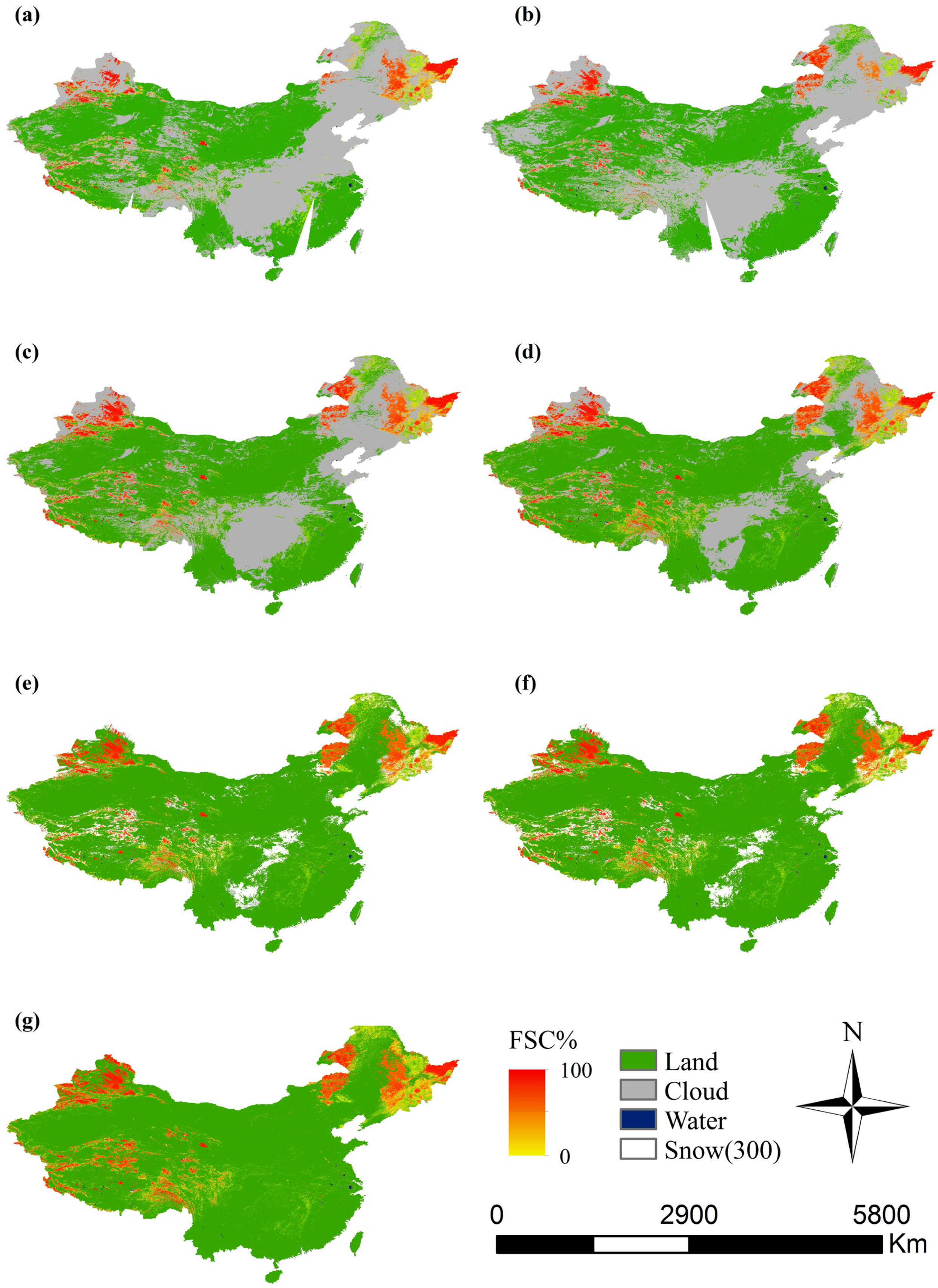
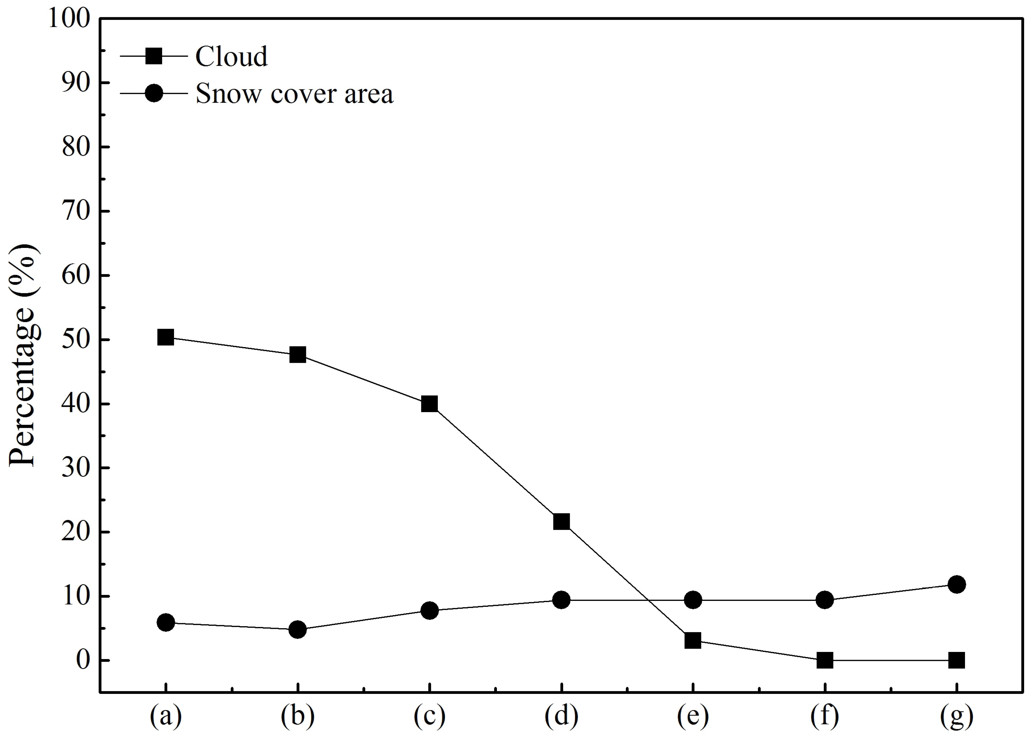
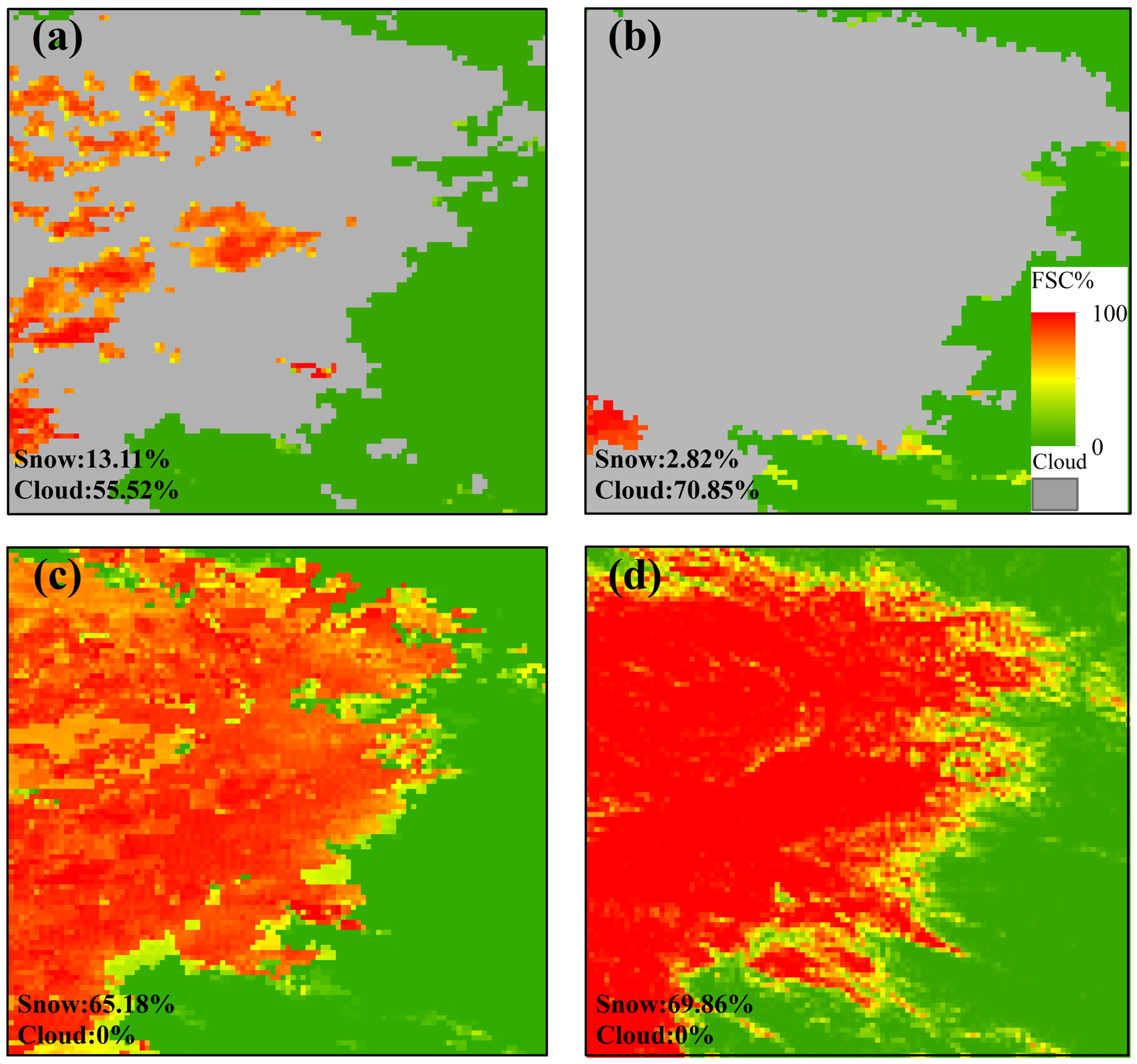
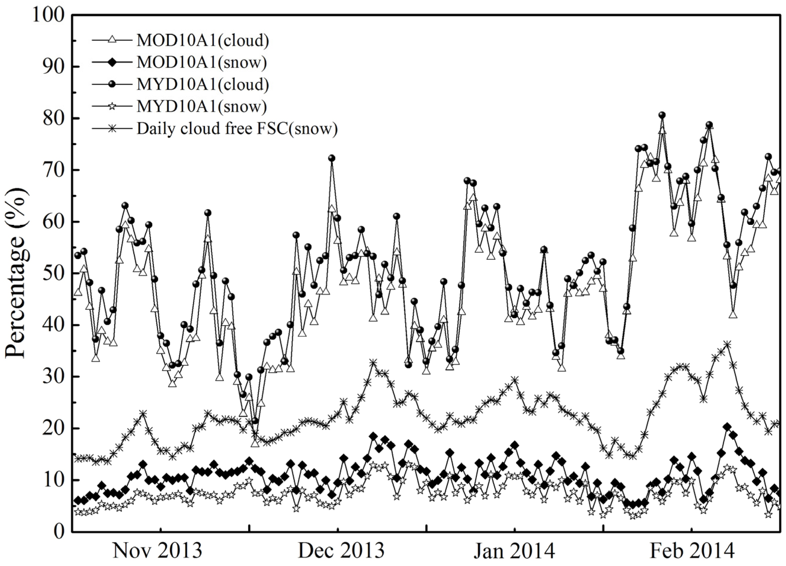
4.1. Effect of Cloud Removal


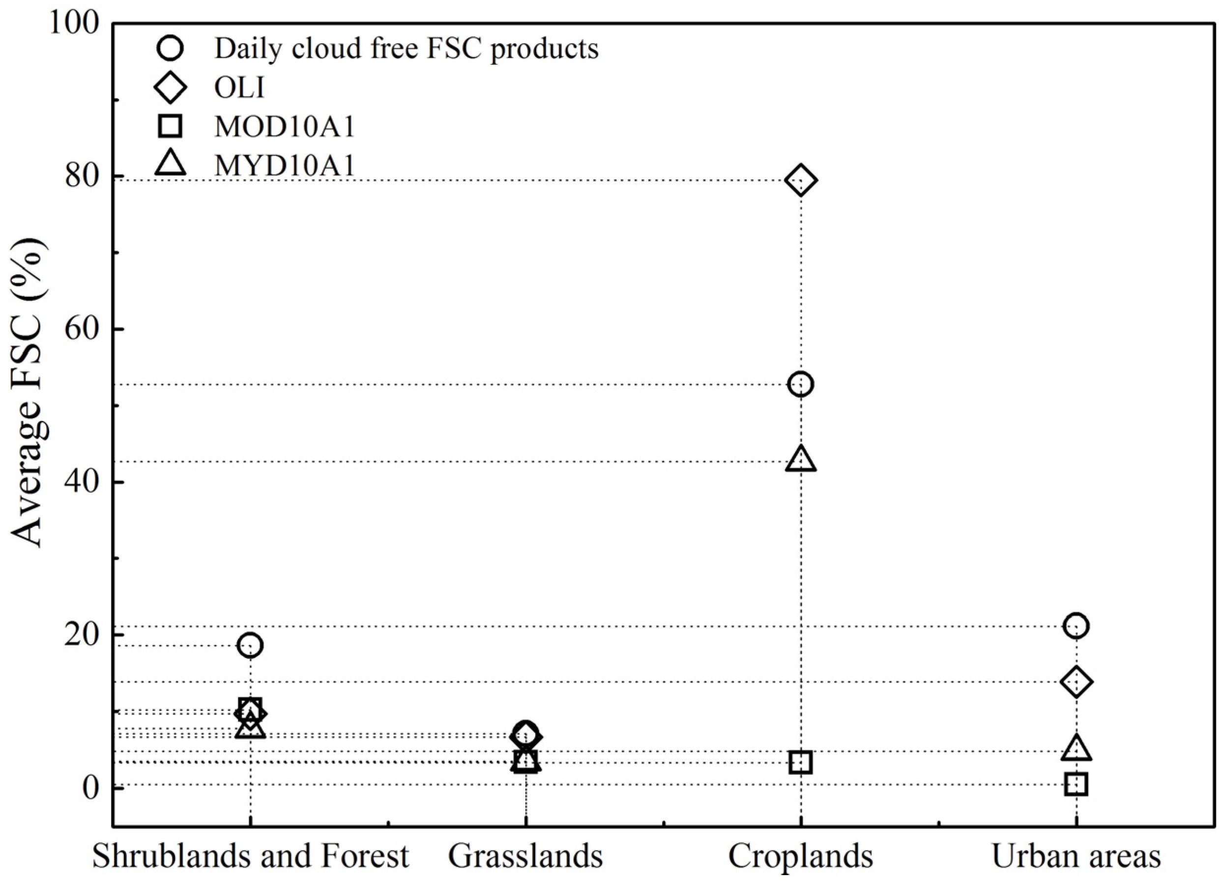
4.2. Accuracy Test of the Daily Cloud-Free FSC Product


| Land Cover Types | MAE | RMSE | R2 |
|---|---|---|---|
| Shrublands and Forest | 0.21 | 0.28 | 0.40 |
| Grasslands | 0.04 | 0.13 | 0.91 |
| Croplands | 0.32 | 0.46 | 0.82 |
| Urban areas | 0.22 | 0.32 | 0.65 |
| Overall | 0.20 | 0.29 | 0.70 |
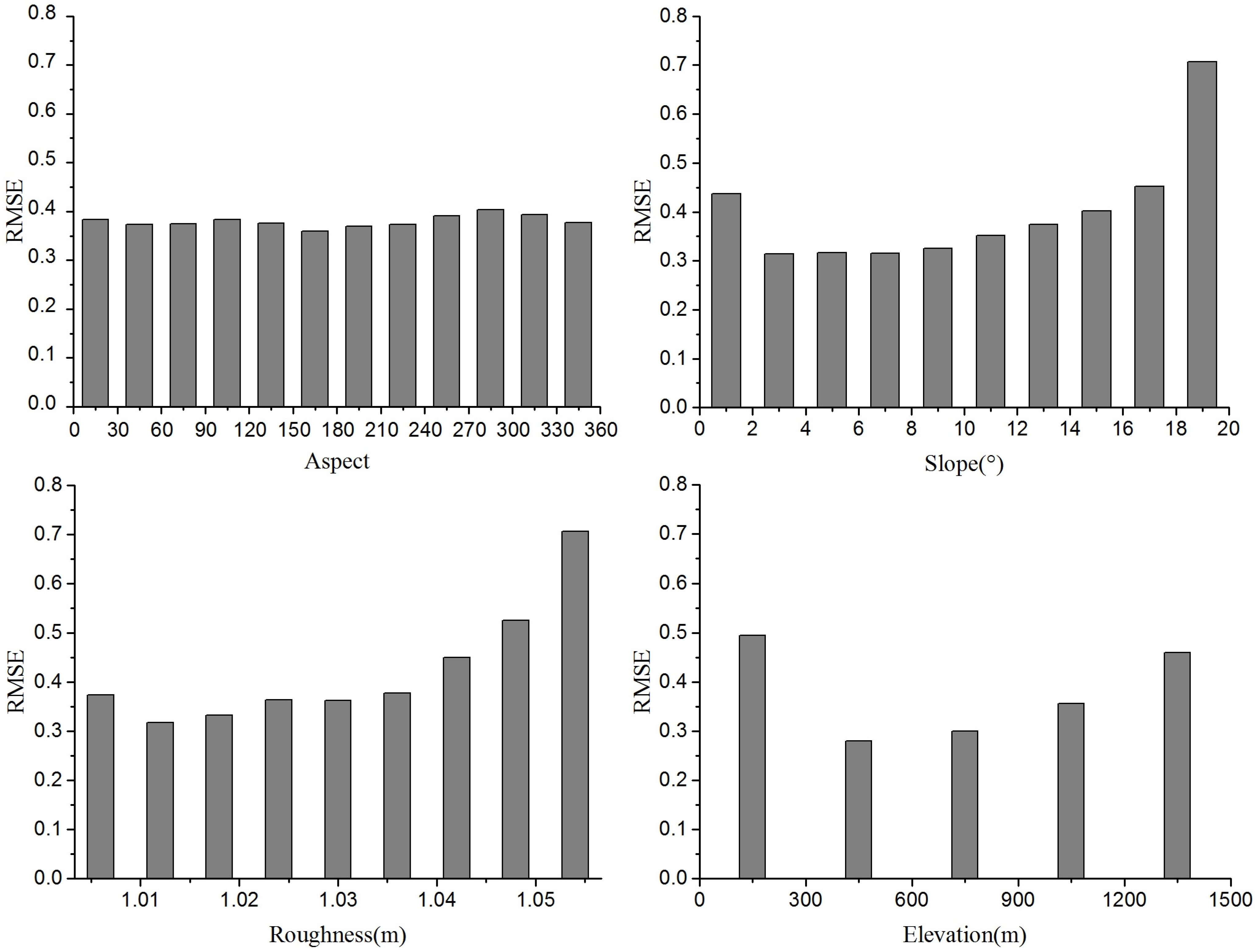
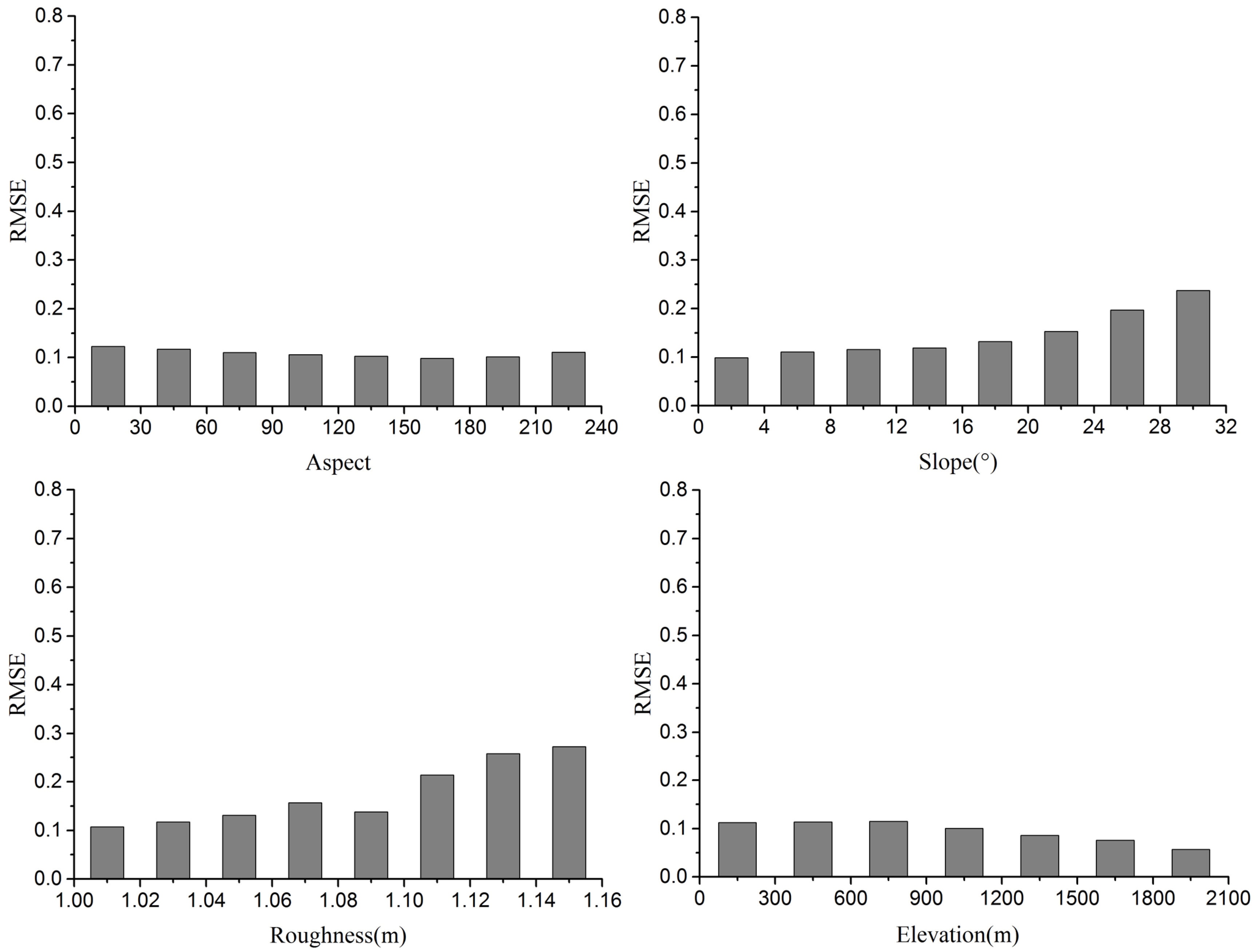
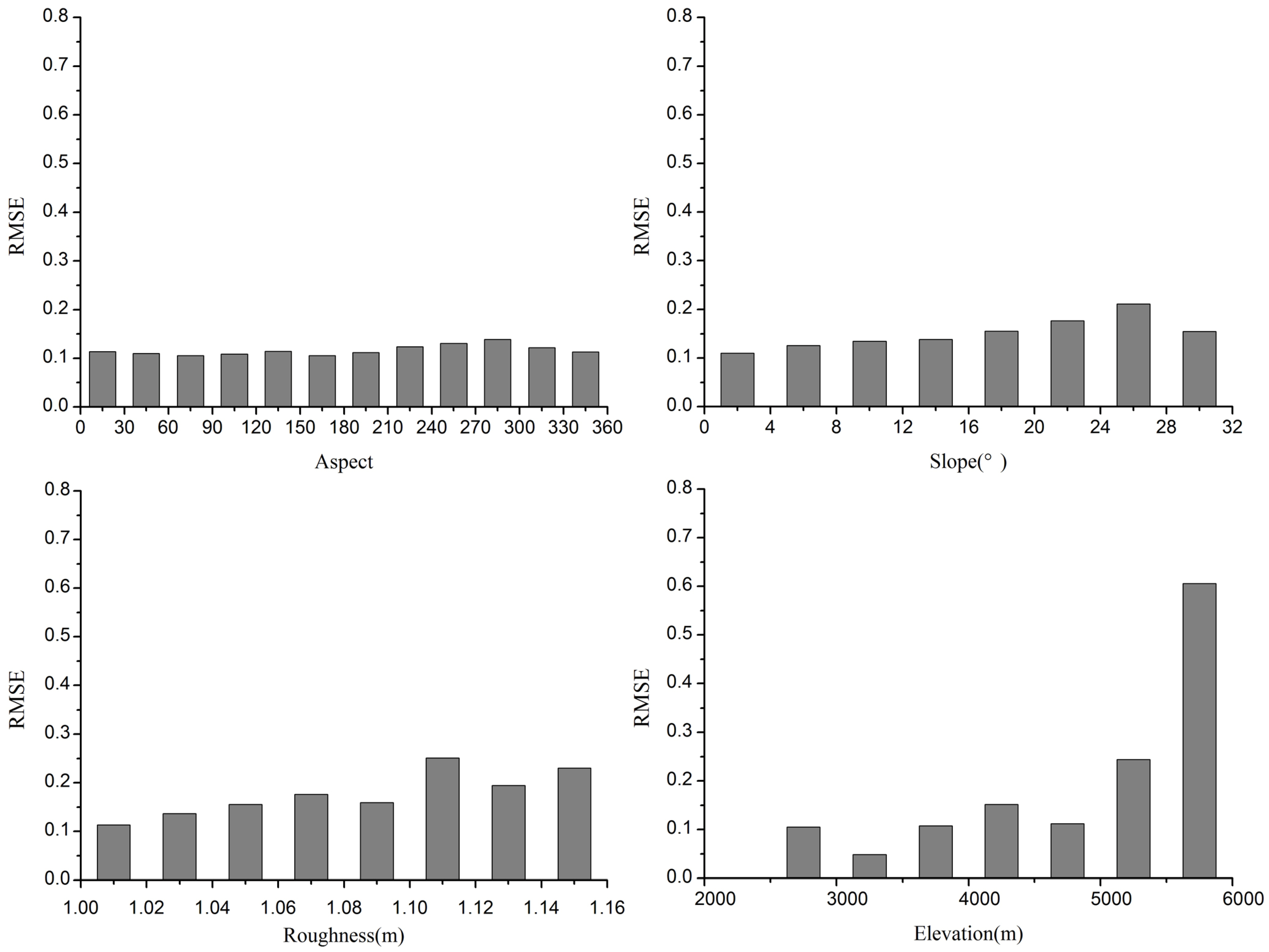
4.3. Error Analysis


5. Discussions
6. Conclusions
Acknowledgments
Author Contributions
Conflicts of Interest
References
- Robinson, D.A.; Frei, A. Seasonal variability of Northern Hemisphere snow extent using visible satellite data. Prof. Geogr. 2000, 52, 307–315. [Google Scholar] [CrossRef]
- Groisman, P.Y.; Karl, T.R.; Knight, R.W.; Stenchikov, G.L. Changes of snow cover, temperature, and radiative heat balance over the Northern Hemisphere. J. Clim. 1994, 7, 1633–1656. [Google Scholar] [CrossRef]
- Li, X.; Cheng, G.; Jin, H.; Kang, E.; Che, T.; Jin, R.; Wu, L.; Nan, Z.; Wang, J.; Shen, Y. Cryospheric change in China. Global Planet. Change 2008, 62, 210–218. [Google Scholar] [CrossRef]
- Xu, L.N.; Shi, J.C.; Zhang, H.G.; Wu, S.L. Fractional snow cover estimation in Tibetan Plateau using MODIS and ASTER. IEEE Int. Geosci. Remote Sens. Symp. 2005, 3, 1940–1942. [Google Scholar]
- Wang, J.; Li, H.; Hao, X.; Huang, X.; Hou, J.; Che, T.; Dai, L.; Liang, T.; Huang, C.; Li, H.; et al. Remote sensing for snow hydrology in China: Challenges and perspectives. J. Appl. Remote Sens. 2014. [Google Scholar] [CrossRef]
- Wang, C.H.; Wang, Z.L.; Cui, Y. Snow cover of China during the last 40 years: Spatial distribution and interannual variation. J. Glaciol. Geocryol. 2009, 31, 301–310. [Google Scholar]
- Dai, L.Y.; Che, T.; Wang, J.; Zhang, P. Snow depth and snow water equivalent estimation from AMSR-E data based on a priori snow characteristics in Xinjiang, China. Remote Sens. Environ. 2012, 127, 14–29. [Google Scholar] [CrossRef]
- Dai, L.Y.; Che, T. Spatiotemporal variability in snow cover from 1987 to 2011 in northern China. J. Appl. Remote Sens. 2014, 8, 084693. [Google Scholar] [CrossRef]
- Bai, Y.C.; Feng, X.Z. Introduction to some research work on snow remote sensing. Remote Sens. Technol. Appl. 1997, 12, 60–66. [Google Scholar]
- Danker, R.; De Jong, S.M. Monitoring snow-cover dynamics in Northern Fennoscandia with SPOT VEGETATION images. Int. J. Remote Sens. 2004, 25, 2933–2949. [Google Scholar] [CrossRef]
- Hartman, R.K.; Rost, A.A.; Anderson, D.M. Operational processing of multi-source snow data. In Proceedings of the 63rd Annual Western Snow Conference, Reno, NV, USA, April 1995.
- Xiao, X.; Zhang, Q.; Boles, S.; Rawlins, M.; Moore III, B. Mapping snow cover in the pan-Arctic zone, using multi-year (1998–2001) images from optical VEGETATION sensor. Int. J. Remote Sens. 2004, 25, 5731–5744. [Google Scholar] [CrossRef]
- Hall, D.K.; Riggs, G.A.; Salomonson, V.V.; DiGirolamo, N.E.; Bayr, K.J. MODIS snow-cover products. Remote Sens. Environ. 2002, 83, 181–194. [Google Scholar] [CrossRef]
- Che, T.; Li, X. Spatial distribution and temporal variation of snow water resources in China during 1993–2002. J. Glaciol. Geocryol. 2005, 27, 64–67. [Google Scholar]
- Che, T.; Li, X.; Jin, R.; Armstrong, R.L.; Zhang, T.J. Snow depth derived from passive microwave-remote sensing data in China. Ann. Glaciol. 2008, 49, 145–154. [Google Scholar] [CrossRef]
- Yu, H.; Feng, Q.S.; Zhang, X.T.; Zhang, X.T.; Huang, X.D.; Liang, T.G. An approach for monitoring snow depth based on AMSR-E data in the pastoral area of Northern Xinjiang. Acta Agrestia Sin. 2009, 18, 210–216. [Google Scholar]
- Liu, J.F.; Chen, R.S. Studying the spatiotemporal variation of snow-covered days over china based on combined use of MODIS snow-covered days and in situ observations. Theo. Appl. Climatol. 2011, 106, 355–363. [Google Scholar] [CrossRef]
- Hall, D.K.; Foster, J.L.; DiGirolamo, N.E.; Riggs, G.A. Snow cover, snowmelt timing and stream power in the Wind River Range, Wyoming. Geomorphology 2012, 137, 87–93. [Google Scholar] [CrossRef]
- Rodell, M.; Houser, P.R. Updating a land surface model with MODIS-derived snow cover. J. Hydrometeorol. 2004, 5, 1064–1075. [Google Scholar] [CrossRef]
- Platnick, S.; King, M.D.; Ackerman, S.A.; Menzel, W.P.; Baum, B.A.; Riédi, J.C.; Frey, R.A. The MODIS cloud products: Algorithms and examples from Terra. IEEE Trans. Geosci. Remote Sens. 2003, 41, 459–473. [Google Scholar] [CrossRef]
- Gafurov, A.; Bárdossy, A. Cloud removal methodology from MODIS snow cover product. Hydrol. Earth Syst. Sci. 2009, 13, 1361–1373. [Google Scholar] [CrossRef]
- Hall, D.K.; Riggs, G.A. Accuracy assessment of the MODIS snow products. Hydrol. Processes 2007, 21, 1534–1547. [Google Scholar] [CrossRef]
- Klein, A.G.; Barnett, A.C. Validation of daily MODIS snow cover maps of the Upper Rio Grande river basin for the 2000–2001 snow season. Remote Sens. Environ. 2003, 86, 162–176. [Google Scholar] [CrossRef]
- Maurer, E.P.; Rhoads, J.D.; Dubayah, R.O.; Dennis, P.L. Evaluation of the snow covered area data product from MODIS. Hydrol. Process. 2003, 17, 59–71. [Google Scholar] [CrossRef]
- Simic, A.; Fernandes, R.; Brown, R.; Romanov, P.; Park, W. Validation of vegetation, MODIS, and GOES+ SSM/I snow-cover products over Canada based on surface snow depth observations. Hydrol. Processes 2004, 18, 1089–1104. [Google Scholar] [CrossRef]
- Wang, X.; Xie, H.; Liang, T.G. Evaluation of MODIS snow cover and cloud mask and its application in northern Xinjiang, China. Remote Sens. Environ. 2008, 112, 1497–1513. [Google Scholar] [CrossRef]
- Huang, X.D.; Liang, T.G.; Zhang, X.T.; Guo, Z. Validation of MODIS snow cover products using Landsat and ground measurements during the 2001–2005 snow seasons over northern Xinjiang, China. Int. J. Remote Sens. 2011, 32, 133–152. [Google Scholar] [CrossRef]
- Cheng, Q.; Shen, H.; Zhang, L.; Yuan, Q.; Zeng, C. Cloud removal for remotely sensed images by similar pixel replacement guided with a spatio-temporal MRF model. ISPRS J. Photogramm. Remote Sens. 2014, 92, 54–68. [Google Scholar] [CrossRef]
- Li, X.H.; Shen, H.; Zhang, L.; Yuan, Q.; Yang, G. Recovering quantitative remote sensing products contaminated by thick clouds and shadows using multitemporal dictionary learning. IEEE Trans. Geosci. Remote Sens. 2014, 52, 7086–7098. [Google Scholar]
- Zeng, C.; Shen, H.F.; Zhang, L.P. Recovering missing pixels for Landsat ETM+ SLC-off imagery using multi-temporal regression analysis and a regularization method. Remote Sens. Environ. 2013, 131, 182–194. [Google Scholar] [CrossRef]
- Wang, X.; Xie, H. New methods for studying the spatiotemporal variation of snow cover based on combination products of MODIS Terra and Aqua. J. Hydrol. 2009, 371, 192–200. [Google Scholar] [CrossRef]
- Xie, H.; Liang, T.; Wang, X. Development and assessment of combined Terra and Aqua snow cover products in Colorado Plateau, USA and northern Xinjiang, China. J. Appl. Remote Sens. 2009. [Google Scholar] [CrossRef]
- Liang, T.G.; Huang, X.D.; Wu, C.X.; Liu, X.Y.; Li, W.L.; Guo, Z.G.; Ren, J.Z. An application of MODIS data to snow cover monitoring in a pastoral area: A case study in Northern Xinjiang, China. Remote Sens. Environ. 2008, 112, 1514–1526. [Google Scholar] [CrossRef]
- Parajka, J.; Blöschl, G. Spatio-temporal combination of MODIS images-potential for snow cover mapping. Water Resour. Res. 2008. [Google Scholar] [CrossRef]
- Hall, D.K.; Riggs, G.A.; Foster, J.L.; Kumar, S.V. Development and evaluation of a cloud-gap-filled MODIS daily snow-cover product. Remote Sens. Environ. 2010, 114, 496–503. [Google Scholar] [CrossRef]
- Gao, Y.; Xie, H.; Lu, N.; Yao, T.; Liang, T. Toward advanced daily cloud-free snow cover and snow water equivalent products from Terra-Aqua MODIS and Aqua AMSR-E measurements. J. Hydrol. 2010, 385, 23–35. [Google Scholar] [CrossRef]
- Liang, T.; Zhang, X.; Xie, H.; Wu, C.; Feng, Q.; Huang, X.; Chen, Q. Toward improved daily snow cover mapping with advanced combination of MODIS and AMSR-E measurements. Remote Sens. Environ. 2008, 112, 3750–3761. [Google Scholar] [CrossRef]
- Parajka, J.; Pepe, M.; Rampini, A.; Rossi, S.; Blöschl, G. A regional snow-line method for estimating snow cover from MODIS during cloud cover. J. Hydrol. 2010, 381, 203–212. [Google Scholar] [CrossRef]
- Huang, X.D.; Hao, X.H.; Feng, Q.S.; Wang, W.; Liang, T. A new MODIS daily cloud free snow cover mapping algorithm on the Tibetan Plateau. Sci. Cold Arid Reg. 2014, 6, 0116–0123. [Google Scholar]
- Wang, W.; Huang, X.D.; Deng, J.; Xie, H.; Liang, T. Spatio-temporal change of snow cover and its response to climate over the Tibetan Plateau based on an improved daily cloud-free snow cover product. Remote Sens. 2015, 7, 169–194. [Google Scholar] [CrossRef]
- Roesch, A.; Wild, M.; Gilgen, H.; Ohmura, A. A new snow cover fraction parameterization for the ECHAM4 GCM. Clim. Dyn. 2001, 17, 933–946. [Google Scholar] [CrossRef]
- Dobreva, I.D.; Klein, A.G. Fractional snow cover mapping through artificial neural network analysis of MODIS surface reflectance. Remote Sens. Environ. 2011, 115, 3355–3366. [Google Scholar] [CrossRef]
- Zhang, Y.; Huang, X.; Hao, X.; Wang, J.; Wang, W.; Liang, T. Fractional snow-cover mapping using an improved endmember extraction algorithm. J. Appl. Remote Sens. 2014. [Google Scholar] [CrossRef]
- Salomonson, V.V.; Appel, I. Estimating fractional snow cover from MODIS using the normalized difference snow index. Remote Sens. Environ. 2004, 89, 351–360. [Google Scholar] [CrossRef]
- Tang, Z.; Wang, J.; Li, H.; Yan, L. Spatiotemporal changes of snow cover over the Tibetan Plateau based on cloud-removed modereate resolution imaging spectroradiometer fractional snow cover product from 2001 to 2011. J. Appl. Remote Sens. 2012. [Google Scholar] [CrossRef]
- USGS EROS Data Center. MODIS Reprojection Tool User’s Manual; Release 4.1; 2011. Available online: https://lpdaac.usgs.gov/sites/default/files/public/mrt41_usermanual_032811.pdf (accessed on 13 February 2015).
- Friedl, M.A.; Damien, S.M.; Tan, B.; Schneider, A.; Ramankutty, N.; Sibley, A.; Huang, X. MODIS collection 5 global land cover: Algorithm refinements and characterization of new datasets. Remote Sens. Environ. 2010, 114, 168–182. [Google Scholar] [CrossRef]
- He, Y.; Bo, Y. A consistency analysis of MODIS MCD12Q1 and MERIS Globcover land cover datasets over China. In Proceedings of 19th International Conference on Geoinformatics, Shanghai, China, 24–26 June 2011.
- Huang, X.; Xie, H.; Liang, T.; Yi, D. Estimating vertical error of SRTM and map-based DEMs using ICESat altimetry data in the eastern Tibetan Plateau. Int. J. Remote Sens. 2011, 32, 5177–5196. [Google Scholar] [CrossRef]
- Dozier, J. Spectral signature of alpine snow cover from the Landsat Thematic Mapper. Remote Sens. Environ. 1989, 28, 9–22. [Google Scholar] [CrossRef]
- Carabajal, C.C.; Harding, D.J. ICESat validation of SRTM C-band digital elevation models. Geophys. Res. Lett. 2005. [Google Scholar] [CrossRef]
- Hao, X.H.; Wang, J.; Li, H.Y. Evaluation of the NDSI threshold value in mapping snow cover of MODIS. J. Glaciol. Geocryol. 2008, 30, 132–138. [Google Scholar]
© 2015 by the authors; licensee MDPI, Basel, Switzerland. This article is an open access article distributed under the terms and conditions of the Creative Commons Attribution license (http://creativecommons.org/licenses/by/4.0/).
Share and Cite
Deng, J.; Huang, X.; Feng, Q.; Ma, X.; Liang, T. Toward Improved Daily Cloud-Free Fractional Snow Cover Mapping with Multi-Source Remote Sensing Data in China. Remote Sens. 2015, 7, 6986-7006. https://doi.org/10.3390/rs70606986
Deng J, Huang X, Feng Q, Ma X, Liang T. Toward Improved Daily Cloud-Free Fractional Snow Cover Mapping with Multi-Source Remote Sensing Data in China. Remote Sensing. 2015; 7(6):6986-7006. https://doi.org/10.3390/rs70606986
Chicago/Turabian StyleDeng, Jie, Xiaodong Huang, Qisheng Feng, Xiaofang Ma, and Tiangang Liang. 2015. "Toward Improved Daily Cloud-Free Fractional Snow Cover Mapping with Multi-Source Remote Sensing Data in China" Remote Sensing 7, no. 6: 6986-7006. https://doi.org/10.3390/rs70606986