Urban Growth Simulation of Atakum (Samsun, Turkey) Using Cellular Automata-Markov Chain and Multi-Layer Perceptron-Markov Chain Models

Abstract

In this study, urban growth of the Atakum District in Samsun, Turkey, was simulated by Cellular Automata-Markov Chain (CA-MC) and Multi-layer Perceptron-Markov Chain (MLP-MC) hybrid models in a geographical information system (GIS) environment. Historical land use/land cover (LU/LC) data were extracted from 1989, 2000 and 2013 Landsat TM/ETM+/OLI images. Using the LU/LC data for the years 1989 and 2000, the urban growth for 2013 was simulated using the CA-MC and MLP-MC models. The simulation results were compared with the 2013 LU/LC data to assess the validity of the simulation. The MLP-MC method provided the best results according to the validation based on the kappa index of agreement. Based on this result, the urban growth for the year 2025 was simulated using MLP-MC. The simulation estimated an urban growth rate of 35.2% between 2013 and 2025, an increase in the area of artificial surfaces from 1681.9 ha to 2274.3 ha and the destruction of 511.7 ha of agricultural land and 4.4 ha of forest. The results of this study demonstrate that the urban growth models provide a better understanding of the current patterns and temporal dynamics and can predict future changes according to past and current dynamics. The results also show that simulations are most accurate when using a model that best conforms to the changes in the given study area.

1. Introduction

The urbanization process causes cities to rapidly grow and spread out over wide areas. Eventually, cities dominate the economic and social aspects of the surrounding urban and rural societies [1]. The urbanization process, generally perceived as modernization [2,3,4], is a problem in terms of unplanned and uncontrolled growth triggered by the rapid consumption of natural resources and by the rapid increase in populations, particularly in developing countries [1,5,6,7]. Although population increase due to migration is the leading growth factor in urban areas, many other factors, such as expectations of improved living standards as the result of economic development and higher incomes, the demand for larger living spaces, the loss of the charm of city centers due to transit and social outings, and the demand for secondary lodgings/summer houses, are responsible for the expansion of urban areas [8].

Along with urbanization, significant pressure is placed on natural resources. Agricultural lands, forests and wetlands are being destroyed [9], and forests are, in turn, being destroyed and converted to agricultural land [10]. Today, the combination of impervious surfaces, which are a product of the increasing number of structures and paved surfaces, and reduced agricultural land and forests has caused environmental problems in cities, such as environmental pollution, floods and landslides [11,12,13,14]. Thus, the importance of urban analysis has gradually increased. In the broadest sense, urban analysis is defined as the solution to urban problems through revealing the current conditions of a city [15,16]; the method requires interdisciplinary research. Issues such as city ecology, socio-economics, demography, urban heat-island effects, assessment of land use/land cover (LU/LC), and the simulation of urban growth can all be addressed within the scope of urban analysis [16,17]. In particular, simulation models are essential in the prediction of future urban changes and in planning studies [18,19].

While the analyses and studies of the past to the present rely on evidence, model studies of the future rely on predictions. However, future predictions are also directly related to changes observed from the past to the present [16]. Both the analysis of current conditions and model studies are spatial tools due to the nature of the issues relevant to a city; thus, the solutions also require spatial studies. For this reason, remote sensing and geographical information systems (GIS) are widely used in the determination of past and present LU/LC to understand city patterns, detect changes, and monitor or model processes [16,20,21,22,23]. Within this scope, various urban studies on patterns, processes, causes, results, simulations and countermeasures have become increasingly important [16].

In urban studies, the phrases “urban growth”, “urban expansion” and “urban sprawl” are generally synonymous and are used to define the increase in urban areas. However, Bhatta (2010) specified that these phrases are different and that urban expansion and urban sprawl are forms of urban growth. Expansion is defined as the transformation of non-urban areas surrounding the urban areas to urban use; sprawl is defined as the transformation of areas far from the current urban area to urban use. According to Bhatta (2010), urban growth should be analyzed both as a land use pattern of a specific spatial configuration in an area at a specific time and as the processes that reflect the changes in the spatial structure of the city over time. Urban growth is a static phenomenon if it is considered a pattern, while it is a dynamic phenomenon if it is considered a process [16]. The analysis of urban growth as a pattern and process improves our understanding of the changes in city patterns over time by revealing the dynamic processes of the city and by making predictions [16,24]. In urban analysis, information regarding the rate of urban growth, the spatial configuration of the growth, the discrepancies between observed and predicted growth, spatial or temporal disparities in the growth and uncontrolled growth can be determined. With this information, possible risks may be prevented by making predictions [16]. Within this scope, the direction of planning by identifying the limits of urbanization and by developing essential strategies for environmental sustainability can be ensured [22].

The quality of predicted changes depend on the accuracy of the analysis of the past and present conditions, the data quality, and the model used for the predictions [25]. In recent years, many models have been adapted to simulate LU/LC changes and urban growth. Markov chain (MC) models, regression models, cellular automata (CA) models, agent-based models, artificial neural networks (ANNs), and optimization models are among the widely used models [20,25,26,27,28,29]. Each model has advantages and disadvantages [27,30]. Thus, various hybrid models have also been adapted to simulate urban growth [19,22,25,31,32,33,34,35,36]. Determining which hybrid model provides the best results is difficult because each study reaches unique conclusions. Thus, in general, instead of specifying a single method, the method that provides the best results for the study area should be used. For this reason, studies based on the principle of comparing models and running simulations with the method that provides the best results for the study area are becoming more popular [37,38,39,40,41].

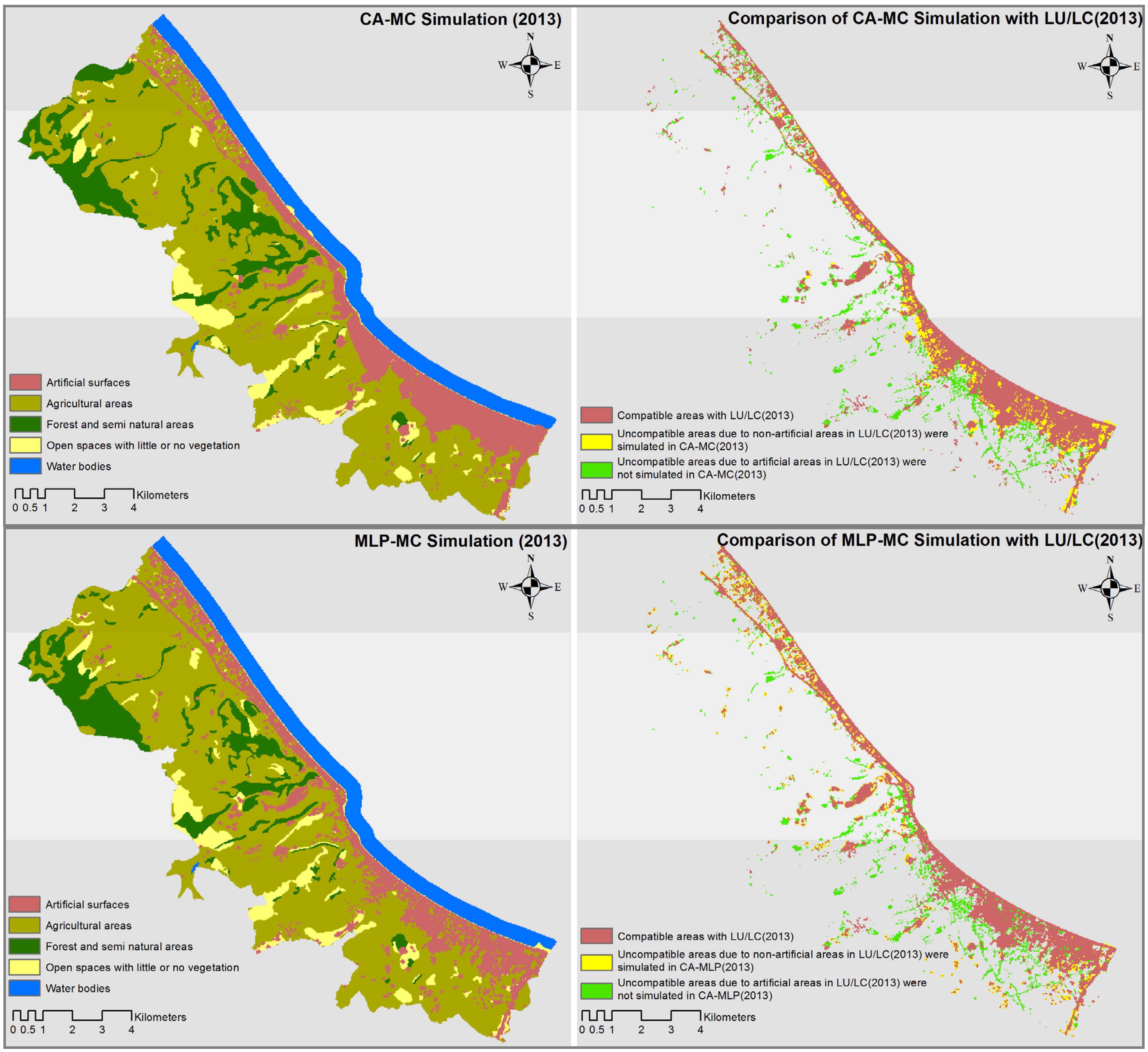
In this study, Cellular Automata-Markov Chain (CA-MC) and Multi-layer Perceptron-Markov Chain (MLP-MC) hybrid models were used to simulate LU/LC changes and urban growth in the Atakum District (Samsun, Turkey), where the population growth is rapid, despite the general stability of the population of Samsun Province. The objectives of this study are to: (i) understand the pattern of urban growth, (ii) identify the possible growth scenario via future simulations, and (iii) determine the method that provides the best results in the study area. For this purpose, the urban growth for the year 2013 was simulated by the CA-MC and MLP-MC models based on the LU/LC data from 1989 and 2000. The results of the simulations were compared with the LU/LC data from 2013. The MLP-MC model provided the best results in the study area. A 2025 scenario was simulated by MLP-MC. The simulation for 2025 was compared with the LU/LC data from 2013, and the transition directions, quantities and spatial distributions of possible changes in 2013–2025 were determined.

2. Study Area: Atakum

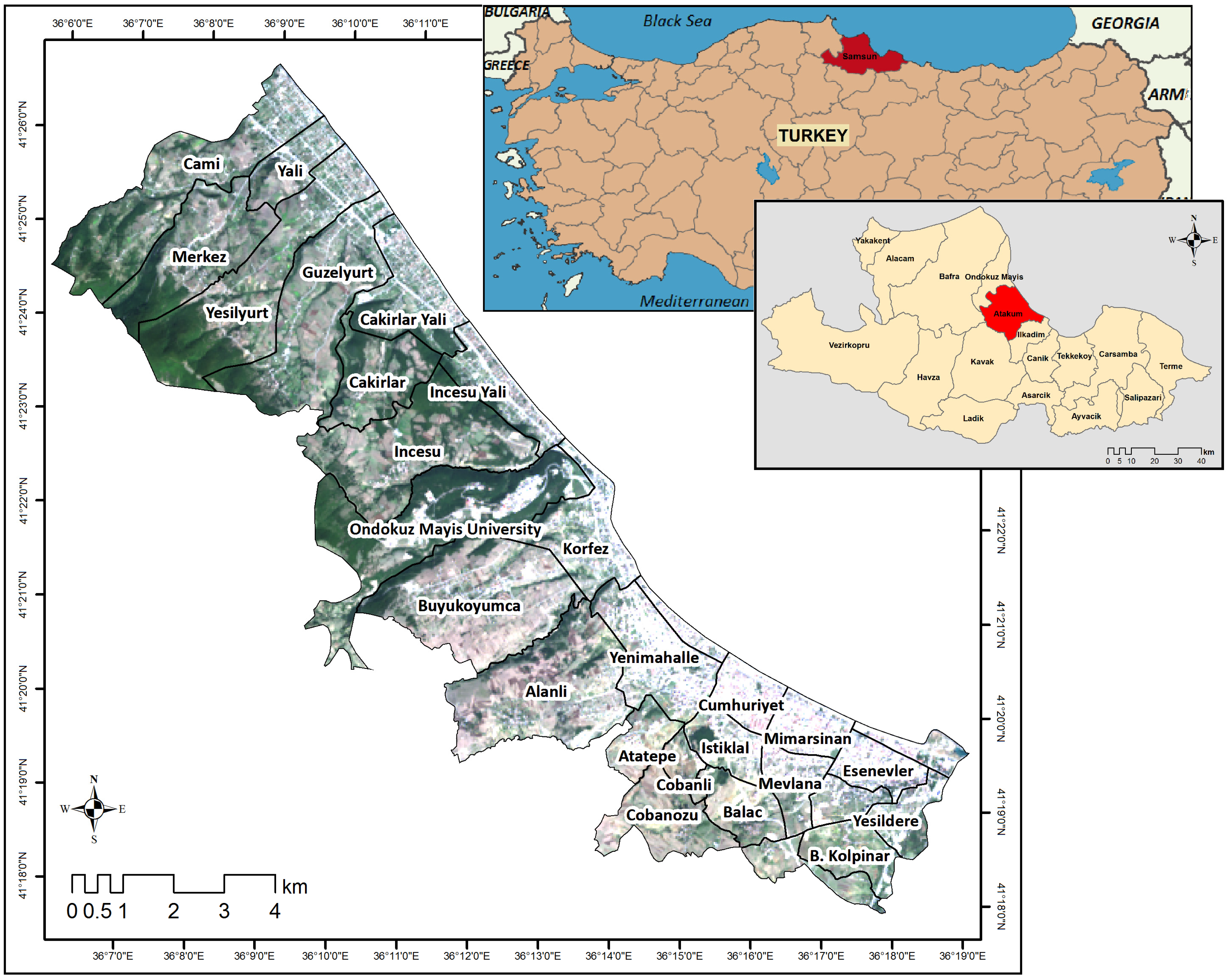
Atakum (Figure 1) is a district in Samsun Province, Turkey, and is located between 35°58ʹ45ʺ–36°19ʹ00ʺE and 41°13ʹ30ʺ–41°26ʹ45ʺN. The area was referred to as Matasyon until 1994, at which time it became a county municipality with the name Atakum. In accordance with Law No. 5747, which was enforced after publication in the Official Gazette No. 26824 on 22 March 2008, the counties of Atakent, Kurupelit, Altinkum, Catalcam and Taflan were merged with Atakum. Atakum gained the status of a district on 1 July 2008. The total surface area of Atakum is approximately 354 km². Atakum is bordered by the Ilkadim District to the east, the Ondokuz Mayis District to the west, the Black Sea to the north, and the Kavak and Bafra Districts to the south. Atakum extends 20 km westward along the sea coast from the Kurtun River [42]. The district comprises four morphological units: coastal plains, sloping lands, low plateaus and mountainous areas. The coastal plains are fertile lands that formed by the alluvium in the Kurtun River to the east and by the Kizilirmak River to the west, but nearly all of the coastal plains have been used for settlements. In Atakum, most settlements are constructed on the coastal plains. Intense settlement is also observed on the sloping areas between the coastal plains and low plateaus. The annual average temperature of Atakum, which experiences a temperate climate, is 14.4 °C, according to 2011 data. The average temperature in February, the coldest month in the district, is 6.9 °C. The average temperature in August, the hottest month, is 23.5 °C. The annual total precipitation is 691 kg/m². The precipitation in Atakum is among the lowest in the Black Sea region [43].

Figure 1. Location of the study area. The 29 sectors of the study area are shown on a true-color composite of Landsat-8 OLI 2013 imagery.

Figure 1. Location of the study area. The 29 sectors of the study area are shown on a true-color composite of Landsat-8 OLI 2013 imagery.

The economy of Atakum, which has generally relied on agriculture and stockbreeding since the 1980s, is now dominated by the service sector. The sea is generally clean and suitable for swimming, and numerous summer houses, accommodation facilities for tourism purposes, entertainment venues and restaurants have been constructed along the coastline. Atakum features the highest population increase within Samsun Province [42]. Because the borders of the district were finalized in 2008 and because the population data prior to that year did not conform to the borders, the population information prior to 2008 is misleading. The population of the district was 107,953 in 2008 and 158,031 in 2014 [44]. The district has an annual average growth rate of approximately 63.5‰, and it experiences significant migrant populations from other districts in Samsun and other provinces. Although the annual natural population increase in the district is approximately 1500, the total population increase including migration is approximately 8500. The average annual population increase over 2008–2014 was 4.8‰ in Samsun Province and 13.8‰ in Turkey; thus, Atakum experienced a population increase rate much higher than the averages for Turkey and Samsun. Moreover, although the total population of Samsun decreased by 0.7‰ over 2010–2011 and no change in the population was observed over 2011–2012, increases of 58.4‰ and 61.8‰ were observed in Atakum in 2010–2011 and 2011–2012, respectively. In the literature, this high rate of migration to Atakum is attributed to the presence of one of the largest and most important universities in the Black Sea region, the available transportation, the appeal of the coast and beaches, and the low crime rates [43].

This study focuses on the portion of Atakum with the greatest population increase, a high urbanization potential and urban development. The 91 km² area consists of 29 sectors and contains 94.7% of Atakum’s population (Figure 1).

3. Data and Methodology

To model the urban growth of Atakum, this study was conducted in three phases. The first phase involved the collection of data that covered the study area and the preparation of the LU/LC layers for several years. Because the topographic data of the study area was limited, and because of the difficulties in obtaining past data, it was decided to use satellite images. Landsat images were selected from among the various levels of spatial, spectral, radiometric and temporal resolution satellite images because of their long-term availability [45], cost-effectiveness, and timeliness [46]. The LU/LC layers were generated by using Landsat-4 TM satellite image from 2 August 1989, Landsat-7 ETM+ satellite image from 13 June 2000, and Landsat-8 OLI satellite image from 13 September 2013 (path/row: 175/31). All images were obtained from the U.S. 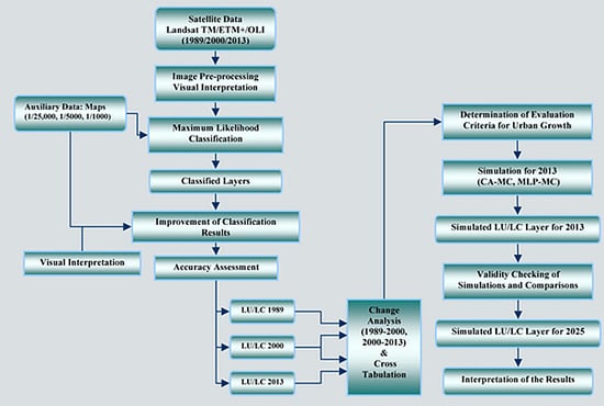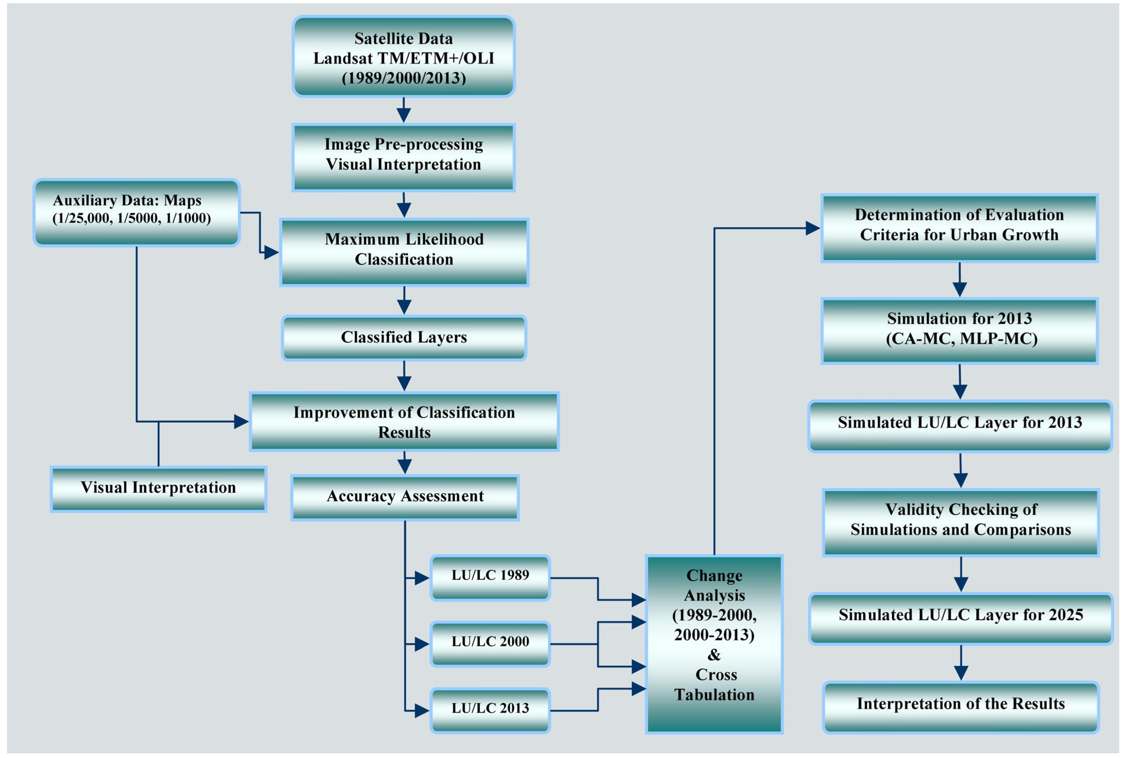Geological Survey [47,48]. In the second phase, the LU/LC changes were analyzed. In the final phase, the factors that affect urban growth were determined, and the urban growth based on past changes and the factors was simulated. As auxiliary data, 1/25,000-, 1/5000- and 1/1000-scale maps that cover various areas in various years were used for processing and classifying the images and for preparing the factor layers. To process the satellite images and to simulate the urban growth, the IDRISI 17.0 Selva software package (Clark Labs, Clark University, Worcester, MA, USA) was used. ARIS Grid Editor (ARIS B.V., Utrecht, The Netherlands), operating in ArcGIS 10.0 software (Esri, Redlands, CA, USA), was used to enhance the classified images. To develop a model of urban growth, the IDRISI CA_Markov and The Land Change Modeler (LCM) modules were used. The primary operations of the methodology are shown in Figure 2.

3.1. Preprocessing of Satellite Images and Classification

The Landsat data were geometrically corrected and registered to a common UTM projection. For this purpose, a 2013 Landsat OLI image was first geo-referenced using 1/25,000-scale topographic maps and 1/5000- and 1/1000-scale base maps. Then, the images from 1989 and 2000 were image-to-image registered using the 2013 images. The root mean square error (RMSE) was carefully kept below 0.5 pixels. Following the geo-referencing operation, the images were classified with the maximum likelihood method (all bands were used except for the thermal bands due to the spatial resolution). The maximum likelihood procedure is the most widely used classifier of remotely sensed imagery and is based on Bayesian probability theory. Using the information from a set of training sites, the method uses the mean and variance/covariance data of the signatures to predict the probability that a pixel belongs to each class [49]. In the classification, the categories of the Coordination of Information on the Environment (CORINE) classification system [50] were used (Table 1). For each class, 100 training samples were selected from the maps of the classification area.

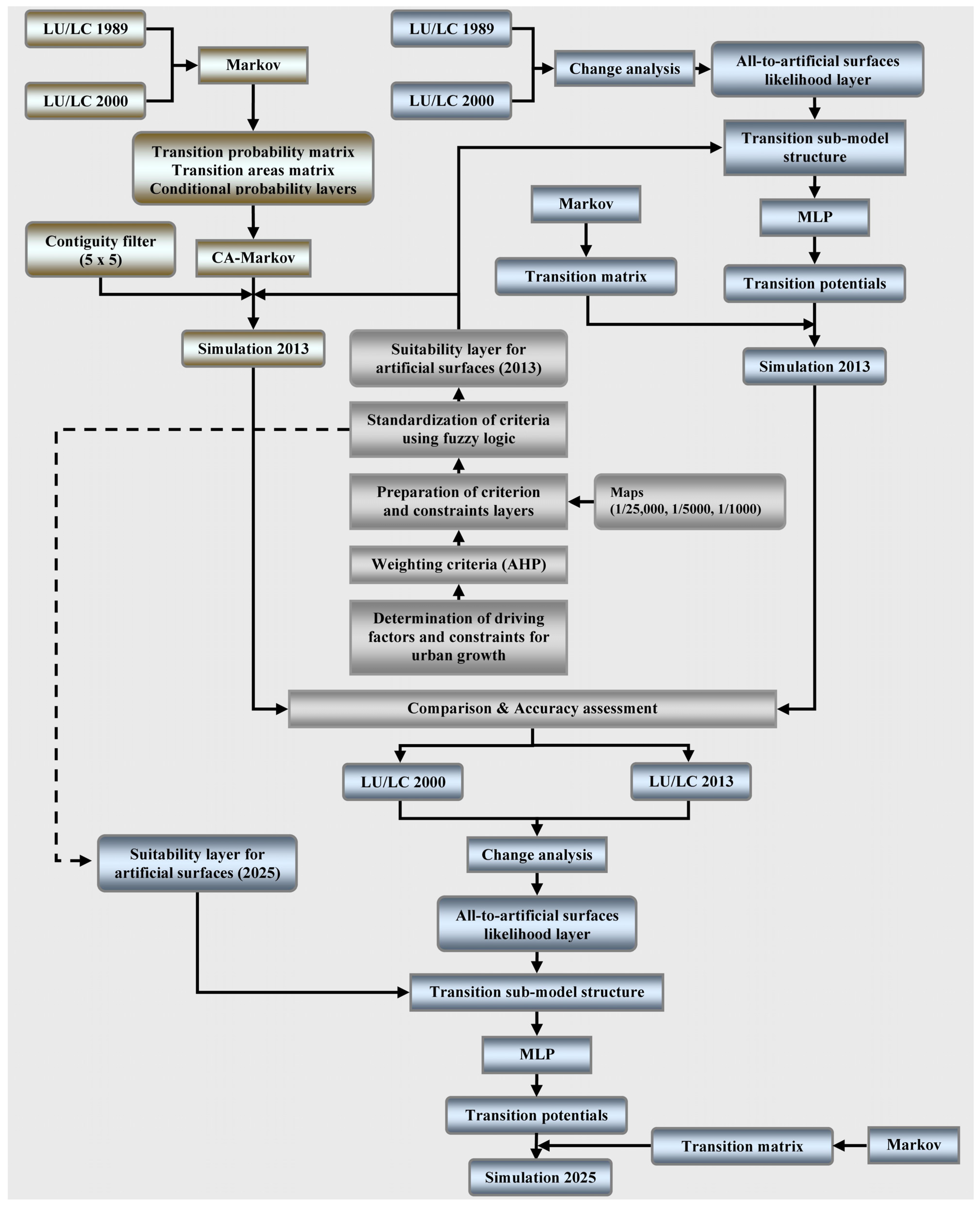
Figure 2. Workflow showing the main operations in the study. In the first phase, the Landsat images were classified, and the LU/LC layers were prepared. In the second phase, the changes that occurred in 1989–2000 and 2000–2013 were identified. In the third phase, the urban growth was simulated for 2013 with the CA-MC and MLP-MC methods. The simulation for 2025 was obtained by determining the method that provided the best results in the study area through a comparison of the results with the LU/LC data from 2013.

Figure 2. Workflow showing the main operations in the study. In the first phase, the Landsat images were classified, and the LU/LC layers were prepared. In the second phase, the changes that occurred in 1989–2000 and 2000–2013 were identified. In the third phase, the urban growth was simulated for 2013 with the CA-MC and MLP-MC methods. The simulation for 2025 was obtained by determining the method that provided the best results in the study area through a comparison of the results with the LU/LC data from 2013.

Table 1. LU/LC classes used in the study.

Class	Content (Features in the Study Area)
Artificial surfaces	Residential areas, commercial and industrial areas, roads and other construction sites
Agricultural areas	Active farmland
Forest and semi-natural areas	Forest, grove, active/passive green spaces
Open spaces with little or no vegetation	Bare soil, beach, sparsely vegetated areas, sand, gravel and stone quarries
Water bodies	Sea, dam reservoir, river

Table 1. LU/LC classes used in the study.

Class	Content (Features in the Study Area)
Artificial surfaces	Residential areas, commercial and industrial areas, roads and other construction sites
Agricultural areas	Active farmland
Forest and semi-natural areas	Forest, grove, active/passive green spaces
Open spaces with little or no vegetation	Bare soil, beach, sparsely vegetated areas, sand, gravel and stone quarries
Water bodies	Sea, dam reservoir, river

Because the pixel size of the images used in the analyses is 30 m, the classified LU/LC layers have a 30 m pixel size. The classified image was visually examined using the various band combinations and maps of the area, and the results were improved through editing with ARIS Grid Editor. The accuracy assessment of the obtained results is an estimate of the quality and usability of the products, and it is based on the principle of comparing each class in the classified image with the ground-truth test data. Therefore, a confusion matrix was developed. The accuracy assessment was composed of the producer accuracy, user accuracy, overall accuracy and kappa value [51]. If the kappa value is greater than 0.8, then strong to perfect agreement exists; if the value is between 0.6 and 0.8, then strong to substantial agreement exists; if the value is between 0.4 and 0.6, then moderate agreement exists; and if the value is less than 0.4, then weak agreement exists [52]. In this study, the confusion matrix was composed of 250 test points obtained for each class based on maps of the area. The accuracy of the LU/LC layers were analyzed for 1989, 2000 and 2013.

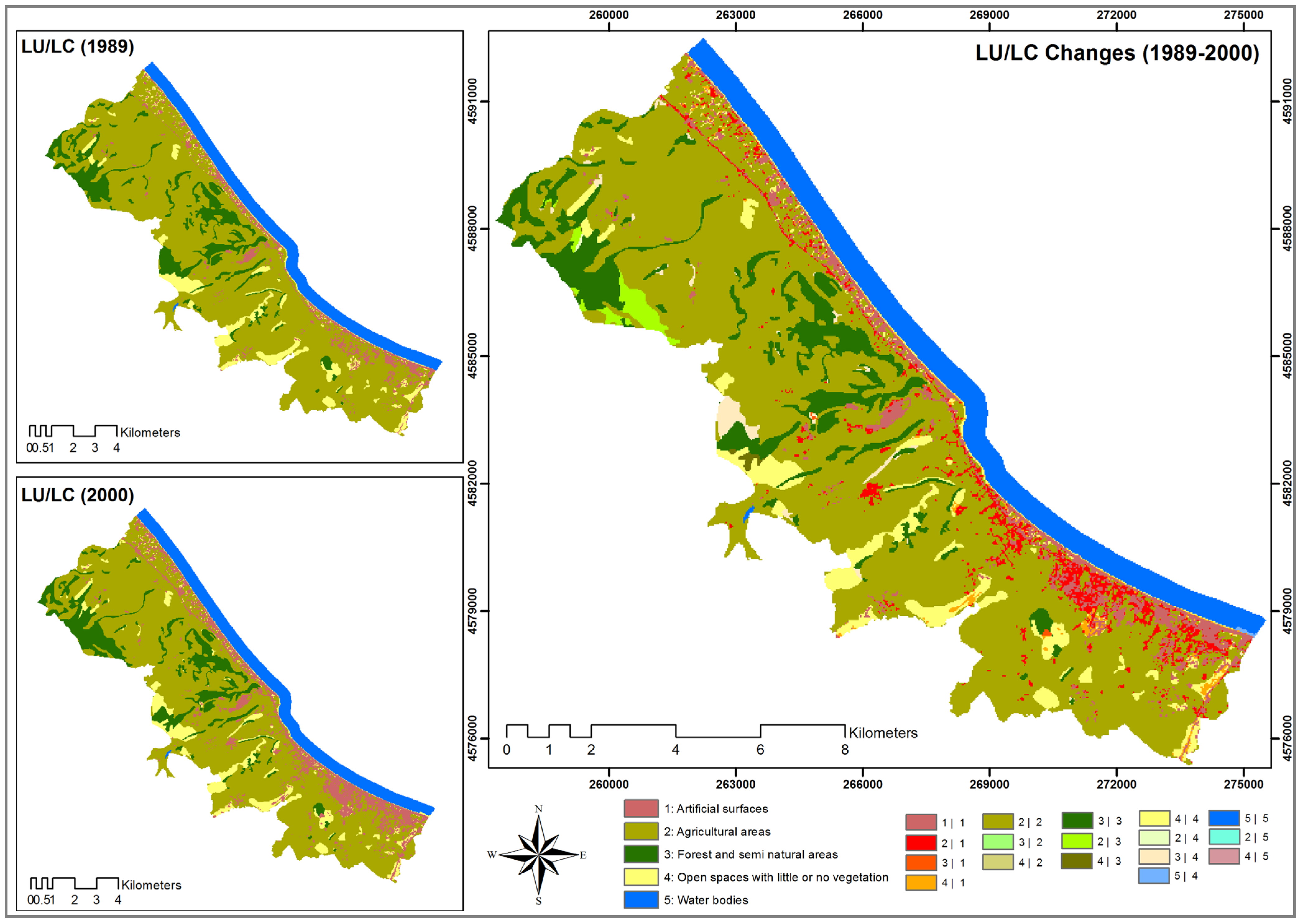
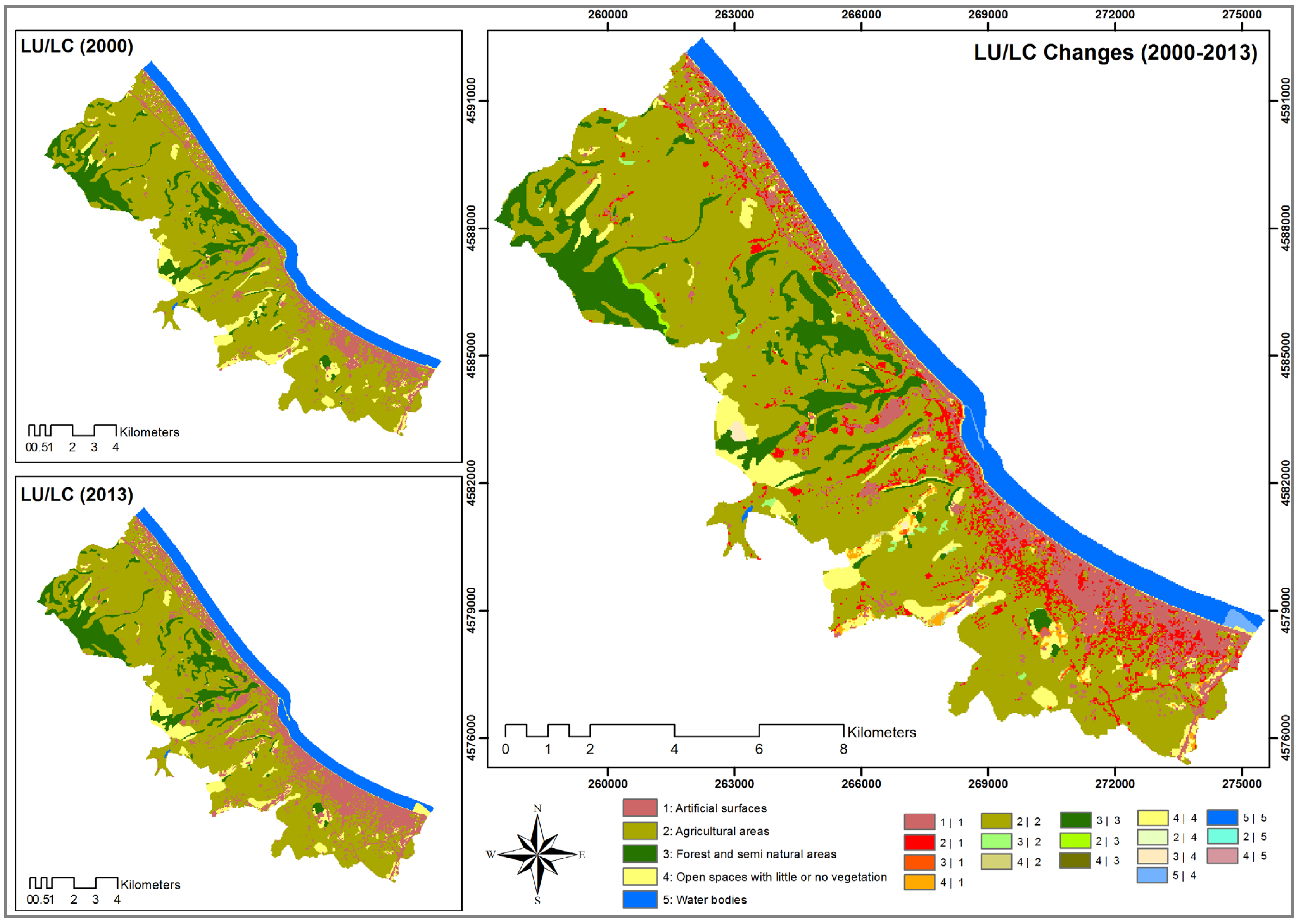
3.2. Change Analysis

In urban areas, the LU/LC system is subjected to intense pressure by humans; thus, urban areas have complex spatio-temporal change dynamics [39]. These changes significantly affect natural resources, the environment, socio-economic factors, etc. Identifying the changes and their causes would help determine possible future changes, decision-support phases and the composition of various LU/LC change scenarios [16]. Change analysis is based on the historical changes from time t₁ to t₂ [49]. Based on the analysis of LU/LC changes, the transition from one class to another within a specific period is determined, thereby revealing the interactions between the classes [39]. In this study, cross-tabulation analysis [49,53] was applied to determine the LU/LC changes over 1989–2000 and 2000–2013. Based on this analysis, the areas that changed from one class to another at specific periods can be determined spatially and quantitatively [25]. The cross-tabulation table shows the frequencies of changed or unchanged classes [49].

3.3. Simulation

In the study, the CA-MC and MLP-MC hybrid models were used to simulate the LU/LC changes and urban growth. The simulation results obtained for 2013 were compared with the LU/LC data for 2013. The MLP-MC model provided the best results in the study area; thus, the simulation for 2025 was performed using MLP-MC, and possible changes were determined. The workflow of the simulation is shown in Figure 3.

3.3.1. CA-MC

The CA method is a system used to divide facts or issues by cell and to determine the future status of each cell based on neighboring cells [54,55]. CA has four elements: X, S, N and f. X is the group of cells composing the space of the study area; S is the non-empty finite group of automata statuses, where each cell can have only one status at a specific time; N defines the contiguity for a specific cell; and f (transition function) consists of a set of rules that determines the future status of a cell based on the current status of the cell and its neighboring cells [20].

Figure 3. Workflow of the simulation of urban growth. In the first phase, the urban growth simulation was performed by the CA-MC and MLP-MC methods for the year 2013. The same data were used in both simulations, and the areas with changes were calculated with the MC. Based on the validity assessment of the simulation results, the simulation for 2025 was run using MLP-MC, which provided the best results in the study area.

Figure 3. Workflow of the simulation of urban growth. In the first phase, the urban growth simulation was performed by the CA-MC and MLP-MC methods for the year 2013. The same data were used in both simulations, and the areas with changes were calculated with the MC. Based on the validity assessment of the simulation results, the simulation for 2025 was run using MLP-MC, which provided the best results in the study area.

An MC is a stochastic process that defines the probability that one status will transform into another status. The key identifier in the MC is the “transition probability matrix”, and a future status is predicted through the analysis of past statuses. The MC model is defined as the group of statuses, and a process starts at one status and moves consecutively from one status to another [19,53].

One of the main spatial elements that underlies the numerous dynamics is contiguity. When an area is close to areas in another class, the area exhibits a high tendency to transform into that class. This tendency is referred to as the expansion phenomenon [49]. Although the MC is a practical method for modeling changes and determining future trends, it cannot be used alone in spatial simulation studies because it does not consider the effects of neighboring cells and does not provide the opportunity to spatially model the predicted change. In other words, the MC method lacks a spatial component [19,56]. In the CA method, only the cells surrounding a cell of interest are considered in the estimation of the future status of the cell. By integrating these two approaches, one can assess both the spatial relations and past statuses in the simulation of future statuses. In a hybrid CA-MC model, the transition probabilities are calculated using LU/LC layers that belong to different periods (t₁: Earlier date and t₂: Later date). The temporal dynamics between LU/LC classes are determined using transition probabilities. Spatial dynamics are determined with local rules, in which CA assesses the contiguity configuration and transition probabilities [56]. In the CA-MC method, the base LU/LC layer (belonging to t₂), the transition areas for future projection dates produced by the MC (using LU/LC layers of t₁ and t₂), and the transition-potential layers for each LU/LC class are used. The transition-potential layers specify the degree to which each cell is suitable for each of the LU/LC types. In the CA-MC method, the allocation of pixels (spatially projected) for each LU/LC continues iteratively until the areas predicted by the MC analysis (transition areas) are met [49]. The number of iterations is equal to the number of years from the base date to the projection date. A contiguity filter is used to change the status of each cell based on the previous statuses of the cells and on the statuses of contiguous cells. In this study, the following 5 × 5 contiguity filter (Equation (1)) was applied to transition-potential layers composed of LU/LC types. The filter used in the study has been used extensively to simulate settlements; however, the filter is able to change, depending on the purpose of the study and on the selection of the analyst [53,56,57].

$$\text{Contiguity filter }(5\text{x}5)=\left[\begin{array}{ccccc}0& 0& 1& 0& 0\\ 0& 1& 1& 1& 0\\ 1& 1& 1& 1& 1\\ 0& 1& 1& 1& 0\\ 0& 0& 1& 0& 0\end{array}\right]$$

(1)

3.3.2. MLP-MC

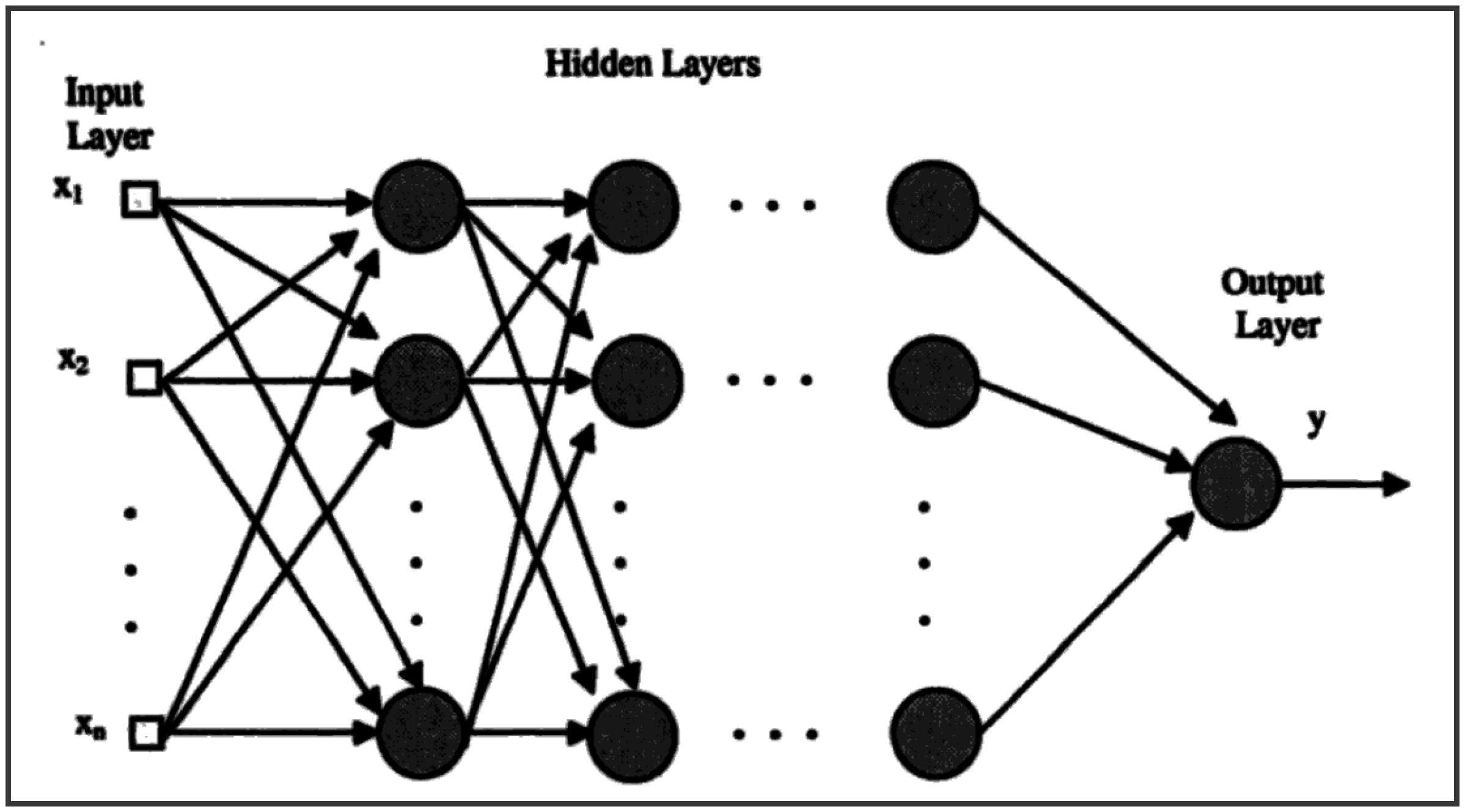
In this approach, transitions are modeled using a MLP neural network. The MLP method is the most common type of neural network [58], and it is often called a “back-propagation” network because of its training rules. The MLP consists of an input layer, one or more hidden layers and an output layer [59,60] as shown in Figure 4. Multi-layer perceptrons are often fully connected, i.e., every neuron in each layer is connected to other neurons in neighboring layers [61].

Figure 4. The MLP architecture with the organization of layers (Reused from Ref. [60], Figure 8.2 with permission of Springer Science+Business Media).

Figure 4. The MLP architecture with the organization of layers (Reused from Ref. [60], Figure 8.2 with permission of Springer Science+Business Media).

Sub-models are developed to determine the transition potential in the MLP-MC method. Each sub-model is defined for relevant variables. Static and dynamic variables can be added to the model. Static variables do not change with time. Dynamic variables can change during the simulation, and they are also computed while performing a prediction. After calculating the potential transition layers with MLP, a prediction is made. The MC analysis is used in the simulation phase [49,62].

Only major transitions are included in the sub-models to obtain superior results in the MLP-MC method [53]. Because determining urban growth is the main purpose, the transition to artificial surfaces from other classes [39] is addressed as a sub-model.

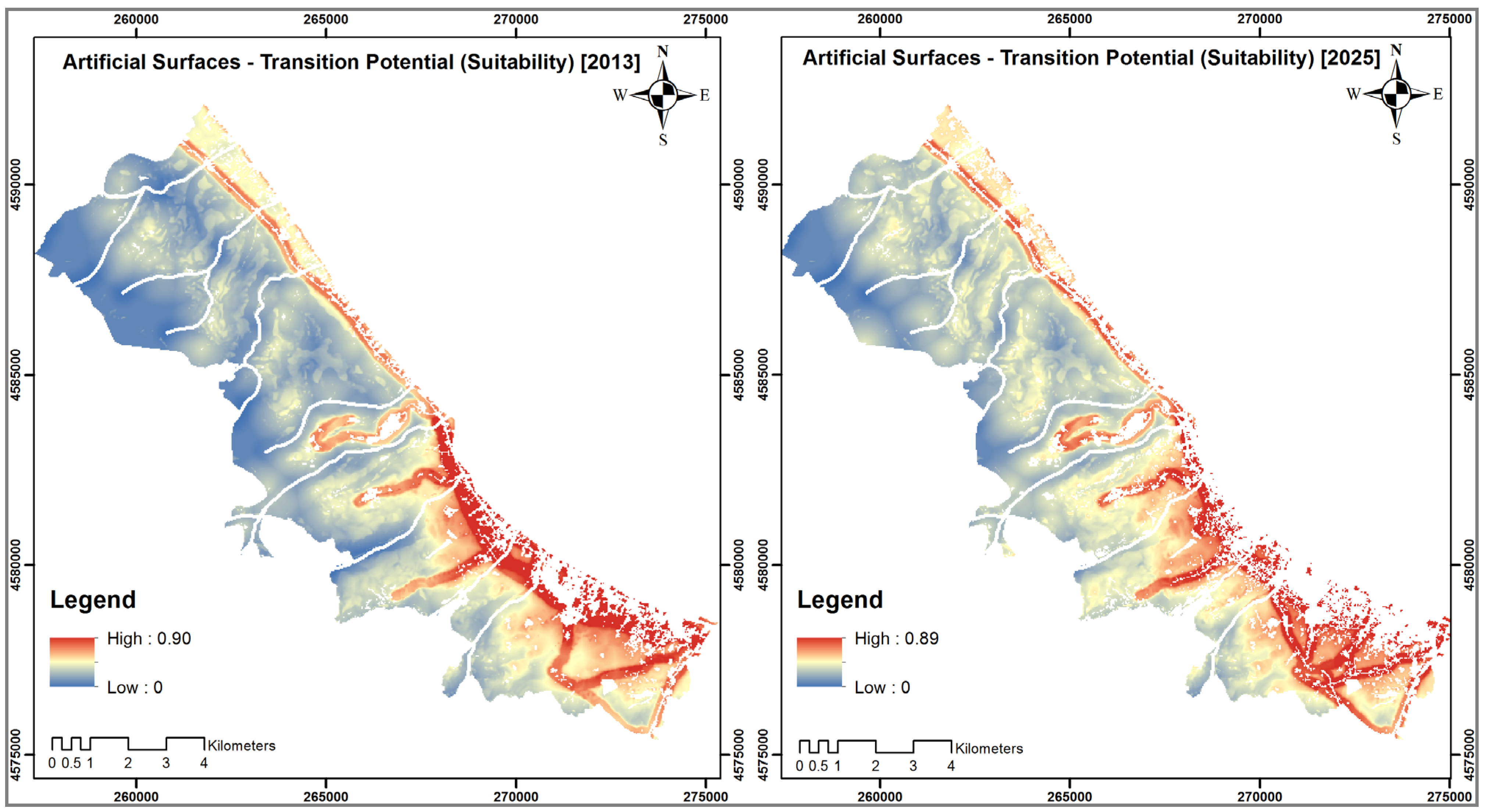
3.3.3. Determination of Transition Potential

A transition potential image-layer indicates the relative likelihood of transition of one LU/LC class to another for each pixel [63]. The transition potentials must be determined to model the changes in both the CA-MC and MLP-MC simulations. These layers are generally produced through the calibration step of the simulation. CA-MC generally uses suitability layers which are produced by multi-criteria evaluation (MCE) as transition potential [63] and in MLP-MC, a collection of transition potential layers is organized within an empirically evaluated transition sub-model that has the same underlying driver variables [49].

In this study, the artificial surfaces-suitability layer was prepared using the analytical hierarchy process (AHP), which is one of the most extensively used MCE methods, to determine the transition potential of the artificial surfaces class. Conditional probability layers obtained by the MC process for the agricultural areas, forests, semi-natural areas, open spaces with little or no vegetation and water bodies were used as transition potential layers in the CA-MC method.

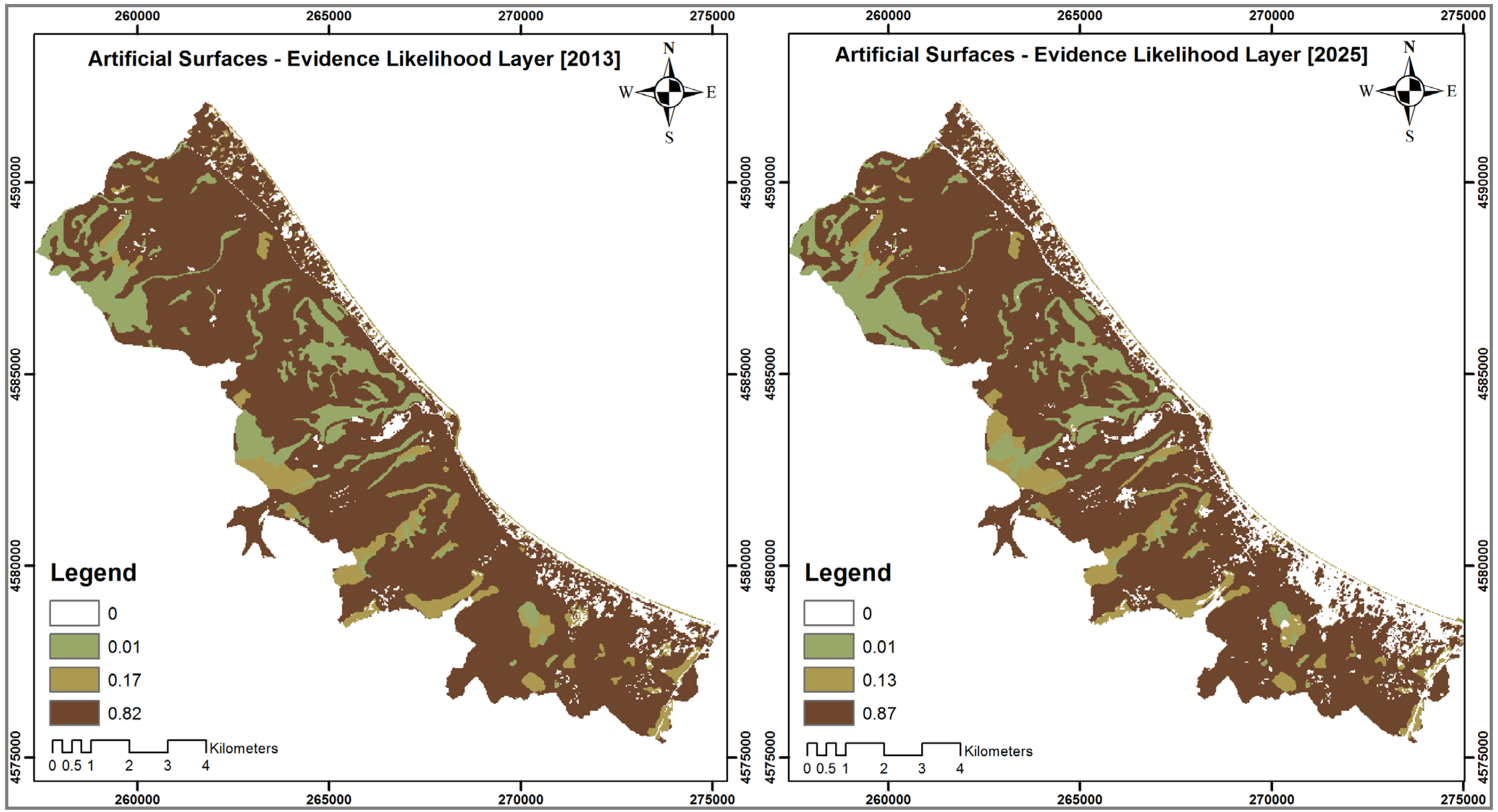
Additionally, in the MLP-MC method, the variables of the sub-model were determined as an artificial surfaces-suitability layer and evidence-likelihood layer as in the study by Baysal (2013) [39]. The evidence-likelihood layer is created by determining the relative frequency with which different LU/LC categories occurred within the areas that transitioned between times t₁ and t₂ [53]. In this study, the evidence-likelihood layer was based on changes from other classes to the artificial surfaces class (“all to artificial surfaces”).

Artificial surfaces-Suitability Layer

In the preparation of the suitability layer for artificial surfaces, the factors that cause urban growth in the study area were determined. Urban growth is generally the result of complex interactions between many factors. Thus, a factor set that is universally defined in all studies for all areas is difficult to generate [25,64]. However, based on literature surveys, similar factors were used in other studies and it was decided to use the factors in Table 2 in this study [25,39,64]. In addition, unsuitable areas for urbanization were identified as constraints, as shown in Table 2. The existing building areas, water-covered areas and the locations not allowed for urban development by zoning regulations of the Atakum District local administration and the Turkish Zoning Law were evaluated as the areas not suitable for urban growth. The constraint areas were masked to exclude them from the urban growth simulation.

Table 2. Definition of driving factors of LU/LC changes and constraints.

Factors	Constraint (Areas not Suitable for Urban Growth)
Distance to main urban centers	Areas not geologically suitable for settlement
Distance to tram system	20 m from riverside (flood risk boundaries of rivers)
Distance to major roads	50 m from sea coastline
Distance to existing built-up surfaces	Areas covered with water
Distance to sea coast	Current artificial surfaces
Slopes (percent)
Distance to rivers
Because major roads and existing built-up surfaces vary by year, the distance to existing built-up surfaces and the distance to major roads were calculated in both the 2013 simulation and 2025 simulation. The constraints layer (due to artificial surface changes) for the 2013 and 2025 simulations were also arranged. The situation in 2000 was taken into account for the 2013 simulation, and the situation in 2013 was taken into account for the 2025 simulation.

Table 2. Definition of driving factors of LU/LC changes and constraints.

Factors	Constraint (Areas not Suitable for Urban Growth)
Distance to main urban centers	Areas not geologically suitable for settlement
Distance to tram system	20 m from riverside (flood risk boundaries of rivers)
Distance to major roads	50 m from sea coastline
Distance to existing built-up surfaces	Areas covered with water
Distance to sea coast	Current artificial surfaces
Slopes (percent)
Distance to rivers
Because major roads and existing built-up surfaces vary by year, the distance to existing built-up surfaces and the distance to major roads were calculated in both the 2013 simulation and 2025 simulation. The constraints layer (due to artificial surface changes) for the 2013 and 2025 simulations were also arranged. The situation in 2000 was taken into account for the 2013 simulation, and the situation in 2013 was taken into account for the 2025 simulation.

The AHP method was used to create the artificial surfaces-suitability layer for 2013 and 2025. The AHP method was developed by Saaty (1980) [65]. The AHP is a theory of measurement that uses pairwise comparisons and that relies on the judgments of experts to derive priority scales [66,67,68]. Pairwise comparisons are determined by a scale with values from 1 to 9 [65,69]. In the AHP, the factor (criterion) weights are determined using pairwise comparison. The AHP also allows decision alternatives to be prioritized using pairwise comparison [70]. However, it is difficult to perform pairwise comparison for raster data because of large number of alternatives [70,71]. In this study, pairwise comparison was used to determine the weights of the factors. A very important aspect of this method is that a measure of inconsistency follows from the calculations performed on the pairwise judgment [72]. An index of consistency, known as the consistency ratio (CR), is used to indicate the likelihood that the matrix judgments are consistent. Generally, a CR on the order of 0.10 or less is a reasonable level of consistency [65,69].

The criterion layers for the determined factors were prepared by using 1/25,000-, 1/5000- and 1/1000-scale maps and LU/LC layers. The slope layer was derived from the digital elevation model using 10 m contours on the 1/25,000-scale maps. Because current artificial surfaces and roads have dynamic specifications and change over time, the “distance to existing built-up surfaces” and “distance to major roads” criterion layers were prepared individually for the 2013 and 2025 simulations.

Table 3. Standardization of factors to a continuous scale.

Factors	Function	Explanation of Control Points
Distance to main urban centers	Linear	0 m highest suitability
		0–3 km decreasing suitability
		>3 km no suitability
Distance to tram system	J-shaped	0–100 m highest suitability
		100 m–1.5 km decreasing suitability
		>1.5 km no suitability
Distance to major roads	J-shaped	0–100 m highest suitability
		100 m–1.5 km decreasing suitability
		>1.5 km no suitability
Distance to existing built-up surfaces	Linear	0 m highest suitability
		0–1 km decreasing suitability
		>1 km no suitability
Distance to sea coast	J-shaped	0–50 m no suitability
		50 m–2 km decreasing suitability
		>2 km no suitability
Slopes (percent)	Sigmoid	0% highest suitability
		0%–15% decreasing suitability
		>15% no suitability
Distance to rivers	Sigmoid	0–20 m no suitability
		20 m–0.5 km increasing suitability
		>0.5 km highest suitability

Table 3. Standardization of factors to a continuous scale.

Factors	Function	Explanation of Control Points
Distance to main urban centers	Linear	0 m highest suitability
		0–3 km decreasing suitability
		>3 km no suitability
Distance to tram system	J-shaped	0–100 m highest suitability
		100 m–1.5 km decreasing suitability
		>1.5 km no suitability
Distance to major roads	J-shaped	0–100 m highest suitability
		100 m–1.5 km decreasing suitability
		>1.5 km no suitability
Distance to existing built-up surfaces	Linear	0 m highest suitability
		0–1 km decreasing suitability
		>1 km no suitability
Distance to sea coast	J-shaped	0–50 m no suitability
		50 m–2 km decreasing suitability
		>2 km no suitability
Slopes (percent)	Sigmoid	0% highest suitability
		0%–15% decreasing suitability
		>15% no suitability
Distance to rivers	Sigmoid	0–20 m no suitability
		20 m–0.5 km increasing suitability
		>0.5 km highest suitability

Standardization is necessary to transform the disparate measurement units of the factor images into comparable suitability values [53]. The fuzzy method was used in the standardization of the criterion layers. Thus, the results represent fuzzy membership in the decision set. A fuzzy set is characterized by a fuzzy membership grade (also called a possibility) that ranges from 0.0 to 1.0, indicating a continuous increase from non-membership to complete membership [49]. In this study, the criteria were standardized by using sigmoidal (s-shaped), j-shaped, and linear membership functions. In the standardized layers, 0 represents the least suitable sites, and 1 represents the most suitable sites. The fuzzy membership functions and control points used in the standardization of the criterion layers are summarized in Table 3. The simplest rescaling function for continuous data is simple linear stretch. This function measures the relative distance and creates a range of suitability (the lowest and highest suitability score is 0 and 1, respectively). The sigmoidal membership function is the most commonly used function in fuzzy set theory. It is produced using a cosine function. The J-shaped function approaches 0 but only reaches it at infinity [49]. Selection of the type of fuzzy membership function and control points is prone to subjectivity and can change according to the knowledge of decision makers [73]. In this study functions and control points were selected according to literature survey [53,73,74] and regional trends. To rescale the distance to main urban centers, monotonically decreasing linear function was selected; 0 m (highest) and 3 km (lowest) were used as the control points. Similar to the distance to main urban centers, to rescale the distance to existing built-up surfaces monotonically decreasing linear function with the control points 0 m and 1 km was used. In this study, it was evaluated that the other factors do not have a constant decrease or increase. To rescale the slopes (percent) monotonically decreasing sigmoid function was used. A slope of 0% was accepted as the highest suitable, and a slope above 15% was considered unsuitable. A monotonically increasing sigmoid function with the control points 20 m and 0.5 km was used to rescale the distance to rivers. The distance up to 20 m was evaluated as unsuitable because of building approach limit. Suitability was considered as very low at 20 m and increases between 20 m and 0.5 km. Beyond 0.5 km, suitability was accepted as stable. To rescale the distance to tram system, distance to major roads, and distance to sea coast a monotonically decreasing J-shaped membership function was used. For the factor of distance to tram system and distance to major roads, distance up to 100 m was considered most suitable. After this point, suitability decreases up to 1.5 km depending on the J-shaped membership function, but never reaches 0. Similarly, a monotonically decreasing J-shaped function was used to rescale the distance to sea coast. The distance up to 50 m was evaluated as unsuitable because of the building approach limit. From this control point to 2 km, suitability decreased.

The suitability layers were prepared for the 2013 and 2025 simulations by using standardized criterion layers, constraint layers, and weights using the AHP decision rule given by Equation (2).

$$A_{AHP}={\displaystyle \sum _j^n{a}_{ij}{w}_j}$$

(2)

where a_ij is the normalized layer value of the ith alternative (pixel) with respect to jth factor and w_j is the weight of the jth factor using the pairwise comparison [75].

Testing the Selected Driving Factors

The effect of a spatial variable on a LU/LC transition can be measured by several methods; the most popular are Cramer’s V, Contingency Coefficient and the Joint Information Uncertainty [76]. Cramer’s V and Contingency tests are chi-square-based measures, while Joint Information Uncertainty is based on Joint Entropy measure [77]. Cramer’s V is the most popular of the Chi-square-based measures of nominal association [78] and was indicated as one of the most suitable measure of association between two categorical maps [79]. In the MLP-MC simulation using LCM, to quantify the association between each LU/LC with the driving variables, a Cramer’s V analysis was conducted. Cramer’s V analysis is a way of calculating correlation in tables that have more than 2 × 2 rows and columns [80]. Cramer’s V value ranges from 0 to 1.0 regardless of table size [78]. This makes it possible to use Cramer’s V to compare the strength of association between any two cross classification tables [81]. Cramer’s V values higher than 0.15 can be considered useful and values higher than 0.4 are considered good to evaluate the driving variables [49].

Validation of Simulation Results

If the evaluation of the simulation provides valid results, then the calibrated model can be applied for the prediction of future patterns [73]. In this study, the validation was realized by comparing the predicted 2013 layers (simulation layers with CA-MC and MLP-MC) with the reference layer (LU/LC for 2013) based on kappa variations and Cramer’s V analysis. The accuracy assessment of the simulation results differs slightly from that of the image classification results (accuracy assessment for image classification rely on ground-truth points for each class) [39]. A LU/LC dynamics model is usually validated by comparing the predicted result to the reference layer to determine the prediction quality of the model [82]. To assess the validity of the models in this study, different components of the kappa index of agreement (KIA), including the kappa for no information (Kno), kappa for grid-cell level location (Klocation), and kappa for stratum-level location (KlocationStrata), as introduced by Pontius et al. (2000) [83], were used in addition to Cohen’s (1960) [84] kappa standard (Kstandard) (equivalent to kappa, i.e., the proportion assigned correctly versus the proportion that is correct by chance) [66]. Kstandard is usually not appropriate for evaluating the accuracy of both quantity and location [80,83]. Kno indicates the proportion classified correctly relative to the expected proportion classified correctly by a simulation without the ability to accurately specify the quantity or location. Klocation is defined as the success of a simulation to specify the location divided by the maximum possible success of a simulation to specify the location perfectly [83]. In other words, Klocation is a measure of the spatial accuracy associated with the correct assignment of values, and KlocationStrata is a measure of the accuracy associated with the correct assignment within predefined strata. Using Kno, Klocation and Kstrata together allows us to determine the overall success rate by determining the strengths or weaknesses of the results based on both location and quantity [85]. All components of the KIA and Cramer’s V analysis vary between 0 and 1, in which values close to 0 denote a weak association and values close to 1 indicate a strong association [52,80].

4. Results

To better understand the LU/LC changes and urban growth dynamics, the results were divided into four parts: i. composition of the LU/LC layers for the years 1989, 2000 and 2013 and an accuracy assessment; ii. change analysis of the periods 1989–2000 and 2000–2013; iii. simulation for the year 2013 by the CA-MC and MLP-MC methods, comparison of the simulation results with the LU/LC data for 2013, and identification of the method that provides the highest accuracy in the study area; and iv. simulation of urban growth for the year 2025 using the method that produced the best results in the 2013 simulation.

Table 4. Accuracy assessment of the LU/LC layers for the years 1989, 2000 and 2013.

	1989		2000		2013
Class	Producer	User	Producer	User	Producer	User
Artificial surfaces	87.6%	84.4%	86.5%	84.8%	88.7%	88.0%
Agricultural areas	85.3%	86.0%	88.7%	88.0%	87.9%	86.8%
Forest and semi-natural areas	88.5%	89.6%	85.9%	87.6%	89.8%	92.0%
Open spaces with little or no vegetation	85.5%	85.2%	86.1%	86.4%	89.5%	88.4%
Water bodies	96.9%	98.8%	98.4%	98.8%	98.4%	99.2%
Overall accuracy	88.8%		89.1%		90.9%
Kappa	0.86		0.86		0.89

Table 4. Accuracy assessment of the LU/LC layers for the years 1989, 2000 and 2013.

	1989		2000		2013
Class	Producer	User	Producer	User	Producer	User
Artificial surfaces	87.6%	84.4%	86.5%	84.8%	88.7%	88.0%
Agricultural areas	85.3%	86.0%	88.7%	88.0%	87.9%	86.8%
Forest and semi-natural areas	88.5%	89.6%	85.9%	87.6%	89.8%	92.0%
Open spaces with little or no vegetation	85.5%	85.2%	86.1%	86.4%	89.5%	88.4%
Water bodies	96.9%	98.8%	98.4%	98.8%	98.4%	99.2%
Overall accuracy	88.8%		89.1%		90.9%
Kappa	0.86		0.86		0.89

4.1. LU/LC Layers and Accuracy Assessment

The LU/LC layers for the years 1989, 2000 and 2013 were classified by the maximum likelihood method and were enhanced via editing based on auxiliary data (Figure 5 and Figure 6). The producer and user accuracies obtained by the confusion matrix, the total accuracy values and the kappa values are listed in Table 4. The kappa values of the LU/LC layers are 0.86, 0.86 and 0.89 for the years 1989, 2000 and 2013, respectively. The kappa values of all LU/LC layers are greater than 0.80, and the accuracy indicates strong to perfect agreement [52]. Because the LU/LC layers were sufficiently accurate, the layers were used in the simulation studies.

Figure 5. LU/LC classes for the years 1989 and 2000, and the spatial distribution of the changed areas for the period of 1989–2000.

Figure 5. LU/LC classes for the years 1989 and 2000, and the spatial distribution of the changed areas for the period of 1989–2000.

4.2. Change Analysis

The surface areas of each class and the change that occurred during 1989–2000 and 2000–2013 are provided in Table 5. The artificial surfaces, which covered 507.4 ha in 1989, reached 979.1 ha in 2000 (an increase of 471.7 ha) and 1681.9 ha in 2013 (a further increase of 702.8 ha). Artificial surfaces covered 5.01% of the entire area in 1989, 9.67% in 2000 and 16.61% in 2013 (the total area, including water bodies, is 10,129.0 ha). According to these values, the annual urban growth rate was 59.8‰ and 41.6‰ during 1989–2000 and 2000–2013, respectively (the growth rates were calculated using a logarithmic formula). When the urban growth rate was compared with the population growth, the annual urban growth rate for 2000–2013 was consistent with the annual population increase (63.5‰ for the 2008–2014 period).

Table 5 shows that 388.4 ha of agricultural land and 5.0 ha of forests were destroyed in 1989–2000, and 608.3 ha of agricultural land and 5.2 ha of forests were destroyed in 2000–2013 due to urbanization. Because the study area is coastal, the region was mainly developed as a beach and a secondary house/summer house area of Samsun until the 1980s. Since then, the pressure of urban growth has increased because of the establishment of municipalities and the population increase driven by the university [86]. Significant increases in the number of lodgings intended as primary houses, as well as secondary lodgings, have occurred. A total area of 31.9 ha was added by filling in portions of the coast over 1989–2013 with yacht ports, parks and recreational areas. Although the total surface area of forests seems partially stable, forests are added by forestation operations and destroyed by urbanization. Figure 5 and Figure 6 reveal the spatial distribution of all the changes that occurred during 1989–2000 and 2000–2013, respectively. These figures show that urban growth systematically occurs around the current artificial surfaces and along the roads and that agricultural land generally transitions to urban areas.

Figure 6. LU/LC classes for the years 2000 and 2013, and the spatial distribution of the changed areas for the period of 2000–2013.

Figure 6. LU/LC classes for the years 2000 and 2013, and the spatial distribution of the changed areas for the period of 2000–2013.

4.3. Simulation

4.3.1. LU/LC Transition Analysis

In the study area, the transition probability matrix and transition areas matrix were developed for the years 2013 (using LU/LC layers for 1989 and 2000) and 2025 (using LU/LC layers for 2000 and 2013) (Table 6). The transition probability matrix indicates the possibility of a transition to other classes for each LU/LC class within the determined time. The transition areas matrix is the area predicted to transition from each LU/LC class to another class within the period. The matrix is obtained by multiplying the transition possibility matrix with the areas of the LU/LC classes on a specific date (t₂).

Table 5. Comparison of LU/LC data for 1989–2000 and 2000–2013. The table makes it possible to determine the area transferred from one LU/LC to another between the dates. The changes are shown in ha with respect to area and are also shown as percentages of the total area (in the parentheses).

	Year: 2000 ha (%)
Year: 1989 ha (%)	Artificial Surfaces	Agricultural Areas	Forest and Semi-Natural Areas	Open Spaces with Little or No Vegetation	Water Bodies	Total
Artificial surfaces	507.4 (5.01%)	0 (0%)	0 (0%)	0 (0%)	0 (0%)	507.4 (5.01%)
Agricultural areas	388.4 (3.83%)	6361.3 (62.80%)	97.9 (0.97%)	2.7 (0.03%)	0.1 (0.001%)	6850.4 (67.63%)
Forest and semi-natural areas	5.0 (0.05%)	0.1 (0.001%)	958.8 (9.47%)	89.9 (0.89%)	0 (0%)	1053.8 (10.40%)
Open spaces with little or no vegetation	78.3 (0.77%)	0.3 (0.003%)	14.0 (0.14%)	605.9 (5.98%)	0.5 (0.005%)	699.0 (6.90%)
Water bodies	0 (0%)	0 (0%)	0 (0%)	3.8 (0.04%)	1014.6 (10.02%)	1018.4 (10.05%)
Total	979.1 (9.67%)	6361.7 (62.81%)	1070.7 (10.57%)	702.3 (6.93%)	1015.2 (10.02%)	10,129.00(100%)
	Year: 2013 ha (%)
Year: 2000 ha (%)	Artificial surfaces	Agricultural areas	Forest and semi-natural areas	Open spaces with little or no vegetation	Water bodies	Total
Artificial surfaces	979.1 (9.67%)	0 (0%)	0 (0%)	0 (0%)	0 (0%)	979.1 (9.67%)
Agricultural areas	608.3 (6.01%)	5724.5 (56.52%)	28.8 (0.28%)	0 (0%)	0 (0%)	6361.6 (62.81%)
Forest and semi-natural areas	5.2 (0.05%)	32.3 (0.32%)	1011.8 (9.99%)	21.4 (0.21%)	0 (0%)	1070.7 (10.57%)
Open spaces with little or no vegetation	89.3 (0.88%)	16.1 (0.16%)	0 (0%)	596.9 (5.89%)	0 (0%)	702.3 (6.93%)
Water bodies	0 (0%)	0 (0%)	0 (0%)	28.1 (0.28%)	987.2 (9.74%)	1015.3 (10.02%)
Total	1681.9 (16.61%)	5772.9 (56.99%)	1040.6 (10.27%)	646.4 (6.38%)	987.2 (9.74%)	10,129.00 (100%)

Table 5. Comparison of LU/LC data for 1989–2000 and 2000–2013. The table makes it possible to determine the area transferred from one LU/LC to another between the dates. The changes are shown in ha with respect to area and are also shown as percentages of the total area (in the parentheses).

	Year: 2000 ha (%)
Year: 1989 ha (%)	Artificial Surfaces	Agricultural Areas	Forest and Semi-Natural Areas	Open Spaces with Little or No Vegetation	Water Bodies	Total
Artificial surfaces	507.4 (5.01%)	0 (0%)	0 (0%)	0 (0%)	0 (0%)	507.4 (5.01%)
Agricultural areas	388.4 (3.83%)	6361.3 (62.80%)	97.9 (0.97%)	2.7 (0.03%)	0.1 (0.001%)	6850.4 (67.63%)
Forest and semi-natural areas	5.0 (0.05%)	0.1 (0.001%)	958.8 (9.47%)	89.9 (0.89%)	0 (0%)	1053.8 (10.40%)
Open spaces with little or no vegetation	78.3 (0.77%)	0.3 (0.003%)	14.0 (0.14%)	605.9 (5.98%)	0.5 (0.005%)	699.0 (6.90%)
Water bodies	0 (0%)	0 (0%)	0 (0%)	3.8 (0.04%)	1014.6 (10.02%)	1018.4 (10.05%)
Total	979.1 (9.67%)	6361.7 (62.81%)	1070.7 (10.57%)	702.3 (6.93%)	1015.2 (10.02%)	10,129.00(100%)
	Year: 2013 ha (%)
Year: 2000 ha (%)	Artificial surfaces	Agricultural areas	Forest and semi-natural areas	Open spaces with little or no vegetation	Water bodies	Total
Artificial surfaces	979.1 (9.67%)	0 (0%)	0 (0%)	0 (0%)	0 (0%)	979.1 (9.67%)
Agricultural areas	608.3 (6.01%)	5724.5 (56.52%)	28.8 (0.28%)	0 (0%)	0 (0%)	6361.6 (62.81%)
Forest and semi-natural areas	5.2 (0.05%)	32.3 (0.32%)	1011.8 (9.99%)	21.4 (0.21%)	0 (0%)	1070.7 (10.57%)
Open spaces with little or no vegetation	89.3 (0.88%)	16.1 (0.16%)	0 (0%)	596.9 (5.89%)	0 (0%)	702.3 (6.93%)
Water bodies	0 (0%)	0 (0%)	0 (0%)	28.1 (0.28%)	987.2 (9.74%)	1015.3 (10.02%)
Total	1681.9 (16.61%)	5772.9 (56.99%)	1040.6 (10.27%)	646.4 (6.38%)	987.2 (9.74%)	10,129.00 (100%)

4.3.2. Composition of Transition Potential Layers

Pairwise comparisons were performed to determine the criterion weights required for the preparation of the artificial surfaces-transition potential layer for the 2013 and 2025 simulations. The calculated criterion weights are provided in Table 7. CR was 0.02; because this value is less than 0.10, the pairwise comparisons are consistent.

Table 6. Transition probability matrix and transition areas matrix for the years 2013 and 2025. The amount of change (ha) that occurred between the two dates can be determined for each LU/LC class.

	Transition Probability Matrix (2013)							Transition Areas Matrix (2013)
	LU/LC1	LU/LC2	LU/LC3	LU/LC4	LU/LC5	Total		LU/LC1	LU/LC2	LU/LC3	LU/LC4	LU/LC5	Total
LU/LC1	1.0000	0.0000	0.0000	0.0000	0.0000	1.0000		979.1	0.0	0.00	0.0	0.0	979.1
LU/LC2	0.0668	0.9160	0.0168	0.0004	0.0000	1.0000		425.0	5827.0	107.0	2.6	0.1	6361.7
LU/LC3	0.0055	0.0001	0.8938	0.1006	0.0000	1.0000		5.9	0.1	957.0	107.7	0.0	1070.7
LU/LC4	0.1320	0.0005	0.0237	0.8431	0.0008	1.0000		92.7	0.4	16.7	592.0	0.5	702.3
LU/LC5	0.0000	0.0000	0.0000	0.0044	0.9956	1.0000		0.00	0.00	0.0	4.4	1010.8	1015.2
							Total	1502.7	5827.5	1080.7	706.7	1011.4	10,129.0
	Transition Probability Matrix (2025)							Transition Areas Matrix (2025)
LU/LC1	1.0000	0.0000	0.0000	0.0000	0.0000	Total		1681.9	0.0	0.0	0.0	0.0	1681.9
LU/LC2	0.0886	0.9072	0.0042	0.0000	0.0000	1.0000		511.7	5236.9	24.3	0.0	0.0	5772.9
LU/LC3	0.0043	0.0280	0.9491	0.0186	0.0000	1.0000		4.4	29.2	987.6	19.4	0.0	1040.6
LU/LC4	0.1180	0.0214	0.0000	0.8605	0.0000	1.0000		76.3	13.9	0.0	556.2	0.0	646.4
LU/LC5	0.0000	0.0000	0.0000	0.0256	0.9744	1.0000		0.0	0.0	0.0	25.2	962.0	987.2
							Total	2274.3	5280.0	1011.9	600.8	962.0	10,129.0

LU/LC1: artificial surfaces; LU/LC2: agricultural areas; LU/LC3: forest and semi-natural areas; LU/LC4: open spaces with little or no vegetation; LU/LC5: water bodies.

Table 6. Transition probability matrix and transition areas matrix for the years 2013 and 2025. The amount of change (ha) that occurred between the two dates can be determined for each LU/LC class.

	Transition Probability Matrix (2013)							Transition Areas Matrix (2013)
	LU/LC1	LU/LC2	LU/LC3	LU/LC4	LU/LC5	Total		LU/LC1	LU/LC2	LU/LC3	LU/LC4	LU/LC5	Total
LU/LC1	1.0000	0.0000	0.0000	0.0000	0.0000	1.0000		979.1	0.0	0.00	0.0	0.0	979.1
LU/LC2	0.0668	0.9160	0.0168	0.0004	0.0000	1.0000		425.0	5827.0	107.0	2.6	0.1	6361.7
LU/LC3	0.0055	0.0001	0.8938	0.1006	0.0000	1.0000		5.9	0.1	957.0	107.7	0.0	1070.7
LU/LC4	0.1320	0.0005	0.0237	0.8431	0.0008	1.0000		92.7	0.4	16.7	592.0	0.5	702.3
LU/LC5	0.0000	0.0000	0.0000	0.0044	0.9956	1.0000		0.00	0.00	0.0	4.4	1010.8	1015.2
							Total	1502.7	5827.5	1080.7	706.7	1011.4	10,129.0
	Transition Probability Matrix (2025)							Transition Areas Matrix (2025)
LU/LC1	1.0000	0.0000	0.0000	0.0000	0.0000	Total		1681.9	0.0	0.0	0.0	0.0	1681.9
LU/LC2	0.0886	0.9072	0.0042	0.0000	0.0000	1.0000		511.7	5236.9	24.3	0.0	0.0	5772.9
LU/LC3	0.0043	0.0280	0.9491	0.0186	0.0000	1.0000		4.4	29.2	987.6	19.4	0.0	1040.6
LU/LC4	0.1180	0.0214	0.0000	0.8605	0.0000	1.0000		76.3	13.9	0.0	556.2	0.0	646.4
LU/LC5	0.0000	0.0000	0.0000	0.0256	0.9744	1.0000		0.0	0.0	0.0	25.2	962.0	987.2
							Total	2274.3	5280.0	1011.9	600.8	962.0	10,129.0

LU/LC1: artificial surfaces; LU/LC2: agricultural areas; LU/LC3: forest and semi-natural areas; LU/LC4: open spaces with little or no vegetation; LU/LC5: water bodies.

The artificial surfaces-transition potential layers for the 2013 and 2025 simulations were generated via the AHP method using standardized criterion layers, constraints and criterion weights, which are shown in Figure 7. The evidence-likelihood layers for the MLP method in the 2013 and 2025 simulations are shown in Figure 8.

To determine the associations between the changes and variables for the MLP method, Cramer’s V values were calculated (Table 8). All of Cramer’s V values for the artificial surfaces-suitability layer and evidence-likelihood layer were greater than 0.15, and most values were greater than 0.40, meaning that the two variables could be used in the simulations.

Table 7. Determination of criterion weights by the AHP method.

Criteria	C1	C2	C3	C4	C5	C6	C7	Weights
C1	1	1	2	2	3	4	5	0.255
C2	1	1	2	2	3	4	5	0.255
C3	0.50	0.5	1	1	2	3	4	0.150
C4	0.50	0.5	1	1	2	3	4	0.150
C5	0.33	0.33	0.50	0.50	1	2	3	0.091
C6	0.25	0.25	0.33	0.33	0.50	1	3	0.062
C7	0.20	0.20	0.25	0.25	0.33	0.33	1	0.037
CR=0.02								Σ = 1.000

C1: distance to main urban center; C2: distance to tram system; C3: distance to major roads; C4: distance to existing built-up surfaces; C5: distance to sea coast; C6: slopes; C7: distance to rivers.

Table 7. Determination of criterion weights by the AHP method.

Criteria	C1	C2	C3	C4	C5	C6	C7	Weights
C1	1	1	2	2	3	4	5	0.255
C2	1	1	2	2	3	4	5	0.255
C3	0.50	0.5	1	1	2	3	4	0.150
C4	0.50	0.5	1	1	2	3	4	0.150
C5	0.33	0.33	0.50	0.50	1	2	3	0.091
C6	0.25	0.25	0.33	0.33	0.50	1	3	0.062
C7	0.20	0.20	0.25	0.25	0.33	0.33	1	0.037
CR=0.02								Σ = 1.000

C1: distance to main urban center; C2: distance to tram system; C3: distance to major roads; C4: distance to existing built-up surfaces; C5: distance to sea coast; C6: slopes; C7: distance to rivers.

Table 8. Cramer’s V for each variable for 2013 and 2025.

	Variable	Artificial surfaces	Agricultural areas	Forest and semi-natural areas	Open spaces with little or no vegetation	Water bodies
2013
	Artificial surfaces suitability	0.5740	0.5627	0.6333	0.3955	0.1572
	Evidence likelihood	0.7920	0.3444	0.8988	0.8914	0.8607
2025
	Artificial surfaces suitability	0.4847	0.6582	0.6879	0.4309	0.1759
	Evidence likelihood	0.4988	0.2754	0.8659	0.4933	0.8783

Table 8. Cramer’s V for each variable for 2013 and 2025.

	Variable	Artificial surfaces	Agricultural areas	Forest and semi-natural areas	Open spaces with little or no vegetation	Water bodies
2013
	Artificial surfaces suitability	0.5740	0.5627	0.6333	0.3955	0.1572
	Evidence likelihood	0.7920	0.3444	0.8988	0.8914	0.8607
2025
	Artificial surfaces suitability	0.4847	0.6582	0.6879	0.4309	0.1759
	Evidence likelihood	0.4988	0.2754	0.8659	0.4933	0.8783

Figure 7. Artificial surfaces-suitability layers of Atakum. Higher values indicate higher probabilities of urban growth.

Figure 7. Artificial surfaces-suitability layers of Atakum. Higher values indicate higher probabilities of urban growth.

4.3.3. 2013 Simulations Using the CA-MC and MLP-MC Methods and Validation of the Models

Figure 9 shows the simulation layers of CA-MC and MLP-MC for 2013 performed using the LU/LC layers for the years 1989 and 2000 and the transition areas, transition potentials, and compatible and non-compatible areas obtained by superimposing the simulation results with the LU/LC data for 2013 as reference layers. Based on the composition of the transition potential in the MLP-MC method, the MLP neural network was applied with 98.21% accuracy.

The KIA for all of the classes and for each class is given in Table 9 and Table 10, respectively. Based on Table 9, both CA-MC and MLP-MC show a strong to perfect agreement [52] because all kappa values are greater than 0.80. However, as seen from Table 9, Kno, Klocation, Klocationstrata, Kstandard, and Cramer’s V values of the projected 2013 LU/LC data were higher for the MLP-MC method. Similarly, when the kappa values for each class were examined (Table 10), all of the classes exhibited higher accuracies with the MLP-MC method. Although artificial surfaces have kappa values lower than the other classes, a kappa value of 0.70 is sufficiently accurate, as specified in Sub-Section 3.1. Thus, it was decided to perform the 2025 simulation with the MLP-MC model.

Figure 8. Evidence-likelihood layers.

Figure 8. Evidence-likelihood layers.

Table 9. Kappa Components and Cramer’s V for the CA-MC and MLP-MC simulations.

Agreement	CA-MC	MLP-MC
Kno	0.86	0.89
Klocation	0.85	0.88
KlocationStrata	0.85	0.88
Kstandard (Overall kappa)	0.83	0.85
Cramer’s V	0.84	0.86

Table 9. Kappa Components and Cramer’s V for the CA-MC and MLP-MC simulations.

Agreement	CA-MC	MLP-MC
Kno	0.86	0.89
Klocation	0.85	0.88
KlocationStrata	0.85	0.88
Kstandard (Overall kappa)	0.83	0.85
Cramer’s V	0.84	0.86

Table 10. KIA on a per class basis for CA-MC and MLP-MC.

	KIA
Class	CA-MC	MLP-MC
Artificial surfaces	0.68	0.70
Agricultural areas	0.85	0.87
Forest and semi-natural areas	0.86	0.90
Open spaces with little or no vegetation	0.80	0.82
Water bodies	1.00	1.00

Table 10. KIA on a per class basis for CA-MC and MLP-MC.

	KIA
Class	CA-MC	MLP-MC
Artificial surfaces	0.68	0.70
Agricultural areas	0.85	0.87
Forest and semi-natural areas	0.86	0.90
Open spaces with little or no vegetation	0.80	0.82
Water bodies	1.00	1.00

4.4. 2025 Simulation Using the MLP-MC Method

The urban growth for 2025 was simulated with the MLP-MC model, the LU/LC data for 2000 and 2013, the artificial surfaces-suitability layer, and the likelihood layer. The MLP neural network, with an accuracy of 96.62%, was applied to create transition potential layers. The urban growth scenario between 2013 and 2025 based on the MLP-MC model is shown in Figure 10.

Figure 9. Simulation results from the CA-MC and MLP-MC models and comparison of the CA-MC and MLP-MC results with the reference LU/LC 2013 layer.

Figure 9. Simulation results from the CA-MC and MLP-MC models and comparison of the CA-MC and MLP-MC results with the reference LU/LC 2013 layer.

The simulation for 2025 showed that artificial surfaces, which covered 1681.9 ha in 2013, will likely cover 2274.3 ha in 2025 (an increase of 592.4 ha associated with an urban growth at a rate of 35.2%). The simulation also indicated that 511.7 ha of agricultural land and 4.4 ha of forests may be destroyed (Table 11). The possible artificial surfaces in 2025 indicate that expansion might be realized in the form of greater densification and congestion in already dense settlements and along the transportation network.

Figure 10. Simulation results from MLP-MC and comparison with the LU/LC 2013 layer. The figure presents a comparison between the present and probable future situations. The transition to artificial surfaces will likely destroy agricultural and forests.

Figure 10. Simulation results from MLP-MC and comparison with the LU/LC 2013 layer. The figure presents a comparison between the present and probable future situations. The transition to artificial surfaces will likely destroy agricultural and forests.

Table 11. Areas expected to transition to artificial surfaces during 2013–2025. The changes are listed as the area in ha and also as the percentages of the total area (in parentheses).

Class Transition	Area (ha (%))
Artificial surfaces to artificial surfaces	1681.9 (16.61%)
Agricultural areas to artificial surfaces	511.7 (5.05%)
Forest and semi-natural areas to artificial surfaces	4.4 (0.04%)
Open spaces with little or no vegetation to artificial surfaces	76.3 (0.75%)
Water bodies to artificial surfaces	-
Total artificial surfaces expected in 2025	2274.3 (22.45%)
Total study area	10,129.0 (100%)

Table 11. Areas expected to transition to artificial surfaces during 2013–2025. The changes are listed as the area in ha and also as the percentages of the total area (in parentheses).

Class Transition	Area (ha (%))
Artificial surfaces to artificial surfaces	1681.9 (16.61%)
Agricultural areas to artificial surfaces	511.7 (5.05%)
Forest and semi-natural areas to artificial surfaces	4.4 (0.04%)
Open spaces with little or no vegetation to artificial surfaces	76.3 (0.75%)
Water bodies to artificial surfaces	-
Total artificial surfaces expected in 2025	2274.3 (22.45%)
Total study area	10,129.0 (100%)

5. Discussion

Because of the environmental problems caused by rapid and uncontrolled urbanization, studies that aim to understand urban patterns and to estimate possible changes in the future are rapidly increasing. Remote sensing datasets, which are rapidly acquired, economical, and both current and archival, and GIS for spatial modeling have become the primary components of the systems used to determine LU/LC changes and urban growth and to model possible future changes. In this study, the urban growth for 2025 in the Atakum District of Samsun, Turkey, was simulated in a GIS environment using remote sensing data. First, urban growth for 2013 was simulated using the CA-MC and MLP-MC models. The results were compared with the actual LU/LC data for 2013. Based on this comparison, the MLP-MC model provided the best results in the study area; thus, the 2025 scenario was simulated using the MLP-MC model. By assessing the performances of the different models in the same area and identifying the best results, the success of the target simulation was enhanced. When the 2013 simulations were compared with the LU/LC data for the same year, all of the kappa values and Cramer’s V values (for the overall class) of both methods were greater than 80%. The kappa values for the artificial surfaces class were 0.68 and 0.70 for CA-MC and MLP-MC, respectively. When the accuracy of the study is compared with the studies in which CA-MC and MLP-MC models and Landsat images are used, it was found that results of the study are compatible and provides a sufficient accuracy, per the literature. Ahmed (2011) [37], Ahmed and Ahmed (2012) [38], Baysal (2013) [39], Ongsomwang and Pimjai (2014) [41] reported simulation accuracies in the range of 0.70–0.90. In these studies, based on the comparison of the CA-MC and MLP-MC, only Ongsomwang and Pimjai (2014) [41] achieved higher accuracy with the CA-MC method, other studies have obtained higher accuracy with the MLP method as in this study.

As a general assessment, the simulation results provide significant insights into the future, even when the results are not 100% identical to the actual land use. However, as specified by [54], the purpose of predicting land use in urban areas is to obtain data that will contribute to a better understanding of the land use and trends in the synthesis phase of the planning process rather than an accurate determination of the changes and growth of the city. The inability to obtain accurate results is explained by the effects of past changes on the models. Moreover, the increase in the simulation period negatively affects the simulation. For instance, changes in land use and transportation systems are the two most important sub-systems that control the form of a city in the long-term. The transportation network and land use mutually affect each other over time [87]. For instance, the construction of new roads or expansion of current roads directly affects the placement and density of settlements. Additionally, changes in land use affect the demands for travel and access. Thus, assuming that the transportation network is static or the inability to completely model the network creates a significant disadvantage for long-term urban growth simulations. In this respect, models have deficiencies with respect to temporal dynamics [28,32]. However, long-term simulations can serve as a guide for urban planning studies by providing predictions of possible future changes that may occur under current conditions and existing trends [32].

Figure 11. The distribution of artificial surfaces in absolute agricultural areas by year and the effects of urbanization. The figure shows that a continuous increase in the artificial surfaces has occurred in absolute agricultural areas. These new artificial surfaces may cause even more destruction of absolute agricultural areas.

Figure 11. The distribution of artificial surfaces in absolute agricultural areas by year and the effects of urbanization. The figure shows that a continuous increase in the artificial surfaces has occurred in absolute agricultural areas. These new artificial surfaces may cause even more destruction of absolute agricultural areas.

Although both methods have sufficient and acceptable accuracies in the study area, the purpose of the study is to determine the method that provides the highest accuracy by comparing the two methods. Then, future conditions are simulated using the best method. Based on this assessment, the MLP-MC model provided better results than CA-MC. In other words, the MLP-MC simulation better characterizes the urban growth in Atakum. Because the success of the method can change depending on the study area and data, using more than one method in modeling studies, comparing the methods, and running the simulation using the model that provides the best results for the study area produce accurate results.

In addition to the model, the data resolution has a large effect on the simulation results. When the simulation accuracies obtained are assessed with respect to the literature surveys and the resolution of the satellite images used in the analyses, the accuracy can be considered sufficient, but more accurate LU/LC data will increase the success of a simulation. The use of Landsat images, which are of moderate resolution, had a negative effect on the classification due to the mixed pixel problem. However, Landsat images are still preferred for many studies that involve temporal changes and large areas because the images are freely available via the Internet and are available over a long period. Nevertheless, considering the complex features and heterogeneous patterns of urban areas, using high-resolution satellite images can enhance the accuracy of a simulation. The other factor that negatively affects the performance of the study is the lack of demographic, economic, social and climatic variables in the study. Thus, studies that include these variables will generate better urban growth simulations.

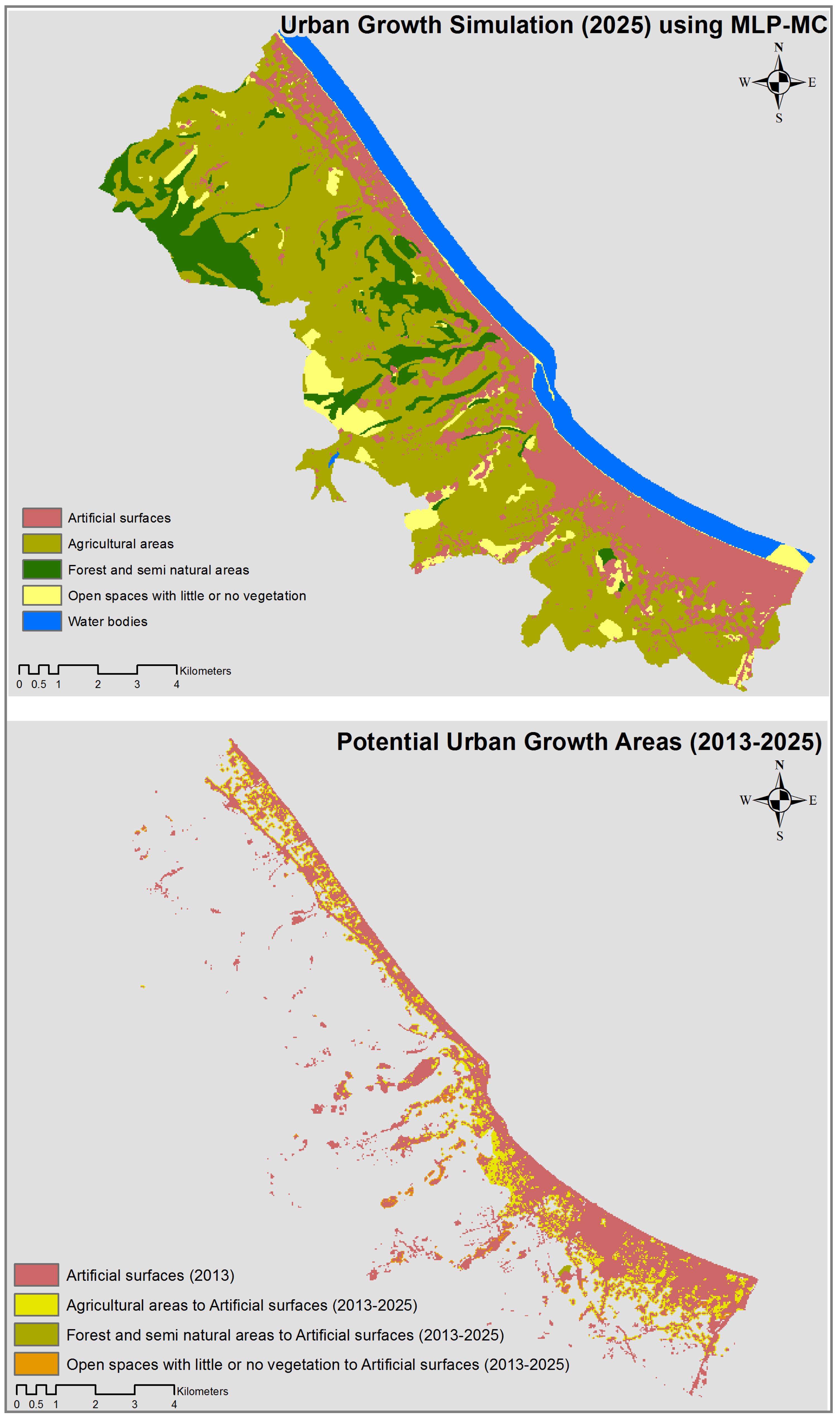
The assessment of the MLP-MC performance for 2013 shows that the simulations for 2025 are sufficiently accurate. The simulation results for 2025 provide significant predictions for the future of Atakum. The 2025 simulation was superimposed on the 2013 LU/LC layer, and urban growth areas predicted for 2013–2025 were extracted, thereby determining which areas will be transformed for urban use (Figure 10). The result of this operation predicted that approximately 511.7 ha of agricultural areas, 4.4 ha of forests and semi-natural areas and 76.3 ha of open spaces with little or no vegetation will be converted for urban use. Based on the changes that occurred in 1989–2000 and 2000–2013 and on the changes predicted from the 2025 simulation results, the transformation to urban use mostly involves agricultural land. A large portion of the land in Atakum is extremely favorable for agriculture, and intense agricultural activities were present on these lands until the 1980s. Since the 1980s, agricultural land has been continuously lost. In fact, the transformation of agricultural land to urban use is a significant problem associated with urbanization in developing countries. 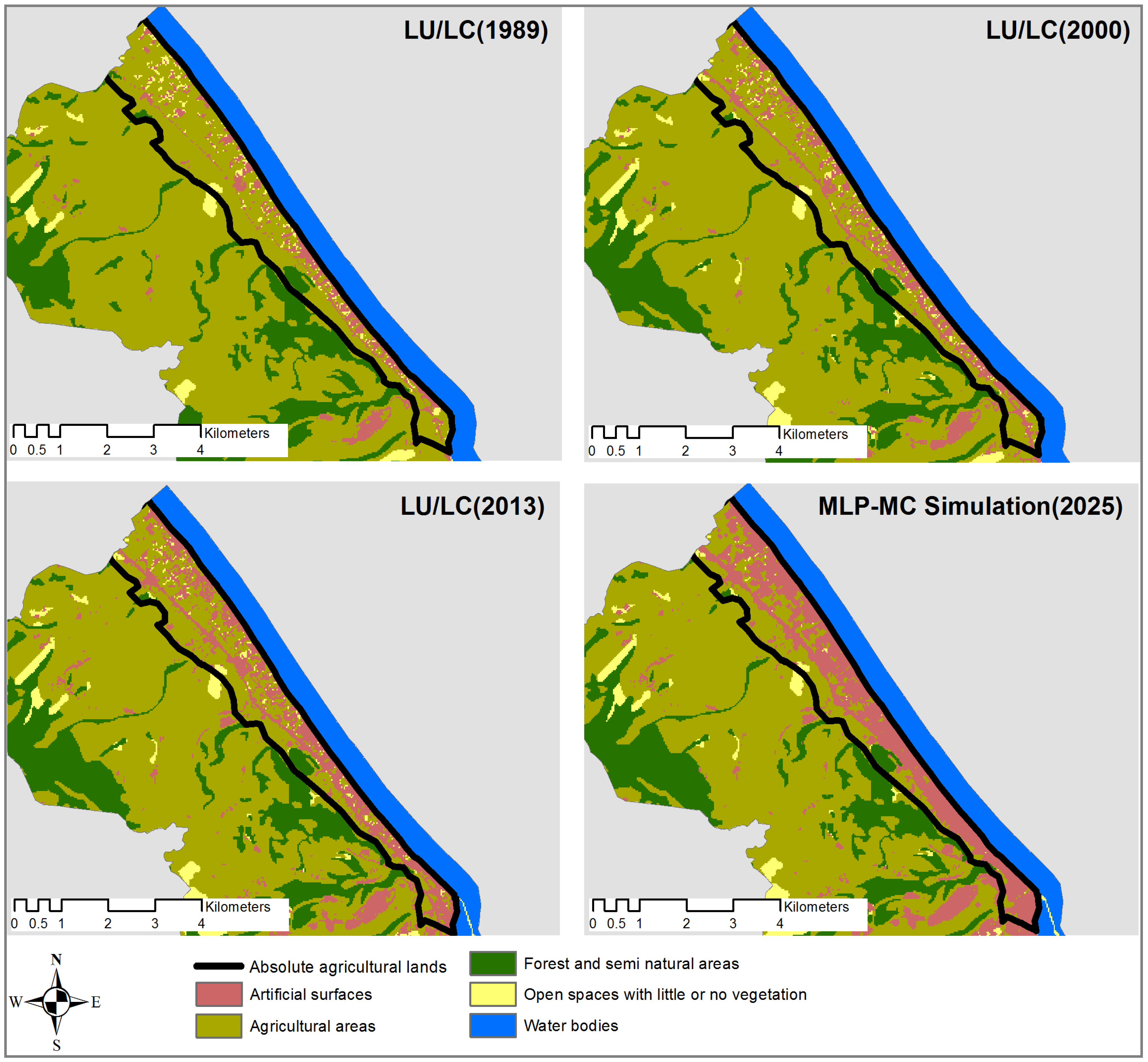Because the areas favorable for agriculture are also suitable for urban growth, the demands for agriculture and settlement are competitive [88]. The natural population increase, the density of the population due to immigrants and the demands for secondary houses/summer houses in the district has produced rapid city growth. However, because of the fertility of the land, all of the areas except forests are used for agriculture. Thus, insufficient free land is available to meet the urban growth demands. Even if the conversion of agricultural land to urban use seems obligatory, this growth is clearly far from environmentally conscious and is devoid of a search for an optimal solution. Although agricultural activities are active on much of the land, the area along the coast west of Ondokuz Mayis University is very fertile and is used as absolute agricultural lands. Although these absolute agricultural lands are expected to be preserved, they are rapidly being zoned for construction. The high slopes to the south of the district have a negative effect on urbanization, and the coastal plains are very attractive for settlement. Thus, many structures were illegally built in these areas until the 1990s, and a mixed pattern of lodging-agriculture formed. Agricultural lands, which became mixed with urban areas over time, were released for construction due to political pressure, administrative mistakes and the lack of awareness at both the public and management levels with regard to the importance and protection of natural resources. The use of these areas for non-agricultural purposes has merely been legalized and tolerated. The LU/LC layers for 1989, 2000, and 2013 and the 2025 simulation layer were overlaid with the absolute agricultural area boundary. The results show that, of the total 999.6 ha of absolute agricultural land, 170.5 ha in 1989, 272.3 ha in 2000, and 397.8 ha in 2013 were classified as urban. These values are predicted to reach 571 ha in 2025. According to this, 173.2 ha absolute agricultural land is at risk. Figure 11 shows the urbanization activities that have occurred since 1989 in absolute agricultural land areas in the region.

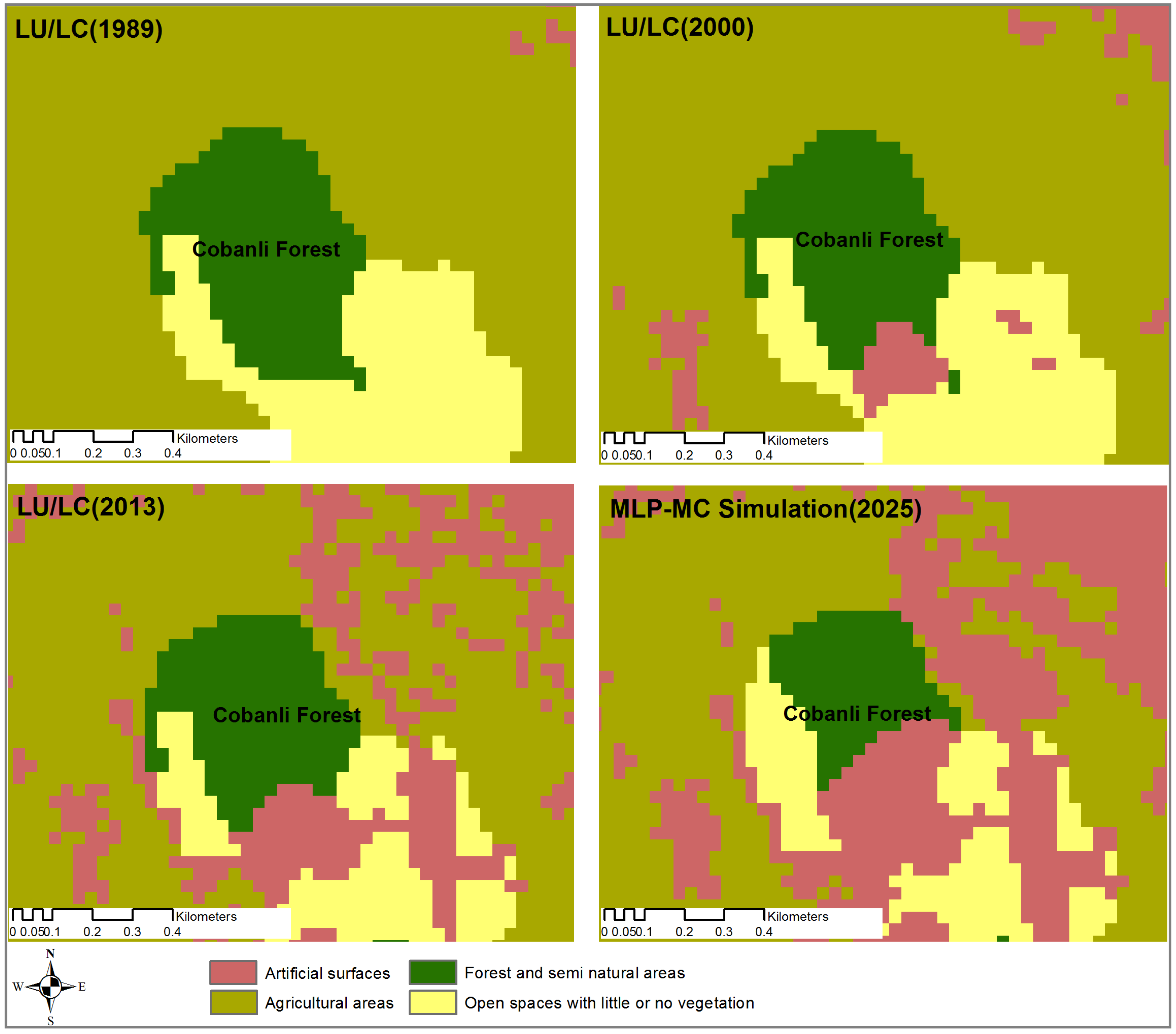
Figure 12. The changes in Cobanli Forest by year as a result of urbanization. The figure shows the gradual forest destruction caused by urbanization.

Figure 12. The changes in Cobanli Forest by year as a result of urbanization. The figure shows the gradual forest destruction caused by urbanization.

Similarly, forests are gradually being destroyed as a result of urbanization. A remarkable example of this process is shown in Figure 12. Cobanli Forest, which was 23.4 ha in 1989, had decreased to 20.6 ha in 2000 and to 18.6 ha in 2013. Additionally, the 2025 simulation results predict that this value will decrease to 11.7 ha. The forest’s proximity to the current urban area and its transportation access allowed the area to be destroyed. The urbanization process in Atakum is rapidly consuming natural resources and damaging the environment. Although the total surface area of forests in Atakum appears to be stable, afforestation is occurring in particular locations, while deforestation is occurring in other areas. Although afforestation appears to compensate for deforestation, the consumption of resources will create irreversible damage. When urbanization is addressed as a whole and when all of the findings are assessed, it can be concluded that all agricultural land will be transformed to urban use in the future, and the mixed pattern of city-agriculture may completely change. If the areas available for urbanization are restricted, then significant increases in the prices of land and buildings may occur [32]. Thus, the urbanization process is a part of the cycle that consumes natural resources, and it should be reviewed by the city planners and managers. Various centers of attraction should be formed to allow for the expansion of the city in areas that are less favorable for agriculture. In other words, expansion should be encouraged to the south to ensure the protection of the current absolute agricultural land and forestland.

6. Conclusions

Around the world, particularly in developing countries, urban growth is associated with particular problems that result in uncontrolled changes. For this reason, determining the current spatial use and urban growth dynamics of cities is among the most important analysis issue in modern urban research. Atakum has experienced rapid urbanization in recent years. As a result of this rapid urbanization, Atakum is faced with the problem of the destruction of natural resources. This study focused on the accurate determination of the future urban growth potential of Atakum and the natural areas that are at risk due to urbanization. Thus, in this study, GIS, remote sensing data and simulation models were combined to understand the dynamics of changes in the urban patterns of Atakum and the urban growth trends that may be encountered through 2025. For this purpose, the urban pattern was examined by using Landsat TM/ETM+/OLI satellite images from 1989, 2000 and 2013 and urban growth simulations were realized using CA-MC and MLP-MC models. The accuracies of the simulation models were assessed for 2013 in the study area, and the 2025 scenario was simulated with the MLP-MC model, which provided superior results. This simulation provides insight into the amount and location of possible changes and spatially and quantitatively identified the risks of urban sprawl. According to simulation results, an increase in the area of artificial surfaces from 1681.9 ha to 2274.3 ha and the destruction of 511.7 ha of agricultural land (173.2 ha of which was absolute agricultural land) and 4.4 ha of forest between 2013 and 2025 was estimated. The results of this study will be considered by city planners, managers and all organizations involved in the decision-making process regarding land use and the creation of prospective land use policies for environmental sustainability, protection of natural resources and preparation of city plans.

This study shows that simulation approaches integrated with remote sensing data and a GIS environment can be effectively used to predict future changes in LU/LC and to analyze the direction, rate and spatial distribution of possible changes. In this study, multiple simulation approaches were used to realize the urban simulation more accurately. Comparison of two different methods enabled the realization of simulation using the better performing method. However, the moderate resolution of the Landsat data negatively affected the accuracy of the LU/LC and the simulation results. To obtain improved results regarding spatio-temporal dynamics, the data quality should be increased and new simulation approaches should be developed.