Global-Scale Evaluation of Roughness Effects on C-Band AMSR-E Observations

Abstract

Quantifying roughness effects on ground surface emissivity is an important step in obtaining high-quality soil moisture products from large-scale passive microwave sensors. In this study, we used a semi-empirical method to evaluate roughness effects (parameterized here by the Hr parameter) on a global scale from AMSR-E (Advanced Microwave Scanning Radiometer for EOS) observations. AMSR-E brightness temperatures at 6.9 GHz obtained from January 2009 to September 2011, together with estimations of soil moisture from the SMOS (Soil Moisture and Ocean Salinity) L3 products and of soil temperature from ECMWF’s (European Centre for Medium-range Weather Forecasting) were used as inputs in a retrieval process. In the first step, we retrieved a parameter (referred to as the a* parameter) accounting for the combined effects of roughness and vegetation. Then, global MODIS NDVI data were used to decouple the effects of vegetation from those of surface roughness. Finally, global maps of the Hr parameters were produced and discussed. Initial results showed that some spatial patterns in the Hr values could be associated with the main vegetation types (higher values of Hr were retrieved generally in forested regions, intermediate values were obtained over crops and grasslands, and lower values were obtained over shrubs and desert) and topography. For instance, over the USA, lower values of Hr were retrieved in relatively flat regions while relatively higher values were retrieved in hilly regions.

1. Introduction

Soil moisture (SM), which plays an essential role in energy transfer between the soil and the atmosphere, is a major variable in hydrological processes [1]. At the global scale, soil moisture is a key variable for weather forecasting [2] and climate predictions [3]. At a regional scale, SM is also important for agriculture and water resources.

The passive microwave remote sensing technique, which has a large spatial coverage and high temporal resolution and is sensitive to surface water content, has been shown to be an efficient approach for large scale soil moisture monitoring [4,5,6]. The measured signal results from the microwave emission of a variety of land cover types in the large (25 km × 25 km) observed pixels. The characteristics of the vegetation (such as vegetation structure and vegetation water content) and the soil (such as soil moisture content, surface roughness and texture) have a significant impact on the surface microwave emissivity [7,8,9,10,11]. Hence, the parameterization of these two effects is the key to obtaining high quality estimates of soil moisture.

The Advanced Microwave Scanning Radiometer (AMSR-E) is a dual-polarized radiometer operating at frequencies of 6.9, 10.7, 18.7, 23.8, 36.5, and 89 GHz. Observations in the C-band range (4–8 GHz) have been used extensively to retrieve soil moisture in regions of low vegetation [4,6,12,13]. However, AMSR-E observations at C-band (6.9 GHz) are strongly affected by man-made radio-frequency interference (RFI)—particularly near large urban areas, requiring filtering these perturbations using RFI indices [4]. AMSR-E has become one of the most important passive microwave sensors for soil moisture monitoring at a global scale due to its long temporal coverage. NASA (National Aeronautics and Space Administration) adopted the algorithm developed by Njoku et al. [4] to retrieve the surface soil moisture based on the AMSR-E data. However, the surface roughness effects are assumed to be constant globally in the algorithm [14,15], which is not consistent with the actual surface conditions, especially in agricultural areas (due to agricultural practices) or deserted regions (due to wind effects) and may cause errors in the SM inversion process [16,17]. Increasing surface roughness effects generally lead to an increase in the measured brightness temperature and to a decrease in the sensitivity of the brightness temperatures to soil moisture [18,19]. Shi et al. [20] found that roughness effects are more significant at high incidence angles and high soil moisture content.

Generally, surface roughness effects are evaluated using physical variables which can be estimated from field measurements, such as the correlation length L_c and the root-mean-square (RMS) height σ_s [21,22,23]. However, traditional measurements of the physical roughness characteristics at the AMSR-E scales are highly uncertain and time consuming [24]. Simplified semi-empirical modelling approaches have also been developed to simulate surface roughness effects. Many studies are based on the use of three main effective parameters to model soil roughness effects: Hr (adimensional and frequency dependant, accounting for roughness intensity), Q (adimensional, accounting for polarization mixing effects) and Nr (adimensional, accounting for angular dependency) [25,26]. Montpetit et al. [27], recently showed that the latter modeling approach was very effective in modeling the signatures of rough soils at AMSR-E frequencies. Several studies estimated the values of the model parameters (Hr, Q, and Nr) from microwave observations over bare fields [21,22] and computed relationships to link these parameters to the physical parameters measured in the fields (mainly σ_s and L_c) [23,24]. However, it is difficult to use these relationships derived from field measurements or modeling approaches calibrated over very small and homogeneous surfaces to model the signatures of rough soils as measured by space-borne systems. At the scale of the footprint of the passive microwave sensors, the pixel includes a variety of land uses and soil and vegetation types, so that it is very difficult to estimate s effective values of σ_s and L_c from ground measurement that can be used to compute the model roughness parameters.

In this paper, we focused on the estimation of the soil roughness parameter Hr. Considering the coarse spatial resolution of the AMSR-E observations, over a given pixel, the time changes in the effects of surface roughness are mixed over a variety of land cover types. Therefore, compared to the time variability, we assumed in this study that the spatial variability of the Hr parameter is more critical. Based on AMSR-E 6.9 GHz TB (brightness temperature) observations, SMOS soil moisture products and ECMWF’s soil temperature, we developed a simple approach to globally estimate the spatial variations in the parameter Hr. The method was first applied over a few sites from the SCAN network in the USA to illustrate the proposed method. In the second step, global maps of the Hr parameter were produced.

2. Data

2.1. AMSR-E

The microwave observations used in this study were measured using the AMSR-E sensor onboard the Aqua satellite. The sensor is a passive microwave radiometer system measuring the horizontally and vertically polarized brightness temperatures at 6.9 GHz, 10.7 GHz, 18.7 GHz, 23.8 GHz, 36.5 GHz, and 89.0 GHz. The antenna scanned conically with an incidence angle fixed at 55°, providing near-global coverage in two days or less. The Aqua’s orbit is sun-synchronous, with equator crossings at 13:30 and 01:30 local solar time. These traits enabled Aqua to observe atmospheric, land, and oceanic parameters. The AMSR-E surface soil moisture product used in this study was the gridded level 3 land surface product at 6.9 GHz [28], which included products on surface soil moisture, vegetation water content and brightness temperatures. This product is projected on the global cylindrical 25 km Equal-Area Scalable Earth Grid (EASE-Grid). Due to a problem with the rotation of its antenna, the AMSR-E instrument on board the Aqua satellite stopped producing data on 4 October 2011. The replacement sensor, AMSR2, which will continue the AMSR-E observation time series, was launched on 18 May 2012. In this study, we selected AMSR-E observations made at the lowest frequency of AMSR-E (6.9 GHz), as it is best suited for SM monitoring [11]. Moreover, this frequency is the closest to the frequency of SMOS (1.4 GHz) which was used for the soil moisture estimations.

It was found that ascending orbit data have larger uncertainties due to surface temperature variations [29,30]. Therefore, the descending orbit brightness temperature observations at C-band were used from January 2010 to September 2011 in this study.

2.2. SMOS

The SMOS satellite is a European Space Agency (ESA) led mission and was launched in November 2009. It is the first satellite specifically dedicated to soil moisture retrievals with an L-band passive radiometer at 1.4 GHz. SMOS provides global coverage in less than three days with a 35–50 km spatial resolution [31,32]. The satellite is polar orbiting with equator crossing times of 6:00 am local solar time (LST) (ascending) and 6:00 pm LST (descending) [33].

SM and vegetation optical depth at nadir (τ_nad) values over land are now available in level 3 products. We used retrieved SM data from the SMOS observations as these data have been shown to be accurate [16,31,34]. Moreover, it is expected that the impact of SM on both the SMOS and AMSRE observations is similar, as these observations are acquired from the same passive microwave technique, even though frequencies are different [16,34]. The level 3 SM projection is also EASE-GRID with a spatial resolution of 25 km × 25 km [35].

For the purpose of using observations with reduced temperature differences between the vegetation canopy and topsoil, the SMOS level 3 ascending daily products were used in this paper [16]. They contain the retrieved parameters (SM, τ_nad), complementary parameters (such as the number of used TB records, surface level modeled TB at 42.5° incidence angle, etc.) and flags. A Data Quality Index (DQX) is associated with each retrieved parameter and could be used to assist assessing the uncertainty of the retrieved parameter. In the SMOS level 3 products, SM is not retrieved in mountainous regions where topography effects are strong (a topographic index is used to filter out these data [36,37]). Similarly, SM is not retrieved in regions covered by dense forests, where the sensitivity to SM is very low, or in pixels where the forest fraction exceeds 60% [10].

2.3. MODIS NDVI

The MODIS/Terra Normalized Difference Vegetation Index (NDVI) product (MOD13C1) is used for monitoring vegetation conditions globally [38]. NDVI is calculated as:

$$NDVI=\frac{{\rho }_{NIR}-{\rho }_{Red}}{{\rho }_{NIR}+{\rho }_{Red}}$$

(1)

where ρ_NIR is the reflectance in the near Infra-Red band, taken from band 2 of MODIS (841–876 nm) and ρ_Red the reflectance in the red band, taken from band 1 of MODIS (620–670 nm). ρ_Red is mainly sensitive to the amount of chlorophyll and ρ_NIR depends on the amount of leaf area. Thus, NDVI is a good indicator of green leaf area [39]. The MODIS NDVI product contains atmospherically corrected bi-directional surface reflectance masked for water, clouds, and cloud shadows. Global MOD13C1 data are cloud-free spatial composites of the gridded 16-day product and are provided as a level-3 product projected on a 0.05 degree (5600-m) geographic Climate Modeling Grid (CMG). The quality assurance (QA) data, provided in the NDVI dataset, include cloud and snow cover percentages, aerosol information and other factors.

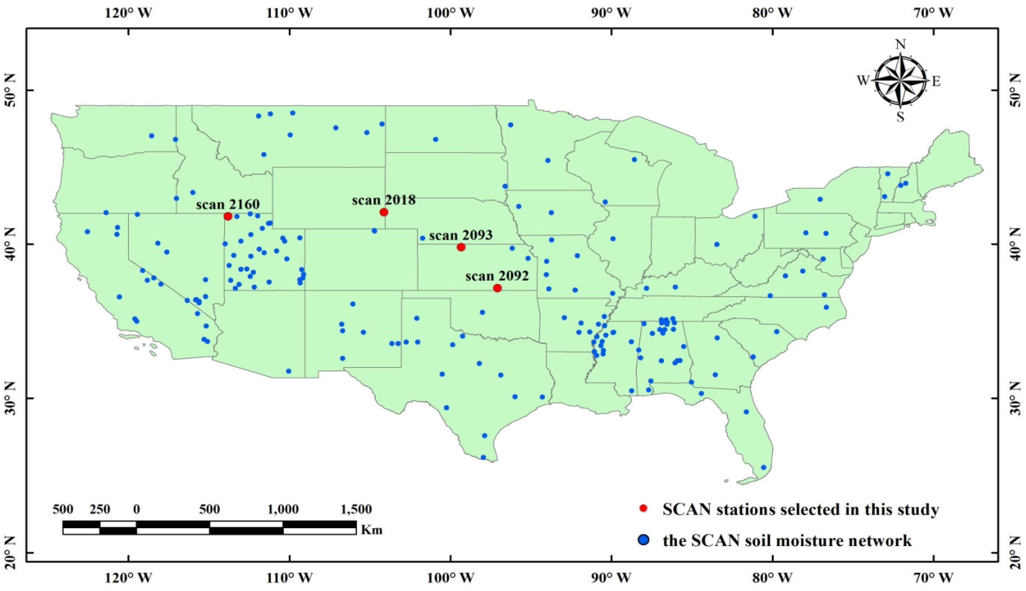
2.4. The SCAN Network

In this study, we selected four stations from the Soil Climate Analysis Network (SCAN, http://www.wcc.nrcs.usda.gov) in the USA [40] to carry out a preliminary evaluation of the method. We selected stations where the nominal (bare soil and low vegetation) fraction is above 90% (Figure 1) and where the vegetation covers (crops or grassland) are relatively homogeneous at the scale of the AMSR-E and SMOS pixels.

Figure 1. General map of the SCAN Soil Moisture network (blue labels) and the four SCAN stations selected in this study (red labels).

Figure 1. General map of the SCAN Soil Moisture network (blue labels) and the four SCAN stations selected in this study (red labels).

The selected four stations for this study are located in Utah (SCAN 2016), Wyoming (SCAN 2018), and Kansas (SCAN 2093 and SCAN 2092).

SCAN site 2092 is located in Cowley in a relatively flat area at an altitude of 364 m (above sea level, a.s.l.). Land use is mainly cropping and the forest cover fraction in this area is about 1%. Soil is dominated by sand (soil texture is 72.4% sand and 7.5% clay).

Table 1. Description of the DGG nodes representative of the selected SCAN sites from [41] (FNO: Nominal fraction, FFO: Forest fraction, FWO: Water fraction).

Node	Station Name	Site	Fractions				Cover Type	Texture		State
			FNO	FFO	FWO	Other		Sand (%)	Clay (%)
172276	Grouse Creek	SCAN 2160	100	0	0	0	Grassland (mountain)	--	--	Utah
186675	Torrington	SCAN 2018	100	0	0	0	Grassland	80.3	5.5	Wyoming
203609	Phillipsburg	SCAN 2093	98	0	0	2	Crops	5.8	22.4	Kansas
218480	Abrams	SCAN 2092	97	1	0	2	Crops	72.4	7.5	Kansas

Table 1. Description of the DGG nodes representative of the selected SCAN sites from [41] (FNO: Nominal fraction, FFO: Forest fraction, FWO: Water fraction).

Node	Station Name	Site	Fractions				Cover Type	Texture		State
			FNO	FFO	FWO	Other		Sand (%)	Clay (%)
172276	Grouse Creek	SCAN 2160	100	0	0	0	Grassland (mountain)	--	--	Utah
186675	Torrington	SCAN 2018	100	0	0	0	Grassland	80.3	5.5	Wyoming
203609	Phillipsburg	SCAN 2093	98	0	0	2	Crops	5.8	22.4	Kansas
218480	Abrams	SCAN 2092	97	1	0	2	Crops	72.4	7.5	Kansas

The SCAN 2093 site, located in Phillips, is mainly covered by crops. The altitude of this site is 605 m (a.s.l.). SCAN 2018 site is located in Wyoming at an altitude of 1300 m (a.s.l.) and the surface fraction is 100% nominal (i.e., bare soil and low vegetation surfaces). The land cover is mainly grassland with 80.3% sand and 5.5% clay. The last SCAN 2016 site is located in Utah at an altitude of 1781 m (a.s.l.) in a mountainous region. The surface is totally covered by grassland. The details concerning the soil and vegetation characteristics are summarized in Table 1 for the four selected sites.

2.5. Ancillary Products

This study used a custom made climate data product (AUX_ECMWF) from the European Centre for Medium-range Weather Forecasting (ECMWF) as SMOS ancillary data. The ECMWF provides medium range global forecasts of environmental variables such as SM, evaporation, skin temperature, root zone soil temperature, precipitation, etc. The top 7 cm layer soil temperature selected in this study was obtained via the SMOS L3 pre-processor that computes spatio-temporal averaging of the ECMWF forecast products on the EASE grid used for the SMOS Level 3 products [42].

The global land cover map was obtained from the Second Global Soil Wetness Program (GSWP2). The data set is based on the International Geosphere-Biosphere Programm (IGBP) classification system and contains 12 land cover types. The spatial resolution is 1 degree [43].

The global soil clay map was estimated from the Food Agriculture Organization (FAO) [44], and we used a global digital elevation model (DEM) resulting from Global 30 Arc-Second Elevation (GTOPO30) computed at the U.S. Geological Survey’s EROS Data Center (USGS) (available at https://lta.cr.usgs.gov/GTOPO30). The elevations we used in GTOPO30 were spaced at 30-arc seconds (approximately 1 kilometer) [45].

2.6. Remote Sensing Data Pre-Processing

RFI originating from man-made emissions in the protected/shared bands (e.g., satellite transmissions, aircraft communications, radar, TV radio-links, FM broadcast, and wireless camera monitoring systems) perturbs the natural microwave emission emitted by the Earth’s surface and measured by passive microwave systems [16,46,47]. Some studies have shown that RFI has a significant impact on the brightness temperatures at the C-band and L-band [46,48,49]. RFI contamination at the C-band were found to be highly prevalent in the U.S., Southwest Asia, and the Middle East, with occurrences in Europe seemingly associated with some urban locations [46,48,49]. In this study, C-band AMSR-E observations affected by strong and moderate RFI effects were removed by calculating the RFI Index derived from the difference between the brightness temperatures at 6.9 and 10.7 GHz [46,48]. Quality control was applied to the SMOS L3 SM products. The RFI flag provided in the SMOS L3 data set was used to filter out the RFI effects. Moreover, the Level 3 DQX flag was used to evaluate the uncertainty associated with the SM retrievals; SMOSL3 data were rejected if one of the following conditions was fulfilled: (i) DQX > 0.06, (ii) DQX is equal to fill value, and (iii) probability of RFI (RFI_Prob) > 30% [16].

As the performances of C-band sensors to sense SM through dense forests is low, the AMSR-E pixels in densely forested regions were masked based on the GSWP-2 global land cover maps [43]. In this study, the regions classified as broadleaf evergreen forest were masked.

In order to have enough NDVI data to match with the data from the other datasets, we linearly interpolated the 16-day NDVI products into a 4-day product in this study. In the NDVI time series over each pixel, all values lower than 0 (influenced by ice, snow and frost effects) were removed. All the datasets were re-projected to the cylindrical EASE-Grid projections using a nearest neighbor approach [50].

3. Method

This study was based on the τ − ω [22] model with the assumption of a low influence from atmospheric effects and neglecting the multiple scattering effects in the vegetation. The brightness temperature TB_p can be expressed as a three-component model (Equation (2)). The first part is the upward radiation from vegetation, the second part is the downward vegetation emission reflected by the soil and then attenuated by the canopy, and the last part is the soil emission attenuated by the vegetation canopy.

$$T{B}_{\left(p,\theta \right)}=\left(1-{\omega }_p\right)\left(1-{\gamma }_{\left(p,\theta \right)}\right)T_C{\gamma }_{\left(p,\theta \right)}{r}_{G\left(p,\theta \right)}+\left(1-{\omega }_p\right)\left(1-{\gamma }_{\left(p,\theta \right)}\right)T_C+\left(1-r_{G\left(P,\theta \right)}\right){\gamma }_{\left(P,\theta \right)}{T}_G$$

(2)

where T_G and T_C are the effective soil and vegetation temperature, r_G is the soil reflectivity, γ is the vegetation attenuation factor and ω is the single scattering albedo of the canopy; θ is the incidence angle of the observations. The parameter ω accounts for the effects of canopy volume scattering [22]. However, there is limited information on the temporal or canopy type variability of this parameter, and most of the SM retrieval algorithms considered the use of a constant global value [51]. Van de Griend and Owe [52] showed that ω had a low effects on the range of the emitted radiation from vegetated surfaces at microwave wavelengths [7,51]. For simplicity, as in several other studies at C-band, it is assumed in this study that ω, considered here as an effective parameter [53], is equal to zero [1,7,52]. Furthermore, T_C and T_G are assumed to be equal at 6 am and represented as T [54]. These assumptions lead to the following simplified equation [55]:

$$T{B}_{\left(P,\theta \right)}=\left(1-{\gamma }_{\left(p,\theta \right)}^2{r}_{G\left(p,\theta \right)}\right)T$$

(3)

The soil reflectivity r_G can be written as a function of the reflectivity of a flat surface $r_{G(p,\theta )}^{*}$, a set of four soil roughness parameters (Hr, Q, Nrp, p = V or p = H), incidence angle θ and polarization p, as [19]:

$$r_{G\left(P,\theta \right)}=\left[\left(1-Q\right)r_{G\left(p,\theta \right)}^{*}+Q{r}_{G\left(q,\theta \right)}^{*}\right]\times exp\left(-Hr co{s}^{N{r}_p}\left(\theta \right)\right)$$

(4)

where Q is the polarization mixing parameter [7], Hr is a parameter related to the intensity of the roughness effects and Nr_p expresses the angular dependency of the roughness effects [56]. An increase in the value of the Q parameter generally leads to a decrease in the difference between TB_H and TB_V (TB_H increases and TB_V decreases). Wang et al. [57] have found that the frequency dependence of Q is strong and relatively small values for Q were obtained, ranging from 0 to 0.12 at L-band and from 0 to 0.3 at C-band. More recently, Montpetit et al. [27] have found that the value Q = 0.075 can be used over a large frequency range (1.4–90 GHz). In this study, we considered the value of Q is equal to zero, but a sensitivity analysis is made for Q varying from 0 to 0.3. Following the result obtained by [23], the values of Nrp for the H and V polarizations were set equal, and we assumed that Nr_H = Nr_V = 0 [23]. According to the Fresnel equations, $r_{G(p,\theta )}^{*}$ at a specific incidence angle is only related to the soil dielectric properties (ε_p). In the present study, ε_p was estimated using the Mironov model [57]. The inputs of the Mironov model in this study were (i) SM estimated from the SMOS observations, (ii) the soil effective temperature provided by the ECMWF products and (iii) the clay fraction (%) estimated from the FAO maps.

The vegetation attenuation factor (γ) was expressed as the function of the optical depth τ_p as:

$${\gamma }_{\left(p,\theta \right)}=exp\left(-{\tau }_p/cos\left(\theta \right)\right)$$

(5)

and the vegetation optical depth τ_p can be calculated from the optical depth at nadir (at θ = 0) as [26]:

$${\tau }_p={\tau }_{nad}\left(co{s}^2\left(\theta \right)+t{t}_{p}si{n}^2\left(\theta \right)\right)$$

(6)

where tt_p is a specific vegetation parameter accounting for the effects of the vegetation structure. The tt_p parameters allow accounting for the dependence of τ_nad on incidence angle. A value of tt_p > 1 or tt_p < 1 will correspond, respectively, to an increasing or decreasing trend of τ_nad as a function of θ, and the case tt_H = tt_V = 1 corresponds to isotropic conditions, when the optical depth of the standing canopy is assumed to be independent of both polarizations and incidence angles. Some experimental evidence has shown that there is a difference in vegetation attenuation properties between the H and V polarizations over agricultural fields, mainly for vertical stem-dominated vegetation (such as wheat or corn) [14]. However, the canopy and stem structure for most crops and naturally occurring vegetation are randomly oriented. Moreover, considering that at coarse spatial resolution the pixel includes a variety of vegetation types, so that the specific effects related to the structure of a variety of vegetation canopies are mixed together, it is reasonable to assume that the optical depth is polarization-independent (tt_H = tt_V = 1) [51,52,58].

Previous studies, such as Schmugge et al. [59] and Jackson et al. [6] combined the vegetation optical depth and roughness effects within a single parameter (referred to as the α parameter) to retrieve soil moisture. Similarly, Njoku & Chan [7] and Saleh et al. [60] used this α parameter to approximate the combined effects of vegetation and roughness. Consequently, in this study, substituting Equations (5) and (6) in Equation (3), we can obtain:

$$T{B}_{\left(P,\theta \right)}=T\left[1-r_{G\left(p,\theta \right)}^{\prime }a\right]$$

(7)

with

$$\text{a}\left(\text{θ}\right)=\text{exp}\left(-\frac{2{\text{τ}}_{\text{nad}}}{\text{cos}\left(\text{θ}\right)}-\text{Hr}\right)$$

(8)

Considering the H and V polarizations, the a parameter can be derived as [61]:

$$\text{a}\left(\text{θ}\right)=\frac{{\text{TB}}_{\left(\text{V},\text{θ}\right)}-{\text{TB}}_{\left(\text{H},\text{θ}\right)}}{{\text{TB}}_{\left(\text{V},\text{θ}\right)}{\text{r}}_{\text{G}\left(\text{H},\text{θ}\right)}^{\prime }-{\text{TB}}_{\left(\text{H},\text{θ}\right)}{\text{r}}_{\text{G}\left(\text{V},\text{θ}\right)}^{\prime }}$$

(9)

In the following of this study we considered the parameter a* defined as follows:

$$a^{*}\left(\theta \right)=-log\left(a\left(\theta \right)\right)=\frac{2{\tau }_{nad}}{cos\left(\theta \right)}+Hr$$

(10)

From this equation, a*(θ) can be seen as a parameter accounting for the combined effects of vegetation (through the τ_nad parameter) and surface roughness (through the Hr parameter) [26]. The parameter a*(θ) at a given incidence angle can be directly calculated from the horizontal and vertical polarization brightness temperatures using Equation (9). In this study, the a*(θ) parameter was calculated with only one angle and for ease of reading it is noted a* in the following of the text.

We used the NDVI index in an attempt to decouple the vegetation and surface roughness effects in Equation (10). To this aim, we assumed that optical depth can be linearly related to the vegetation index NDVI [39,62,63]. Note that errors may arise from this assumption, as a linear relationship between optical depth and NDVI is only suitable for vegetation canopies with a rather low biomass [63]. In particular, NDVI is likely to saturate more rapidly than optical depth (due primarily to the deeper penetration capabilities of the microwave radiations) over dense canopies in forested regions. We assumed too that the attenuation effects of vegetation are very low for low values of NDVI, so that roughness effects are dominant (a* ≈ Hr) when VI ≈ 0.

Using these assumptions, at a given incidence angle, the parameter a* can be expressed as a function of NDVI over each pixel as:

$$a^{*}=A\times NDVI+Hr$$

(11)

where A is a slope parameter which has to be calibrated over each pixel.

Equation (11) was used to compute the value of Hr over each pixel. For this purpose, a standard statistical procedure was applied to compute the slope and intercept of regression Equation (11) using values of the NDVI index estimated from MODIS and values of a* computed from the AMSR-E observations (using Equation (9)).

In this process, we considered two main cases:

• “Bare or sparsely vegetated surfaces”, corresponding here to the case when the effects of the vegetation layer, could be considered negligible over a sufficient period of time (this case was arbitrarily defined here as when 15% of the NDVI values were lower than 0.07 in the whole NDVI time series [64]).

In that case, we set the surface roughness Hr as the average value of a* under the condition of NDVI values lower than 0.07. This case included the case of deserts, where the NDVI values where always lower than 0.07. In that latter case, we set the value of Hr as the average value of a*.

2.

“Vegetated surfaces” corresponding here to the case when the effects of the vegetation layer are significant over most of the dates of the considered dataset (case defined as: more than 85% of the NDVI values exceed the threshold value of 0.07).

In that case, we set the surface roughness Hr as the intercept of the regression Equation (11), linking a* to NDVI. Note that the values of Hr were computed only over nodes where (i) the correlation was significant (p-value < 0.05) and where (ii) the coefficient of determination R² was higher than a threshold value set arbitrarily here to 0.2 (R² > 0.2). This filtering was conducted in order to compute values of Hr from the value of the intercept of the regression line only when there was a well-defined correlation between a* and NDVI.

Following that procedure over all pixels, we could compute a global map of the parameter Hr, except over regions of dense forests, which were masked out.

4. Results and Discussion

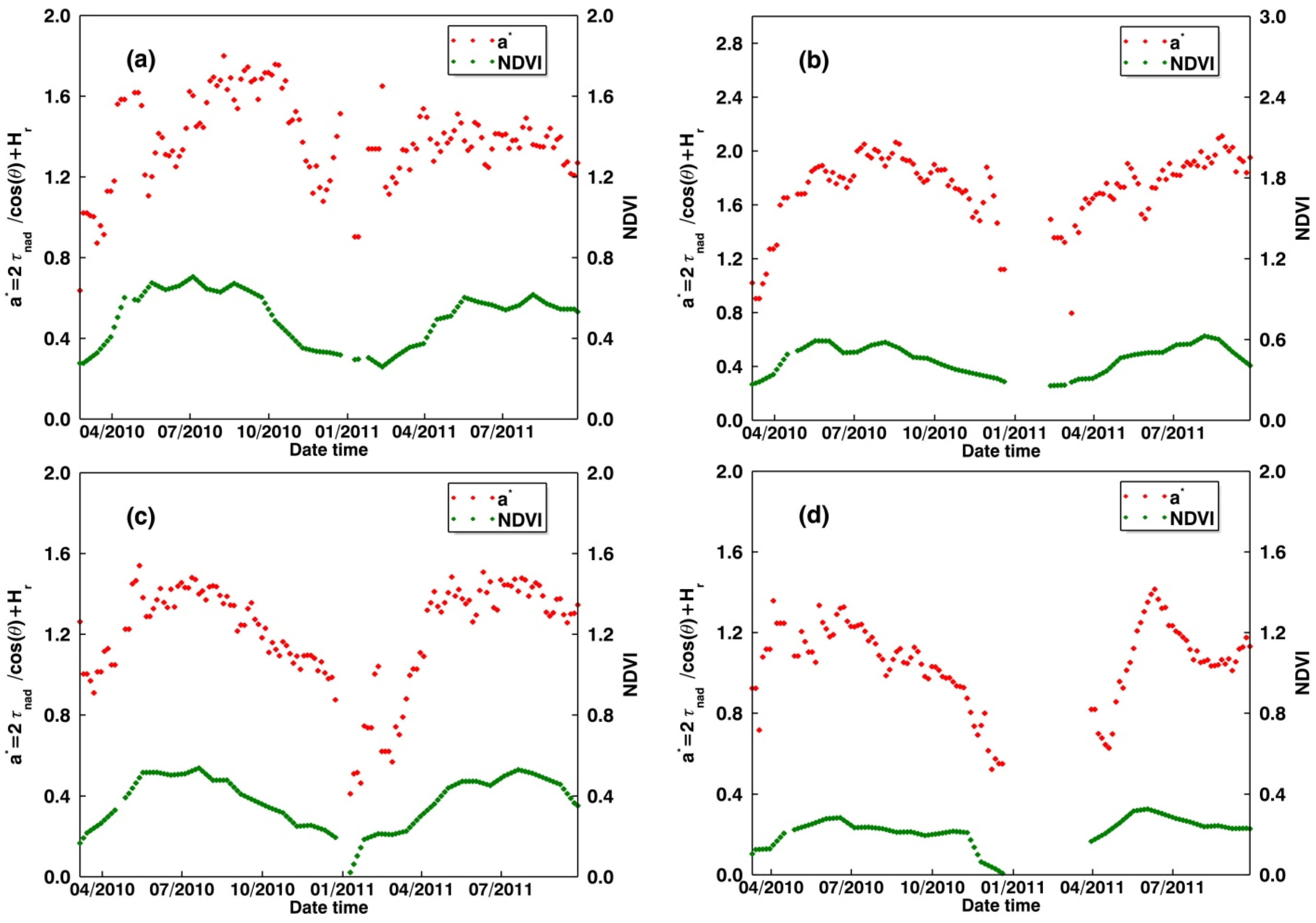
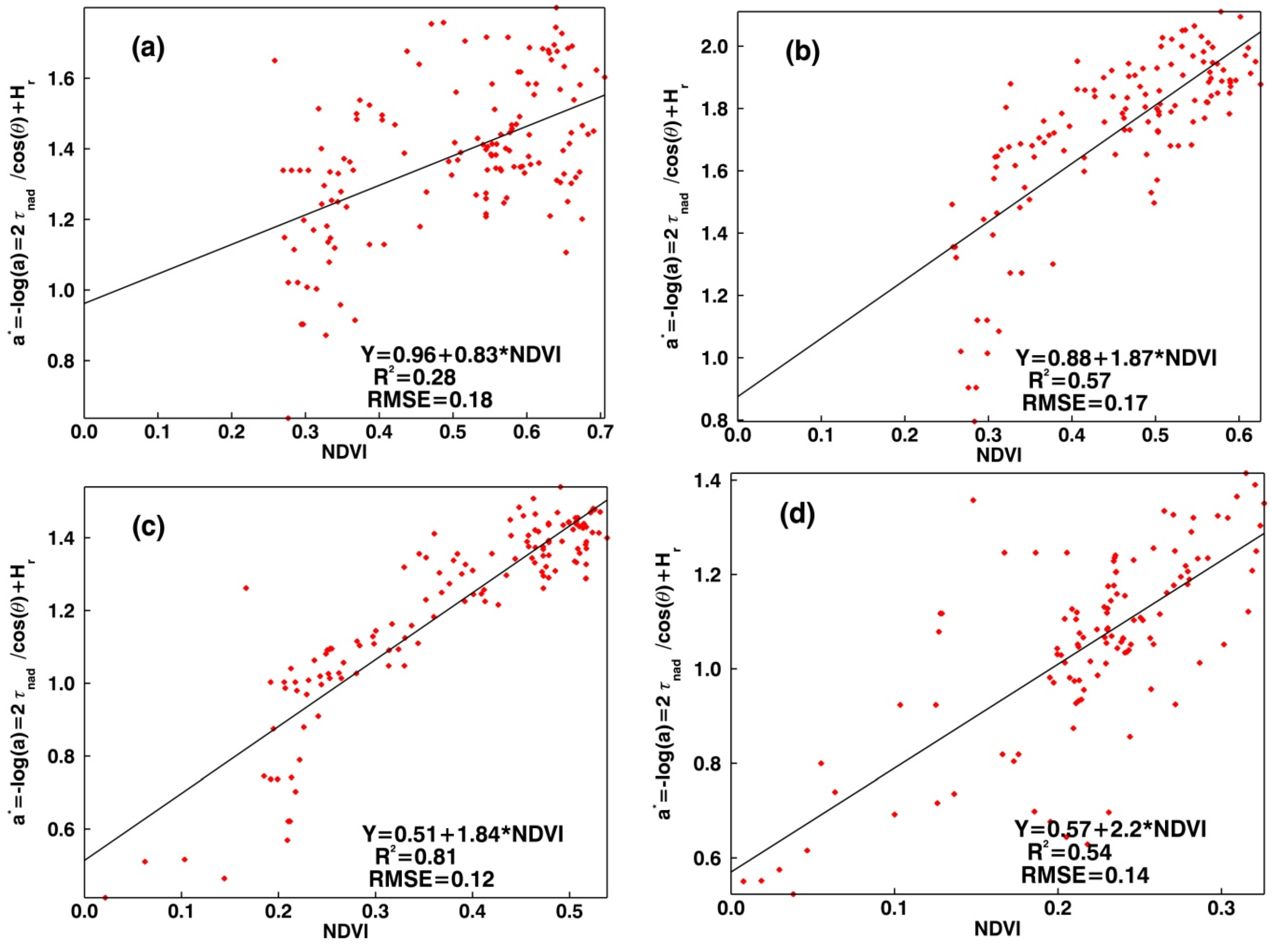
4.1. Results Obtained Over the Selected SCAN Sites

To illustrate the use of the method developed in this study, Figure 2a–d show a comparison between the retrieved values of a*, using the equations described above, and the MODIS NDVI values over the four selected SCAN sites, from January 2010 to September 2011. Gaps in the time series of and NDVI values in Figure 2 were due to filtering, particularly for the effects of snow and frozen soil. It can be seen that the retrieved values of a* showed an overall increase from April to August, then started to decrease and reached a minimum around the end of January, for both years (2010 and 2011). This temporal change pattern was similar with that of NDVI (Figure 2), indicating that the general trend of a* is mainly determined by the growth and senescence of vegetation. The values of a* and NDVI appeared to start increasing at the same time, but a* reached a peak slightly later than NDVI. The difference in peak time may be explained by the fact that microwave observations are sensitive the changes in the vegetation water content of the whole plant (including stem and fruit growth) while the NDVI index is mainly related to the development of green leaves [26,36,39]. These effects have been observed from experimental in-situ data over soybean and wheat [26,65] and from the SMOS observations [39].

Figure 2. Time series of the a* parameter and of the MODIS NDVI over SCAN sites, (a) 2092, (b) 2093, (c) 2018, and (d) 2160 (January 2010–September 2011).

Figure 2. Time series of the a* parameter and of the MODIS NDVI over SCAN sites, (a) 2092, (b) 2093, (c) 2018, and (d) 2160 (January 2010–September 2011).

The scatter plots and the linear regressions between a* and NDVI are showed in Figure 3a–d for the four SCAN sites. It can be seen that there is a good general linear relationship between the values of a* and NDVI over the different sites (R² ranging from 0.28 to 0.81), even though there is a slight time lag in the general trend of the two variables (as noted above). It can be seen that there are few data close to zero, i.e., for low NDVI values. It is likely this can be explained by the fact the effects of vegetation remained significant over the whole year, especially for sites including permanent grasslands (SCAN sites 2160 and 2018). This can be also explained by the fact that time periods with low vegetation development correspond to time periods with snow and frozen soil conditions, which were filtered out in the data sets.

Figure 3. Scatter plot illustrating the relationship between the a* parameter and MODIS NDVI over SCAN sites (a) 2092, (b) 2093, (c) 2018, and (d) 2160 (January 2010–September 2011).

Figure 3. Scatter plot illustrating the relationship between the a* parameter and MODIS NDVI over SCAN sites (a) 2092, (b) 2093, (c) 2018, and (d) 2160 (January 2010–September 2011).

As very few values of NDVI were lower than the threshold of 0.07, the value of Hr over the different sites was computed as the intercept of the regression line between a* and NDVI. The values of Hr are in the range between ~ 0.5 for sites covered mainly by grassland (Hr = 0.51 for SCAN site 2018 and Hr = 0.57 for SCAN site 2016) and ~0.9 for sites covered mainly by cropland (Hr = 0.96 for SCAN site 2092 and Hr = 0.86 for SCAN site 2093).

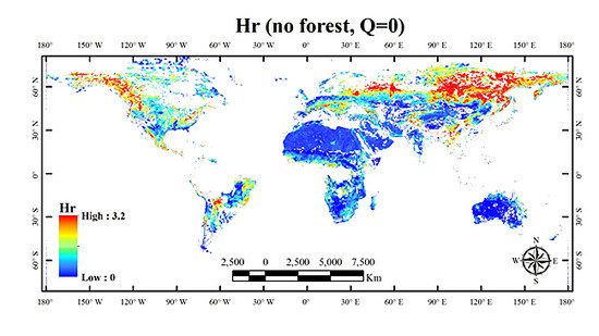
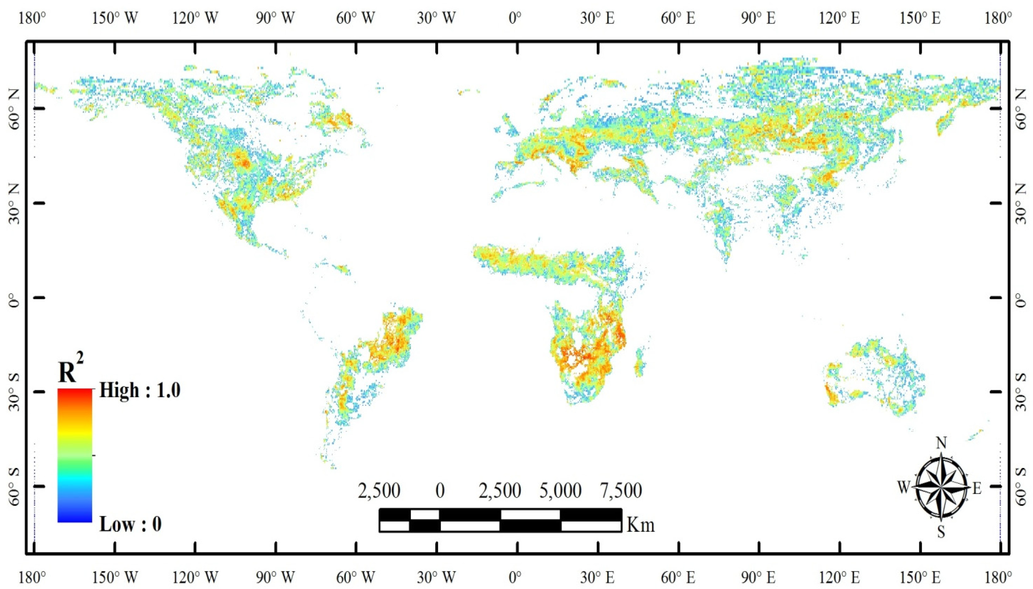
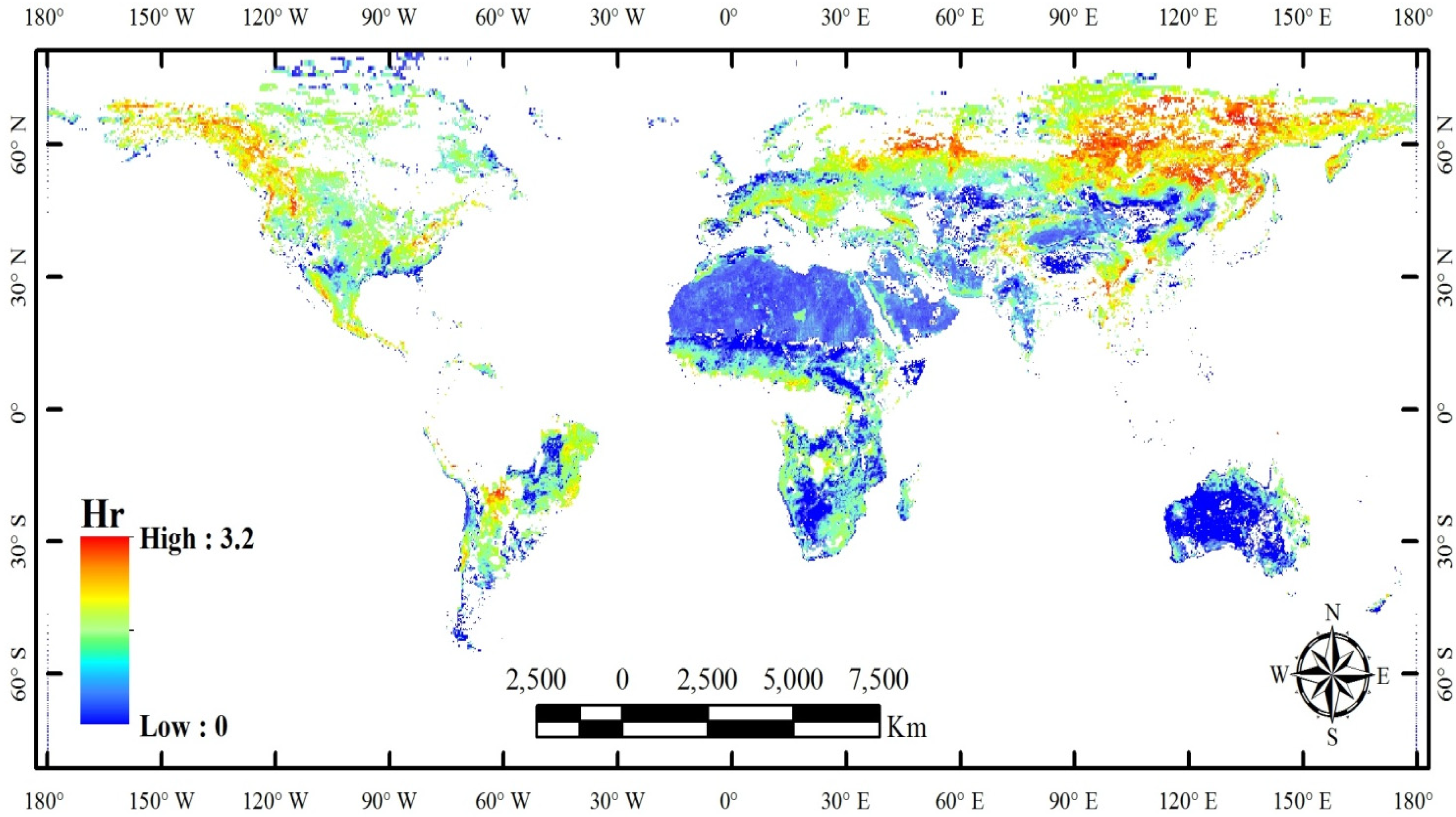
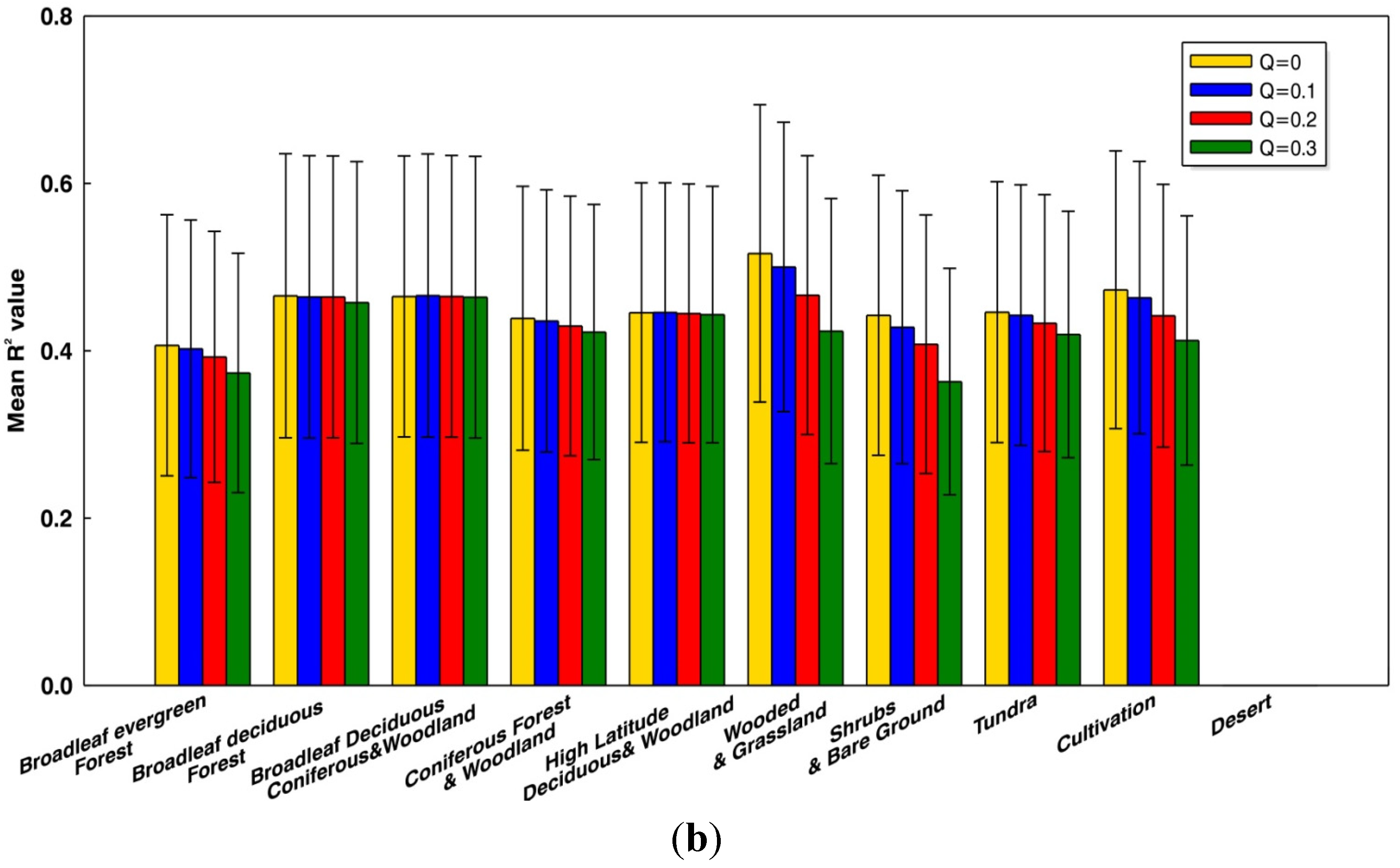
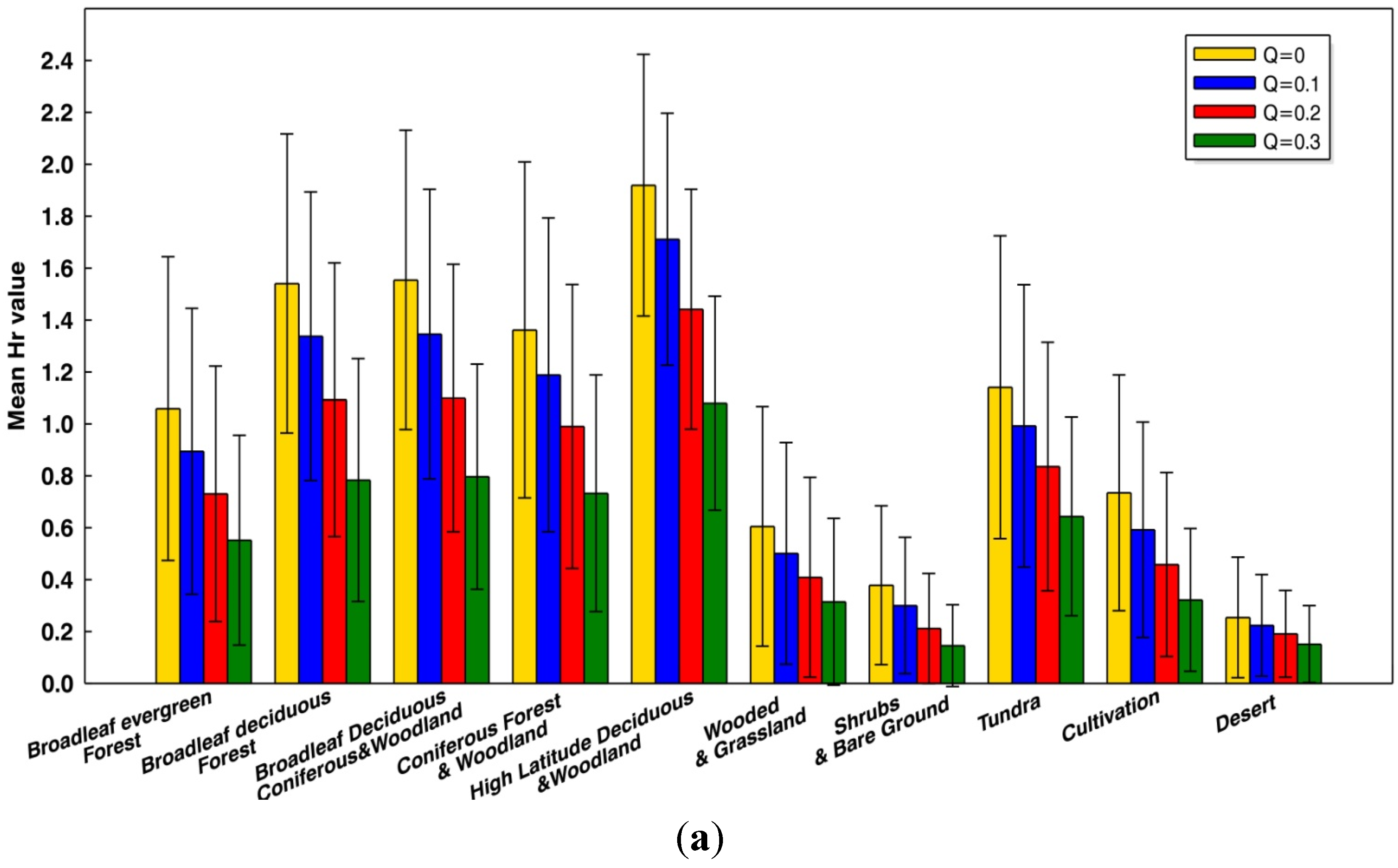
4.2. Global Map of the Hr Values

Using the same approach as the one illustrated above for the four selected sites of the SCAN network, the value of Hr was estimated at a global scale.

As described in section 3, two cases were considered to produce the value of Hr: (1) “Bare or sparsely vegetated surfaces” and (2) “Vegetated surfaces”. In case (1), Hr was computed as an average of a* for dates with low vegetation effects (parameterized here arbitrarily as NDVi < 0.07). In case (2), the vegetation effects are always significant so that a* includes both the effects of roughness and vegetation. In that latter case, Hr was computed as the intercept of regression Equation (11) relating a* and NDVI.

It was found that at a global scale, 24% of the pixels (i.e., 25710 over 107135 pixels) correspond to case (1), while 76% (i.e., 81425 over 107135 pixels) correspond to case (2).

The results of the analysis are summarized in Table 2 as a function of the different types of vegetation for the case Q = 0. We obtained an average value of R² varying between 0.41 and 0.52 for the regression equation relating a* to NDVI for the different land cover types (except for deserts where this relationship could not be computed), and the average value of Hr varied from 0.26 (over desert region) to 1.92 (over high latitude deciduous forest and woodland). It can be seen that Hr was generally higher over forest biomes (Hr ~ 1.35–1.92), such as broadleaf evergreen forests, broadleaf deciduous forests, mixed coniferous, coniferous forests, high latitude deciduous forests and lower over the land covers as wooded and grasslands (Hr = 0.61) and cultivation (Hr = 0.74). The lowest values of Hr were obtained over shrubs & bare ground (Hr ~ 0.38) and deserts (Hr ~ 0.26). Note the mean values of Hr had almost no differences between grassland and cropland (only a 0.1 difference).

Table 2. Mean values of Hr and of the R² for the linear regression between a* and NDVI for a variety of biomes as defined in [43]. Hr and R² values were averaged over all pixels corresponding to the different biomes (N = number of pixels considered in the computation).

Classification	Q = 0
	Mean Hr	Mean R2	N
broadleaf evergreen forest	1.06	0.41	2098
broadleaf deciduous forest & woodland	1.54	0.47	2526
mixed coniferous & broadleaf deciduous forest & woodland	1.55	0.47	2403
coniferous forest & woodland	1.36	0.44	4688
high latitude Deciduous forest & woodland	1.92	0.44	3674
wooded & grassland	0.61	0.52	30,384
shrubs & bare ground	0.38	0.44	4827
Tundra	1.14	0.45	8362
Cultivation	0.74	0.47	22,099
Desert	0.26	--	25,128

Table 2. Mean values of Hr and of the R² for the linear regression between a* and NDVI for a variety of biomes as defined in [43]. Hr and R² values were averaged over all pixels corresponding to the different biomes (N = number of pixels considered in the computation).

Classification	Q = 0
	Mean Hr	Mean R2	N
broadleaf evergreen forest	1.06	0.41	2098
broadleaf deciduous forest & woodland	1.54	0.47	2526
mixed coniferous & broadleaf deciduous forest & woodland	1.55	0.47	2403
coniferous forest & woodland	1.36	0.44	4688
high latitude Deciduous forest & woodland	1.92	0.44	3674
wooded & grassland	0.61	0.52	30,384
shrubs & bare ground	0.38	0.44	4827
Tundra	1.14	0.45	8362
Cultivation	0.74	0.47	22,099
Desert	0.26	--	25,128

According to the method defined above, global maps of the R² coefficient and of the Hr parameter are shown in, respectively, Figure 4 and Figure 5, for the case Q = 0.

It can be seen (Figure 4) that high correlation values (R²) for regression Equation (11) were generally obtained over the USA, tropical regions in Africa, Eastern and Western Europe, central eastern South America and Mongolian plateau. As mentioned before, it should be noted that the R² coefficient was not computed in desert regions and the densely forested regions were masked out. There were some other factors influencing R², such as the uncertainties in the SMOS SM data and the ECMWF soil temperature that we used as inputs, the poor resolution of the passive microwave sensors (25 km × 25 km), the measured signal resulting from the microwave emission of a variety of land cover types in the observed pixels, and some pixels being affected by the effects of topography or by dense forests. Consistently with the results given in Figure 4, the global map of the Hr values (Figure 5) showed that the lowest values of Hr were obtained in deserted or low vegetated regions (e.g., Australia and Sahara desert). The highest values were obtained in forested areas and in the Northern regions.

Figure 4. Global map of the coefficient of determination (R²) of the relationship between a* and NDVI (AMSR-E observations at C-band, January 2010–September 2011), for the case Q = 0.

Figure 4. Global map of the coefficient of determination (R²) of the relationship between a* and NDVI (AMSR-E observations at C-band, January 2010–September 2011), for the case Q = 0.

Figure 5. Global map of the retrieved roughness parameter Hr at C-band (AMSR-E observations, January 2010–September 2011), for the case Q = 0.

Figure 5. Global map of the retrieved roughness parameter Hr at C-band (AMSR-E observations, January 2010–September 2011), for the case Q = 0.

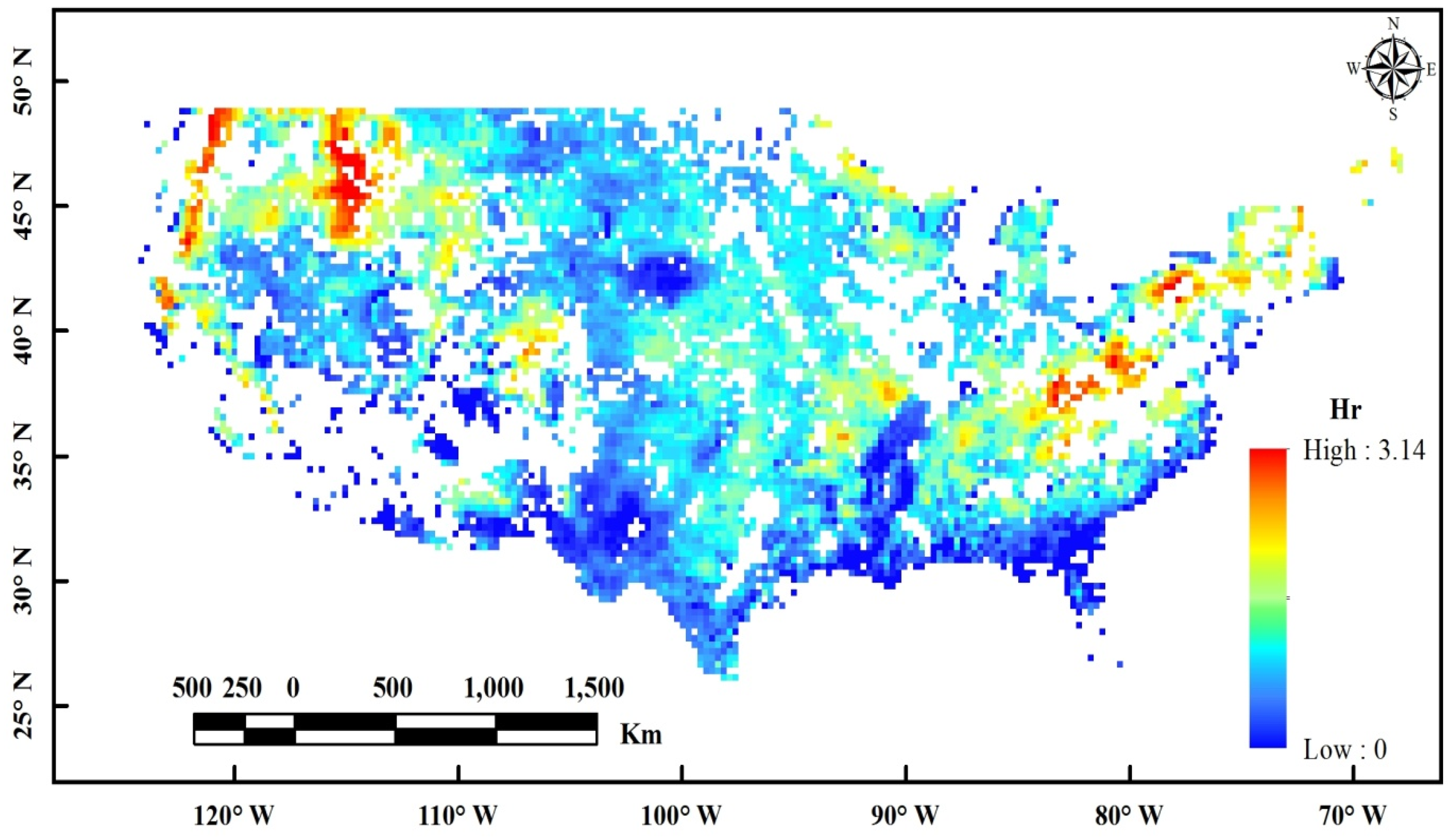
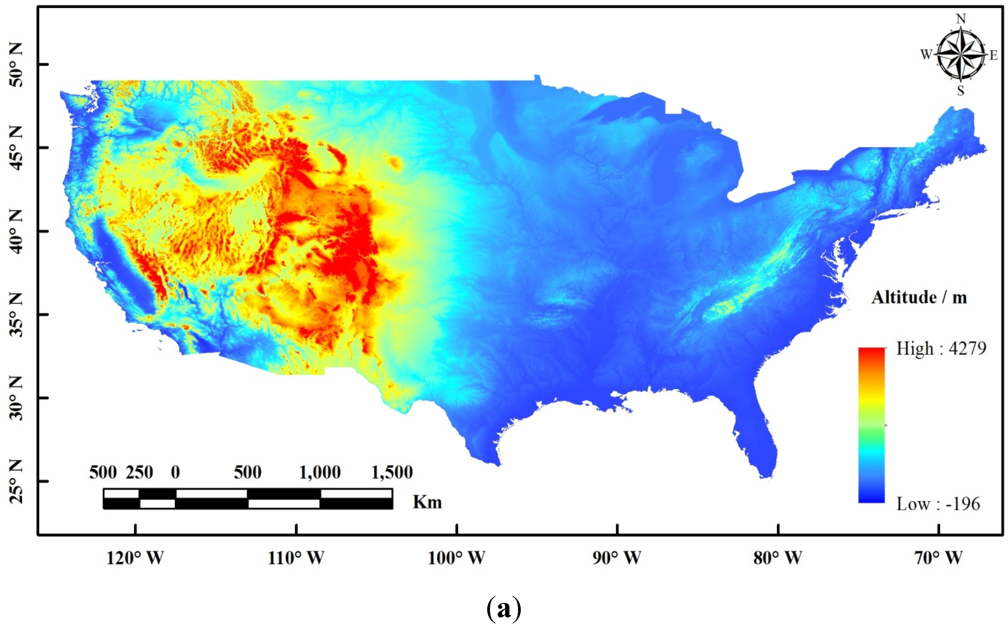
4.3. Maps of Hr Over the USA

For a more concrete illustration of the maps of the Hr parameter, Figure 6 zooms in on the USA from Figure 5 (for the case Q = 0). As the Hr parameter is a synthetic parameter accounting for roughness effects at a large scale, its value may be related to topographic effects. Maps showing the main spatial patterns of topography over the USA are given in terms of altitudes in Figure 7a and slopes in Figure 7b. Even though there is not a perfect match between the spatial patterns given in Figure 6 and in Figure 7a,b, some agreement could be noted in some regions. For instance, it seems the Appalachian Mountains (on the eastern coast), hilly regions in Arkansas and Missouri, and some mountainous regions in the western part of the USA correspond to higher values of the Hr parameter (shown by brighter colors in Figure 6). Similarly, low-altitude and relatively flat regions in the Southern and Central regions of the USA generally correspond to relatively low values of Hr (shown by dark blue colors in Figure 6). Table 3 and Table 4 show the mean values of Hr for the different elevation and slope ranges which corresponded to the nature landforms [66]. It can be seen that the mean values of Hr generally increased with the increase in the elevation (except for the 200–500 m range) and slope. The effect is clearer for the latter parameter which is more directly related to relief: the mean value of Hr increased from about 0.73 to 2.3, when the slope varied from the “nearly level” to the “strongly rolling” classification.

Figure 6. Global map of the retrieved roughness parameter Hr at C-band (AMSR-E observations, January 2010–September 2011), for the case Q = 0 over the USA.

Figure 6. Global map of the retrieved roughness parameter Hr at C-band (AMSR-E observations, January 2010–September 2011), for the case Q = 0 over the USA.

Figure 7. (a) The U.S. topographic map of altitude (1 km spatial resolution) (b) the U.S. topographic map of the slope classification (1 km spatial resolution).

Figure 7. (a) The U.S. topographic map of altitude (1 km spatial resolution) (b) the U.S. topographic map of the slope classification (1 km spatial resolution).

Table 3. Hr values for the different elevation ranges over the United States.

DEM (m)	Classification	Count	Mean Hr
<200	Plain	1080	0.60
200–500	Plateau	2420	0.95
500–1000	Hill	1501	0.78
>1000	Mountain	2730	0.82

Table 3. Hr values for the different elevation ranges over the United States.

DEM (m)	Classification	Count	Mean Hr
<200	Plain	1080	0.60
200–500	Plateau	2420	0.95
500–1000	Hill	1501	0.78
>1000	Mountain	2730	0.82

Table 4. Hr values for the different slope ranges over the United States.

Slope(°)	Classification	Count	Mean Hr
0–2	nearly level	8005	0.73
2–10	undulating	526	1.23
10–15	gently rolling	135	1.42
15–20	moderately rolling	29	1.39
20–25	strongly rolling	8	2.33

Table 4. Hr values for the different slope ranges over the United States.

Slope(°)	Classification	Count	Mean Hr
0–2	nearly level	8005	0.73
2–10	undulating	526	1.23
10–15	gently rolling	135	1.42
15–20	moderately rolling	29	1.39
20–25	strongly rolling	8	2.33

4.4. Sensitivity Analysis

In this section we evaluate the sensitivity of the retrieved values of Hr to the main assumptions made in our modelling approach.

(1) Sensitivity to the value of the Q parameter.

The Q parameter accounts for polarization mixing effects. As noted in Section 3, Montpetit et al. [27] have found that the value Q = 0.075 can be used over a large frequency range and Wang et al. [57] have found values of Q ranging from 0 to 0.3 at C-band. In this sensitivity study, in addition to the case Q = 0, we set the values of the Q parameter to 0.1, 0.2 and 0.3 and we calculated the corresponding Hr values. The results are shown in Figure 8a,b. It can be seen that, for the three cases Q = 0.1, 0.2, and 0.3, similar results were obtained in comparison to the case Q = 0, except that slightly lower values of R² were generally obtained and lower values of the Hr parameter were retrieved systematically. As shown in Figure 8a, the average values of Hr for all the biomes decreased with increasing values of Q: comparing to the case Q = 0, the average values of Hr decreased by values varying between 0.1 (for desert) and 0.8 (for broadleaf deciduous forests, mixed coniferous and high latitude deciduous forests) for the case Q = 0.3. The average values of Hr for the forest biomes decreased more than for the other biomes. Note that because an increase in the value of the Q parameter generally leads to a decrease in the difference between TB_H and TB_V (TB_H increases and TB_V decreases), the parameter a* may become negative when using Equation (3) for the case Q = 0.3. These negative values correspond to non-physical values and were discarded. Therefore, there are fewer data for the case Q = 0.3 in the retrieved values of Hr especially in the desert regions (such as Australia and Sahara desert).

For each biome, there is only a slight change in R² when modifying the values of Q from 0 to 0.3 (Figure 8b). However, the values of R² are always larger for the case Q = 0 and they decrease with increasing values of Q. All these results confirm the fact, noted by Montpetit et al. [27] from experimental data sets, that rather low values of Q are suitable to model the effects of roughness at the frequencies of AMSR-E.

(2) Sensitivity to the vegetation threshold

In the Method section, we defined “vegetated surface” as the pixels where more than 85% of the NDVI values exceed the threshold value of 0.07. To investigate the sensitivity of the Hr values to the value of this vegetation threshold, we made two sets of changes. Firstly, we changed the thresholds of NDVI from 0.07 to 0.05 and 0.1, while keeping the vegetation threshold at 85%. Secondly, we kept the thresholds of NDVI at 0.07 and changed the vegetation threshold from 85% to 80% and 90%.

Figure 8. (a) Sensitivity analysis: influence of the Q parameter (for Q =0, Q = 0.1, Q = 0.2 and Q = 0.3) on the mean values of Hr for a variety of biomes; (b) Sensitivity analysis: influence of theQ parameter (for Q =0, Q = 0.1, Q = 0.2 and Q = 0.3) on the mean R² values of the regression Equation (11) for a variety of biomes.

Figure 8. (a) Sensitivity analysis: influence of the Q parameter (for Q =0, Q = 0.1, Q = 0.2 and Q = 0.3) on the mean values of Hr for a variety of biomes; (b) Sensitivity analysis: influence of theQ parameter (for Q =0, Q = 0.1, Q = 0.2 and Q = 0.3) on the mean R² values of the regression Equation (11) for a variety of biomes.

We found that, as shown in Table 5, there was only a very low percentage of pixels (less than ~ 0.5%) changing categories from “vegetated surface” to “bare or sparsely vegetated surfaces” and therefore there was almost no change in the mean retrieved value of Hr over all the biomes.

Table 5. Percentage of pixels belonging to the categories “Vegetated” and “Bare or Sparsely vegetated” surfaces depending on the NDVI and vegetation threshold.

NDVI Thresholds	Vegetation Threshold	Bare or Sparsely Vegetated Surfaces	Vegetated Surfaces
0.05	85%	23.98%	76.12%
0.07	80%	24.03%	75.97%
	85%	24.03%	75.97%
	90%	24.03%	75.97%
0.1	85%	24.58%	75.42%

Table 5. Percentage of pixels belonging to the categories “Vegetated” and “Bare or Sparsely vegetated” surfaces depending on the NDVI and vegetation threshold.

NDVI Thresholds	Vegetation Threshold	Bare or Sparsely Vegetated Surfaces	Vegetated Surfaces
0.05	85%	23.98%	76.12%
0.07	80%	24.03%	75.97%
	85%	24.03%	75.97%
	90%	24.03%	75.97%
0.1	85%	24.58%	75.42%

(3) Sensitivity to the R² threshold

To evaluate the sensitivity of our results to the used value of the R² threshold for the relationship between a* and NDVI, we conducted a test changing the R² threshold from 0.2 to 0.3. As can be seen in Table 6, the mean values of Hr over the different biomes changed by less than ~0.1. Thus, the main results obtained in this study are still valid using a different value of the R² threshold for the relationship between a* and NDVI.

Table 6. Table 2 using a R² threshold of 0.3, instead of 0.2.

Classification	R2 > 0.3
	Mean Hr	Mean R2	N
Broadleaf evergreen forest	0.95	0.48	1451
Broadleaf deciduous forest & woodland	1.48	0.52	1998
Mixed coniferous & broadleaf deciduous forest & woodland	1.57	0.52	1888
Coniferous forest & woodland	1.33	0.49	3548
High latitude deciduous forest & woodland	1.89	0.50	2888
Wooded & grassland	0.57	0.56	26,043
Shrubs & bare ground	0.37	0.56	3641
Tundra	1.10	0.50	7950
Cultivation	0.72	0.52	20,904
Desert	0.25	--	24,386

Table 6. Table 2 using a R² threshold of 0.3, instead of 0.2.

Classification	R2 > 0.3
	Mean Hr	Mean R2	N
Broadleaf evergreen forest	0.95	0.48	1451
Broadleaf deciduous forest & woodland	1.48	0.52	1998
Mixed coniferous & broadleaf deciduous forest & woodland	1.57	0.52	1888
Coniferous forest & woodland	1.33	0.49	3548
High latitude deciduous forest & woodland	1.89	0.50	2888
Wooded & grassland	0.57	0.56	26,043
Shrubs & bare ground	0.37	0.56	3641
Tundra	1.10	0.50	7950
Cultivation	0.72	0.52	20,904
Desert	0.25	--	24,386

5. Conclusions

A first attempt to compute global maps of the Hr parameter was carried out in this study, based on AMSR-E observations. With the methods described, we attempted to correct for the vegetation effects, and regions classified as broadleaf evergreen forests were masked out. However, it is likely that a larger uncertainty is associated with the retrieved values of Hr for pixels covered by relatively dense vegetation covers and in forested areas. For instance, high Hr values were retrieved in many forested regions, such as in northern Asia and northwestern regions of America, which were mainly covered by evergreen and deciduous coniferous forests, and central and southern regions of China, which were mainly covered by deciduous broadleaf forests. This may be caused by the saturation of the NDVI values over forests, where the linear relationship between NDVI and vegetation optical depth may be not valid. Even though vegetation effects could not be perfectly corrected in densely vegetated regions, it is likely the global map of Hr computed in this study could represent the main spatial patterns of the surface roughness effects in low vegetated regions. We found that clear spatial patterns could be distinguished in the global maps and could be associated with the main cover types (Table 2). It is important to note that the Hr parameter is a complex synthetic parameter which accounts for many effects, such as surface roughness, soil moisture heterogeneities [18,67], vegetation litter in prairies and forests [41,60,67,68], topography [69], etc. These different effects occur over a large domain of spatial scales. This means the interpretation of the obtained global maps of Hr remains difficult. Nevertheless, it seems that higher values of Hr were generally obtained in forested areas. It likely that this result is related to the effects of vegetation, which may not be totally corrected. However, this result may be related also to the effects of litter which are generally taken into account through the Hr parameter. For instance Grant et al. [68] have retrieved values of Hr greater than 0.1 to account for the effects of litter over both a coniferous and a deciduous forest in flat experimental sites. Larger values of Hr were also obtained in hilly regions, as found in the results illustrated for the USA in Section 4. It seems this result confirms the fact that Hr is an effective parameter which may be used to account for the effects of topography in SM retrieval studies at coarse spatial resolution.

All the results presented in this study are sensitive to the assumptions made in our modeling approach. In particular, we found that the global maps of Hr we obtained were sensitive to the value selected for the Q parameter. Retrieved Hr values would significantly decrease if we used a higher Q value such as Q = 0.3. Hence, the maps presented in this study are valid for low values of the Q parameter, which is an assumption often made at C-band [18]. Moreover, a recent study [27] has confirmed the fact that a low value of the Q parameter can be used to model the effects of roughness over a large frequency range. Note also that the use of large values of Q make the decoupling between the roughness and vegetation effects more difficult (lower values were obtained in the R² values of the relationship between a* and NDVI over all types of biomes).

In future studies, we will evaluate whether the global maps of Hr computed in this study have the potential for improving soil moisture retrieval for present and future spaceborne microwave remote sensing missions at the C-band.

References

1. Jackson, T.J., III. Measuring surface soil moisture using passive microwave remote sensing. Hydrol. Process. 1993, 7, 139–152. [Google Scholar]
2. Drusch, M. Initializing numerical weather prediction models with satellite-derived surface soil moisture: Data assimilation experiments with ECMWF’s integrated forecast system and the TMI soil moisture data set. J. Geophys. Res.: Atmos. 2007, 112, D03102. [Google Scholar] [CrossRef]
3. Douville, H.; Chauvin, F. Relevance of soil moisture for seasonal climate predictions: A preliminary study. Clim. Dyn. 2000, 16, 719–736. [Google Scholar] [CrossRef]
4. Njoku, E.G.; Jackson, T.J.; Lakshmi, V.; Chan, T.K.; Nghiem, S.V. Soil moisture retrieval from AMSR-E. IEEE Trans. Geosci. Remote Sens. 2003, 41, 215–229. [Google Scholar] [CrossRef]
5. Wigneron, J.-P.; Schmugge, T.; Chanzy, A.; Calvet, J.-C.; Kerr, Y. Use of passive microwave remote sensing to monitor soil moisture. Agronomie 1998, 18, 27–43. [Google Scholar] [CrossRef]
6. Jackson, T.J.; Gasiewski, A.J.; Oldak, A.; Klein, M.; Njoku, E.G.; Yevgrafov, A.; Christiani, S.; Bindlish, R. Soil moisture retrieval using the C-band polarimetric scanning radiometer during the Southern Great Plains 1999 Experiment. IEEE Trans. Geosci. Remote Sens. 2002, 40, 2151–2161. [Google Scholar] [CrossRef]
7. Njoku, E.G.; Chan, S.K. Vegetation and surface roughness effects on AMSR-E land observations. Remote Sens. Environ. 2006, 100, 190–199. [Google Scholar] [CrossRef]
8. Njoku, E.G.; Entekhabi, D. Passive microwave remote sensing of soil moisture. J. Hydrol. 1996, 184, 101–129. [Google Scholar] [CrossRef]
9. Wigneron, J.P.; Calvet, J.C.; Pellarin, T.; Van de Griend, A.A.; Berger, M.; Ferrazzoli, P. Retrieving near-surface soil moisture from microwave radiometric observations: Current status and future plans. Remote Sens. Environ. 2003, 85, 489–506. [Google Scholar] [CrossRef]
10. Al Bitar, A.; Leroux, D.; Kerr, Y.H.; Merlin, O.; Richaume, P.; Sahoo, A.; Wood, E.F. Evaluation of SMOS soil moisture products over continental U.S. using the SCAN/SNOTEL network. IEEE Trans. Geosci. Remote Sens. 2012, 50, 1572–1586. [Google Scholar]
11. Wigneron, J.P.; Calvet, J.C.; Kerr, Y.; Chanzy, A.; Lopes, A. Microwave emission of vegetation: Sensitivity to leaf characteristics. IEEE Trans. Geosci. Remote Sens. 1993, 31, 716–726. [Google Scholar] [CrossRef]
12. Wigneron, J.-P.; Chanzy, A.; Calvet, J.-C.; Bruguier, N. A simple algorithm to retrieve soil moisture and vegetation biomass using passive microwave measurements over crop fields. Remote Sens. Environ. 1995, 51, 331–341. [Google Scholar] [CrossRef]
13. Bindlish, R.; Jackson, T.J.; Gasiewski, A.J.; Klein, M.; Njoku, E.G. Soil moisture mapping and AMSR-E validation using the PSR in SMEX02. Remote Sens. Environ. 2006, 103, 127–139. [Google Scholar] [CrossRef]
14. Wigneron, J.P.; Parde, M.; Waldteufel, P.; Chanzy, A.; Kerr, Y.; Schmidl, S.; Skou, N. Characterizing the dependence of vegetation model parameters on crop structure, incidence angle, and polarization at L-band. IEEE Trans. Geosci. Remote Sens. 2004, 42, 416–425. [Google Scholar] [CrossRef]
15. Saleh, K.; Wigneron, J.P.; Waldteufel, P.; de Rosnay, P.; Schwank, M.; Calvet, J.C.; Kerr, Y.H. Estimates of surface soil moisture under grass covers using L-band radiometry. Remote Sens. Environ. 2007, 109, 42–53. [Google Scholar] [CrossRef]
16. Al-Yaari, A.; Wigneron, J.P.; Ducharne, A.; Kerr, Y.; de Rosnay, P.; de Jeu, R.; Govind, A.; Al Bitar, A.; Albergel, C.; Muñoz-Sabater, J.; et al. Global-scale evaluation of two satellite-based passive microwave soil moisture datasets (SMOS and AMSR-E) with respect to land data assimilation system estimates. Remote Sens. Environ. 2014, 149, 181–195. [Google Scholar] [CrossRef] [Green Version]
17. Jacquette, E.; Al Bitar, A.; Mialon, A.; Kerr, Y.; Quesney, A.; Cabot, F.; Richaume, P. SMOS CATDS level 3 global products over land. Proc. SPIE 2010, 7824, 375–380. [Google Scholar]
18. Wigneron, J.P.; Laguerre, L.; Kerr, Y.H. A simple parameterization of the L-band microwave emission from rough agricultural soils. IEEE Trans. Geosci. Remote Sens. 2001, 39, 1697–1707. [Google Scholar] [CrossRef]
19. Choudhury, B.J.; Schmugge, T.J.; Chang, A.; Newton, R.W. Effect of surface roughness on the microwave emission from soils. J. Geophys. Res.: Ocean. 1979, 84, 5699–5706. [Google Scholar] [CrossRef]
20. Shi, J.C.; Chen, K.S.; Qin, L.; Jackson, T.J.; O’Neill, P.E.; Leung, T. A parameterized surface reflectivity model and estimation of bare-surface soil moisture with L-band radiometer. IEEE Trans. Geosci. Remote Sens. 2002, 40, 2674–2686. [Google Scholar] [CrossRef]
21. Mialon, A.; Wigneron, J.P.; de Rosnay, P.; Escorihuela, M.J.; Kerr, Y.H. Evaluating the L-MEB model from long-term microwave measurements over a rough field, SMOSREX 2006. IEEE Trans. Geosci. Remote Sens. 2012, 50, 1458–1467. [Google Scholar] [CrossRef] [Green Version]
22. Mo, T.; Choudhury, B.J.; Schmugge, T.J.; Wang, J.R.; Jackson, T.J. A model for microwave emission from vegetation-covered fields. J. Geophys. Res.: Ocean. 1982, 87, 11229–11237. [Google Scholar] [CrossRef]
23. Lawrence, H.; Wigneron, J.P.; Demontoux, F.; Mialon, A.; Kerr, Y.H. Evaluating the semiempirical H-Q model used to calculate the L-band emissivity of a rough bare soil. IEEE Trans. Geosci. Remote Sens. 2013, 51, 4075–4084. [Google Scholar] [CrossRef]
24. Fernandez-Moran, R.; Wigneron, J.P.; Lopez-Baeza, E.; Salgado-Hernanz, P.M.; Mialon, A.; Miernecki, M.; Alyaari, A.; Parrens, M.; Schwank, M.; Wang, S.; et al. Evaluating the impact of roughness in soil moisture and optical thickness retrievals over the VAS area. In Proceedings of 2014 IEEE International Geoscience and Remote Sensing Symposium (IGARSS 2014), 13–18 July 2014; pp. 1947–1950.
25. Wang, J.R.; Choudhury, B.J. Remote sensing of soil moisture content, over bare field at 1.4 GHz frequency. J. Geophys. Res.: Ocean. 1981, 86, 5277–5282. [Google Scholar] [CrossRef]
26. Wigneron, J.P.; Kerr, Y.; Waldteufel, P.; Saleh, K.; Escorihuela, M.J.; Richaume, P.; Ferrazzoli, P.; de Rosnay, P.; Gurney, R.; Calvet, J.C.; et al. L-band microwave emission of the biosphere (L-MEB) model: Description and calibration against experimental data sets over crop fields. Remote Sen. Environ. 2007, 107, 639–655. [Google Scholar] [CrossRef]
27. Montpetit, B.; Royer, A.; Wigneron, J.P.; Chanzy, A.; Mialon, A. Evaluation of multi-frequency bare soil microwave reflectivity models. Remote Sens. Environ. 2015, 162, 186–195. [Google Scholar] [CrossRef]
28. Owe, M.; de Jeu, R.; Holmes, T. Multisensor historical climatology of satellite-derived global land surface moisture. J. Geophys. Res.: Earth Surf. 2008, 113, F01002. [Google Scholar] [CrossRef]
29. Jackson, T.J.; Cosh, M.H.; Bindlish, R.; Starks, P.J.; Bosch, D.D.; Seyfried, M.; Goodrich, D.C.; Moran, M.S.; Jinyang, D. Validation of advanced microwave scanning radiometer soil moisture products. IEEE Trans. Geosci. Remote Sens. 2010, 48, 4256–4272. [Google Scholar] [CrossRef]
30. Kerr, Y.H.; Njoku, E.G. A semiempirical model for interpreting microwave emission from semiarid land surfaces as seen from space. IEEE Trans. Geosci. Remote Sens. 1990, 28, 384–393. [Google Scholar] [CrossRef]
31. Kerr, Y.H.; Waldteufel, P.; Wigneron, J.P.; Martinuzzi, J.; Font, J.; Berger, M. Soil moisture retrieval from space: The soil moisture and Ocean Salinity (SMOS) mission. IEEE Trans. Geosci. Remote Sens. 2001, 39, 1729–1735. [Google Scholar] [CrossRef]
32. Kerr, Y.H.; Waldteufel, P.; Wigneron, J.P.; Delwart, S.; Cabot, F.; Boutin, J.; Escorihuela, M.J.; Font, J.; Reul, N.; Gruhier, C.; et al. The SMOS mission: New tool for monitoring key elements of the global water cycle. Proc. IEEE 2010, 98, 666–687. [Google Scholar] [CrossRef] [Green Version]
33. Kerr, Y.H.; Waldteufel, P.; Richaume, P.; Wigneron, J.P.; Ferrazzoli, P.; Mahmoodi, A.; Al Bitar, A.; Cabot, F.; Gruhier, C.; Juglea, S.E.; et al. The SMOS soil moisture retrieval algorithm. IEEE Trans. Geosci. Remote Sens. 2012, 50, 1384–1403. [Google Scholar] [CrossRef]
34. Al-Yaari, A.; Wigneron, J.P.; Ducharne, A.; Kerr, Y.H.; Wagner, W.; De Lannoy, G.; Reichle, R.; Al Bitar, A.; Dorigo, W.; Richaume, P.; et al. Global-scale comparison of passive (SMOS) and active (ASCAT) satellite based microwave soil moisture retrievals with soil moisture simulations (MERRA-Land). Remote Sens. Environ. 2014, 152, 614–626. [Google Scholar] [CrossRef] [Green Version]
35. Berthon, L.; Mialon, A.; Cabot, F.; Bitar, A.A.; Richaume, P.; Kerr, Y.; Leroux, D.; Bircher, S.; Lawrence, H.; Quesney, A.; et al. CATDS Level 3 DATA Product Description-Soil Moisture and Brightness Temperature Part; CESBIO: Toulouse, France, 2012. [Google Scholar]
36. Kerr, Y.; Waldteufel, P.; Richaume, P.; Ferrazzoli, P.; Wigneron, J.P. Algorithm Theoretical Basis Document (ATBD) for the SMOS Level 2 Soil Moisture Processor; CESBIO: Toulouse, France, 2011. [Google Scholar]
37. Xinxin, L.; Lixin, Z.; Weihermuller, L.; Lingmei, J.; Vereecken, H. Measurement and simulation of topographic effects on passive microwave remote sensing over mountain areas: A case study from the Tibetan Plateau. IEEE Trans. Gesosci. Remote Sens. 2014, 52, 1489–1501. [Google Scholar] [CrossRef]
38. Huete, A.; Justice, C.; Wim, V.L. MODIS Vegetation Index (MOD13). Algorithm Theoretical Basis Document. Available online: http://vip.arizona.edu/documents/MODIS/MODIS_VI_ATBD.pdf (accessed on 1 February 2006).
39. Lawrence, H.; Wigneron, J.-P.; Richaume, P.; Novello, N.; Grant, J.; Mialon, A.; Al Bitar, A.; Merlin, O.; Guyon, D.; Leroux, D.; et al. Comparison between SMOS vegetation optical depth products and MODIS vegetation indices over crop zones of the USA. Remote Sens. Environ. 2014, 140, 396–406. [Google Scholar] [CrossRef]
40. Schaefer, G.L.; Cosh, M.H.; Jackson, T.J. The USDA natural resources conservation service soil climate analysis network (SCAN). J. Atmos. Ocean. Technol. 2007, 24, 2073–2077. [Google Scholar] [CrossRef]
41. Grant, J.P.; Wigneron, J.P.; van de Griend, A.A.; Kruszewski, A.; Søbjærg, S.S.; Skou, N. A field experiment on microwave forest radiometry: L-band signal behaviour for varying conditions of surface wetness. Remote Sens. Environ. 2007, 109, 10–19. [Google Scholar] [CrossRef]
42. Parrens, M.; Wigneron, J.P.; Richaume, P.; Kerr, Y.; Wang, S.; Alyaari, A.; Fernandez-Moran, R.; Mialon, A.; Escorihuela, M.J.; Grant, J.P. Global maps of roughness parameters from L-band SMOS observations. In Proceedings of 2014 IEEE International Geoscience and Remote Sensing Symposium (IGARSS 2014), 13–18 July 2014; pp. 4675–4678.
43. Dirmeyer, P.A.; Gao, X.; Zhao, M.; Guo, Z.; Oki, T.; Hanasaki, N. GSWP-2: Multimodel analysis and implications for our perception of the land surface. Bull. Am. Meteorol. Soc. USA 2006, 87, 1381–1397. [Google Scholar] [CrossRef]
44. Fao, F. UNESCO Soil Map of the World; World Resources Report; ISRIC: Wageningen, The Netherlands, 1988; p. 138. [Google Scholar]
45. Verdin, K.L.; Jenson, S. Development of continental scale DEMs and extraction of hydrographic features. In Proceedings of the Third International Conference/Workshop on Integrating GIS and Environmental Modeling, Santa Fe, NM, USA, 21–25 January 1996.
46. Njoku, E.G.; Ashcroft, P.; Chan, T.K.; Li, L. Global survey and statistics of radio-frequency interference in AMSR-E land observations. IEEE Trans. Geosci. Remote Sens. 2005, 43, 938–947. [Google Scholar] [CrossRef]
47. Oliva, R.; Daganzo, E.; Kerr, Y.H.; Mecklenburg, S.; Nieto, S.; Richaume, P.; Gruhier, C. SMOS Radio frequency interference scenario: Status and actions taken to improve the RFI environment in the 1400-1427-MHz passive band. IEEE Trans. Geosci. Remote Sens. 2012, 50, 1427–1439. [Google Scholar] [CrossRef] [Green Version]
48. Li, L.; Njoku, E.; Im, E.; Chang, P.; St.Germain, K. A preliminary survey of radio-frequency interference over the U.S. in Aqua AMSR-E data. IEEE Trans. Geosci. Remote Sens. 2004, 42, 380–390. [Google Scholar] [CrossRef]
49. Skou, N.; Misra, S.; Balling, J.E.; Kristensen, S.S.; Sobjaerg, S.S. L-Band RFI as experienced during airborne campaigns in preparation for SMOS. IEEE Trans. Geosci. Remote Sens. 2010, 48, 1398–1407. [Google Scholar] [CrossRef]
50. Draper, C.; Mahfouf, J.F.; Calvet, J.C.; Martin, E.; Wagner, W. Assimilation of ASCAT near-surface soil moisture into the SIM hydrological model over France. Hydrol. Earth Syst. Sci. 2011, 15, 3829–3841. [Google Scholar] [CrossRef] [Green Version]
51. Mladenova, I.E.; Jackson, T.J.; Njoku, E.; Bindlish, R.; Chan, S.; Cosh, M.H.; Holmes, T.R.H.; de Jeu, R.A.M.; Jones, L.; Kimball, J.; et al. Remote monitoring of soil moisture using passive microwave-based techniques—Theoretical basis and overview of selected algorithms for AMSR-E. Remote Sens. Environ. 2014, 144, 197–213. [Google Scholar] [CrossRef]
52. Van de Griend, A.A.; Owe, M. Microwave vegetation optical depth and inverse modelling of soil emissivity using Nimbus/SMMR satellite observations. Meteorl. Atmos. Phys. 1994, 54, 225–239. [Google Scholar]
53. Kurum, M. Quantifying scattering albedo in microwave emission of vegetated terrain. Remote Sens. Environ. 2013, 129, 66–74. [Google Scholar] [CrossRef]
54. Jackson, T.J.; ASCE, A.M. Profile soil moisture from surface measurements. J. Irrig. Drain. Div. 1980, 106, 81–92. [Google Scholar]
55. Wang, S.; Wigneron, J.P.; Parrens, M.; Al-Yaari, A.; Fernandez-Moran, R.; Jiang, L.M.; Zeng, J.Y.; Kerr, Y. Evaluating roughness effects on C-band AMSR-E observations. In Proceedings of 2014 IEEE International Geoscience and Remote Sensing Symposium (IGARSS 2014), 13–18 July 2014; pp. 3311–3314.
56. Martens, B.; Lievens, H.; Walker, J.; Panciera, R.; Tanase, M.; Monerris, A.; Gao, Y.; Wu, X.L.; Verhoest, N. An alternative roughness parameterization for soil moisture retrievals from passive microwave observations. In Proceedings of the 2013 ESA Living Planet Symposium, Edinburgh, UK, 9–13 September 2013.
57. Wang, J.R.; O’Neill, P.E.; Jackson, T.J.; Engman, E.T. Multifrequency measurements of the effects of soil moisture, soil texture, and surface roughness. IEEE Trans. Geosci. Remote Sens. 1983, GE-21, 44–51. [Google Scholar] [CrossRef]
58. Owe, M.; de Jeu, R.; Walker, J. A methodology for surface soil moisture and vegetation optical depth retrieval using the microwave polarization difference index. IEEE Trans. Geosci. Remote Sens. 2001, 39, 1643–1654. [Google Scholar] [CrossRef]
59. Schmugge, T.; Jackson, T.J.; Kustas, W.P.; Wang, J.R. Passive microwave remote sensing of soil moisture: Results from HAPEX, FIFE and MONSOON 90. ISPRS J. Photogramm. Remote Sens. 1992, 47, 127–143. [Google Scholar] [CrossRef]
60. Semi-empirical regressions at L-band applied to surface soil moisture retrievals over grass. Remote Sens. Environ. 2006, 101, 415–426. [CrossRef]
61. Zeng, J.Y.; Li, Z.; Chen, Q.; Bi, H.Y. A simplified physically-based algorithm for surface soil moisture retrieval using AMSR-E data. Front. Earth Sci. 2014, 8, 427–438. [Google Scholar] [CrossRef]
62. Jones, M.O.; Jones, L.A.; Kimball, J.S.; McDonald, K.C. Satellite passive microwave remote sensing for monitoring global land surface phenology. Remote Sens. Environ. 2011, 115, 1102–1114. [Google Scholar] [CrossRef]
63. Liu, Y.Y.; de Jeu, R.A.M.; McCabe, M.F.; Evans, J.P.; van Dijk, A.I.J.M. Global long-term passive microwave satellite-based retrievals of vegetation optical depth. Geophys. Res. Lett. 2011, 38, L18402. [Google Scholar]
64. Montandon, L.M.; Small, E.E. The impact of soil reflectance on the quantification of the green vegetation fraction from NDVI. Remote Sens. Environ. 2008, 112, 1835–1845. [Google Scholar] [CrossRef]
65. Wigneron, J.P.; Kerr, Y.; Waldteufel, P.; Ferrazzoli, P.; Richaume, P.; Saleh, K.; Calvet, J.-C.; Chanzy, A. Recent advances in modelling the land surface emission at L-band-application to L-MEB in the operational SMOS algorithm. In Proceedings of 2nd International Symposium on Recent Advances in Quantitative Remote Sensing (RAQRS’II 2006), Torrent (Valencia), Spain, 15 October 2006.
66. Su, S.; Li, J. Geomorphologic Mapping; Surveying and Mapping Press: Beijing, China, 1999. [Google Scholar]
67. Mo, T.; Schmugge, T.J. A parameterization of the effect of surface roughness on microwave emission. IEEE Trans. Geosci. Remote Sens. 1987, GE-25, 481–486. [Google Scholar] [CrossRef]
68. Grant, J.P.; Saleh-Contell, K.; Wigneron, J.P.; Guglielmetti, M.; Kerr, Y.H.; Schwank, M.; Skou, N.; Van de Griend, A.A. Calibration of the L-MEB model over a coniferous and a deciduous forest. IEEE Trans. Geosci. Remote Sens. 2008, 46, 808–818. [Google Scholar] [CrossRef]
69. Mialon, A.; Coret, L.; Kerr, Y.H.; Secherre, F.; Wigneron, J.P. Flagging the topographic impact on the SMOS signal. IEEE Trans. Geosci. Remote Sens. 2008, 46, 689–694. [Google Scholar] [CrossRef] [Green Version]