Classification of Vessels in Single-Pol COSMO-SkyMed Images Based on Statistical and Structural Features

Abstract

Vessel monitoring is one of the most important maritime applications of Synthetic Aperture Radar (SAR) data. Because of the dihedral reflections between the vessel hull and sea surface and the trihedral reflections among superstructures, vessels usually have strong backscattering in SAR images. Furthermore, in high-resolution SAR images, detailed information on vessel structures can be observed, allowing for vessel classification in high-resolution SAR images. This paper focuses on the feature analysis of merchant vessels, including bulk carriers, container ships and oil tankers, in 3 m resolution COSMO-SkyMed stripmap HIMAGE mode images and proposes a method for vessel classification. After preprocessing, a feature vector is estimated by calculating the average value of the kernel density estimation, three structural features and the mean backscattering coefficient. Support vector machine (SVM) classifier is used for the vessel classification, and the results are compared with traditional methods, such as the K-nearest neighbor algorithm (K-NN) and minimum distance classifier (MDC). In situ investigations are conducted during the SAR data acquisition. Corresponding Automatic Identification System (AIS) reports are also obtained as ground truth to evaluate the effectiveness of the classifier. The preliminary results show that the combination of the average value of the kernel density estimation and mean backscattering coefficient has good ability for classifying the three types of vessels. When adding the three structural features, the results slightly improve. The result of the SVM classifier is better than that of K-NN and MDC. However, the SVM requires more time, when the parameters of the kernel are estimated.

1. Introduction

Vessel classification is of increasing interest to many fields, such as marine environmental monitoring, fishing law-enforcement, and maritime traffic monitoring. Synthetic aperture radar (SAR) is an active sensor that has a powerful surveillance capability, allowing for observations regardless of the weather conditions, time of day, or cooperation of the vessel. Furthermore, the available satellite SAR systems operating in L-, C- and X-band offer products with various swaths and spatial resolutions. Because of these characteristics and flexibility, SAR remote sensing is one of the most important technologies for vessel monitoring at sea.

For nearly thirty years, vessel detection has been popular in SAR applications. Much progress has been achieved in vessel detection using SAR technology [1,2]. Vessel detection can provide information on vessel positions. If a user wants to determine the vessel type, vessel classification is needed [3,4]. Compare with vessel detection, few studies have been conducted on vessel classification. The initial attempts at vessel classification were mainly based on inverse synthetic aperture radar (ISAR) vessel images [5,6,7] and backscattering simulation images of vessels [8,9]. Recently, polarimetric SAR data have also been exploited for vessel classification [10,11]. In addition to using ISAR data and PolSAR data, some studies on single-polarization real SAR images, such as ENVISAT-ASAR and ERS images, have been conducted. In the project of detection and classification of marine traffic from space (DECLIMS), Greidanus et al. demonstrated that output of vessel classification based on ERS-2, ENVISAT-ASAR Image and Alternate polarization modes, RADARSAT-1 Standard and Fine modes SAR images was only limited to size estimates [12]. Margarit et al. presented a vessel classification algorithm based on fuzzy logic. Experimental results based on the ENVISAT-ASAR and ERS data at a resolution of approximately 30 meters showed that the preliminary percentage of positive classifications was approximately 70% [3,13]. In medium resolution SAR images (30 to 10 m), energy scattered from different parts of a vessel usually overlap in a few pixels. No additional details on the vessel structure can be found. Thus, it is difficult to discriminate vessel types based on those images alone. For vessel classification, high-resolution images (10 to 3 m), in which details increase, are needed.

Fortunately, with the launch of advanced SAR satellites, such as COSMO-SkyMed, TerraSAR-X and Radarsat-2, whose image resolutions are as high as 3 m, it has become possible to observe more vessel structural features in SAR images and classify vessels. Knapskog et al. [14] analyzed characteristics of ships in TerraSAR-X and airborne SAR images, and proposed a vessel classification method. In their work, silhouettes of vessels extracted from steep incidence angle SAR images were compared with silhouettes of 3-D models to discriminate vessels with comparable sizes and shapes [4]. Teutsch et al. [15] presented an approach for segmentation and classification of man-made objects in TerraSAR-X images. Chen Wen-ting et al. [16] proposed a novel two-stage feature selection approach for ship classification in TerraSAR-X images. Xing [17] proposed a method based on the sparse representation in feature space for classification in TerraSAR-X images. Jiang [18,19] used structural features to classify civilian vessels in COSMO-SkyMed images. Zhang [20] and Wang [21] analyzed the scattering components of ships in COSMO-SkyMed images to represent the superstructure of different ship types, and classified ships into three types: bulk carriers, container ships and oil tankers.

Although the previous studies achieved encouraging results, vessel classification is still an issue. In high-resolution SAR images, vessels are detailed; the characteristics of an object are different from those in a medium resolution image. Therefore, the features and method should be improved for new data.

In this paper, we propose a merchant vessel classification methodology based on feature analysis in high-resolution SAR images. Bulk carriers, container ships and oil tankers are three types of mainstream merchant ships of the international shipping market. Therefore vessels in the SAR images are classified into those three categories.

Based on image characteristic analyses of the three types of vessels, the average value of kernel density estimation, three structural features, mean backscattering coefficient, local radar cross section density and the ratio of width and length are investigated for distinguishing the three classes of vessels. The selected features are input to the classifier. A support vector machine (SVM) classifier is used for the ship classification and is compared with the traditional methods, such as K-nearest neighbor algorithm (K-NN) [22] and minimum distance classifier (MDC) [22] to evaluate the classification results. Experiments are performed with 3 m COSMO-SkyMed stripmap HIMAGE mode products. Vessel information acquired from in situ investigations and Automatic Identification System (AIS) reports is used as the ground truth for the analysis and evaluation.

The paper is organized as follows. Section 2 provides the algorithm assumption for the vessel classification in the paper. Section 3 describes the characteristics of bulk carriers, container ships, and oil tankers in high-resolution SAR images. Section 4 introduces the data processing chain, including image preprocessing, scattering and structural features extraction and the classifier. Section 5 presents the classification experiment results and analysis of the classification model selection, the feature analyses and a comparison with other methods. Finally, the conclusions are presented in Section 6.

2. Algorithm Assumption

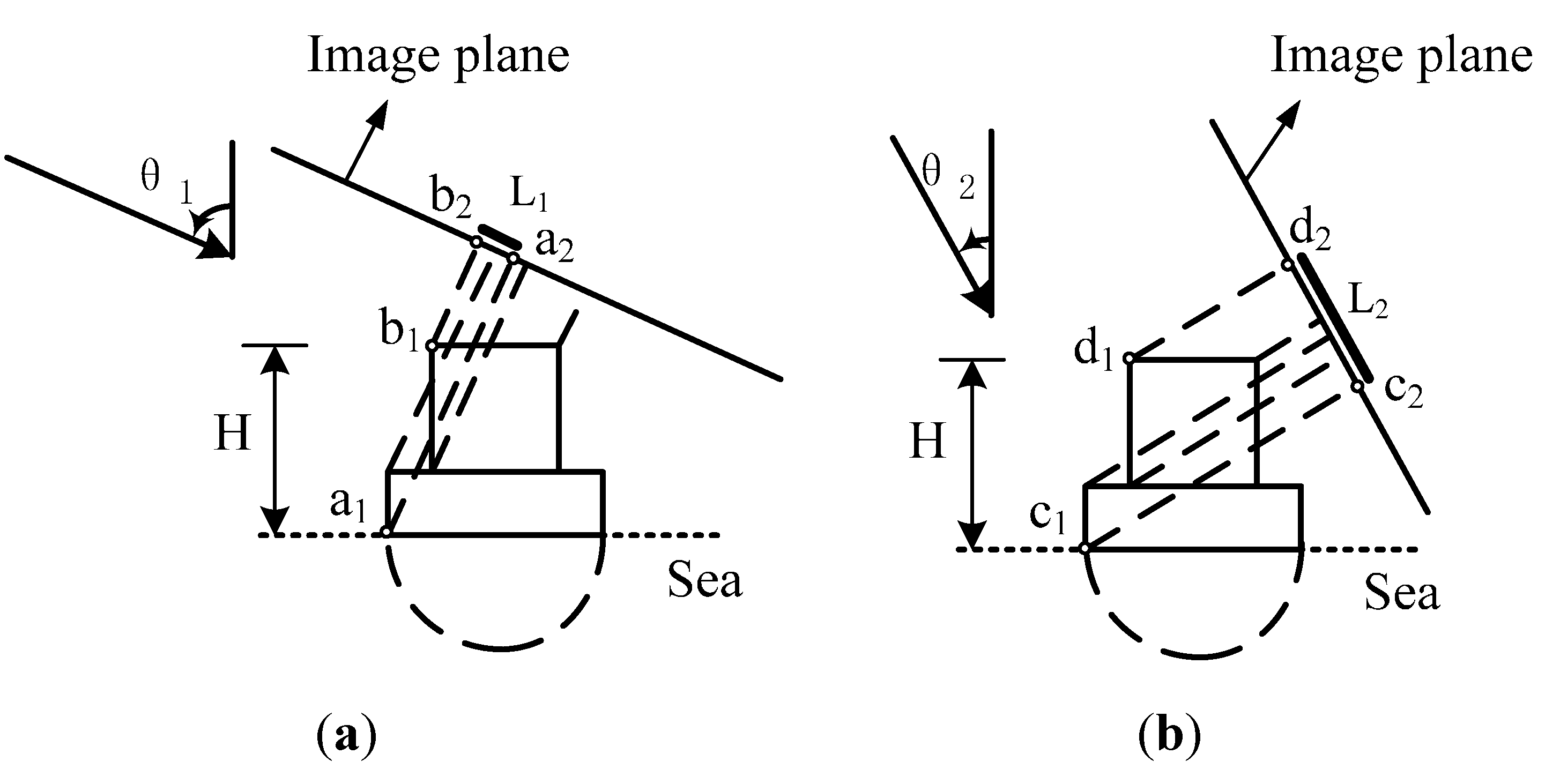
Based on the analyses of simulated polarimetric images, Margarit [9] suggested that at steep incidence angles, e.g., 15°–35°, the scattering response of a vessel seems stable along a frequency and ship bearing. In this case, superstructures of a vessel are usually stretched out in high-resolution SAR images due to layover. Equation (1) expresses the relation among the layover L in the slant range, the object height H and the incidence angle of a radar wave θ. According to (1), assuming that H is known, the value of L is shorter as θ (0° < θ < 90°) increases.

$$L=H\cdot \cos (\theta )$$

(1)

Figure 1 illustrates the imaging geometry of a vessel in a SAR image at different incidence angles. θ_i (i = 1,2) are the incidence angles of a radar wave. H is the height of the vessel above the sea surface. L_i (i = 1,2) are lengths of the layover in SAR image. Equation (1) and Figure 1 show that steep incidence angle lead to considerable layover (Figure 1b) for tall objects, such as the superstructure of a ship, while shallow incidence angle leads to small layover (Figure 1a).

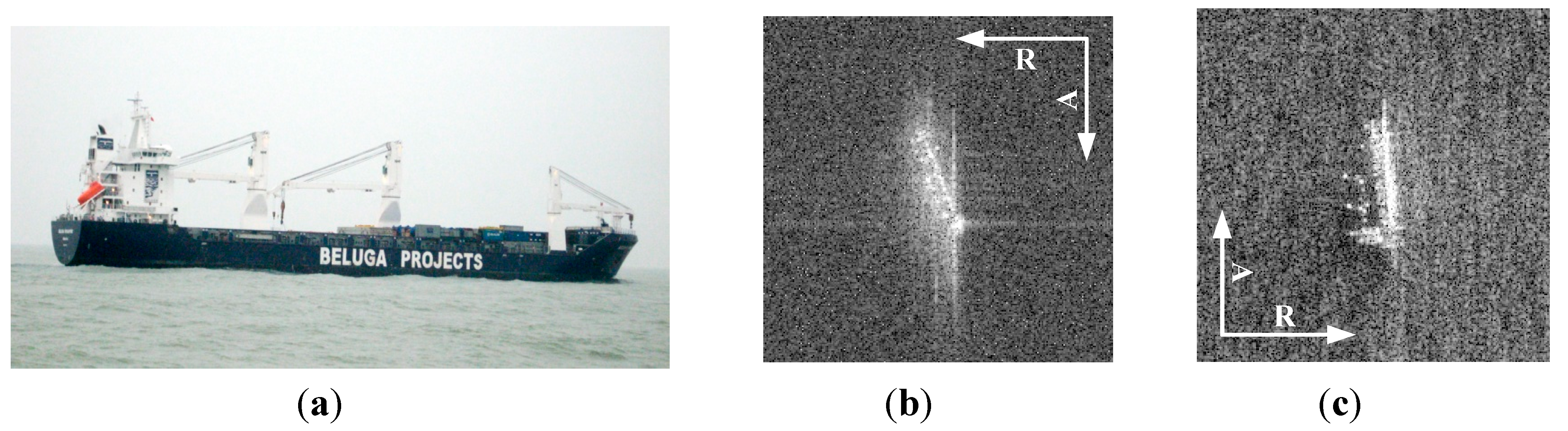
Figure 2 is an example of a container ship in a COSMO-SkyMed 3 m resolution SAR image at different incidence angles. According to the AIS information, the container ship named BELUGA has a length of 162 m and a width of 33 m. Figure 2a is the in situ photograph. Figure 2b,c shows the same ship in the SAR images at 9:33 am and 10:21 am respectively, of the same day in 2010. According to the position of the ships in the image and the metadata of the image, the local incidence angles at the ship positions can be calculated. In this case, the incidence angle of Figure 2b is approximately 59.0º and that of Figure 2c is approximately 26.4°. We can see that considerable layover occurs in the steep incidence angle image. In this case, the silhouette of the vessel can be used as a feature for vessel classification [4]. For a shallow incidence angle, the images show apparent top-view projections of the ships [14], and the structures on the decks are relatively apparent. Scattering from the superstructure above the deck is significant. In a sense, the locations of the strong scatters are related physical structures of the vessel. Therefore, the features can be used for vessel classification.

Figure 1. Layover of a vessel at different incidence angles. (a) is a shallow incidence angle; and (b) is a steep incidence angle.

Figure 1. Layover of a vessel at different incidence angles. (a) is a shallow incidence angle; and (b) is a steep incidence angle.

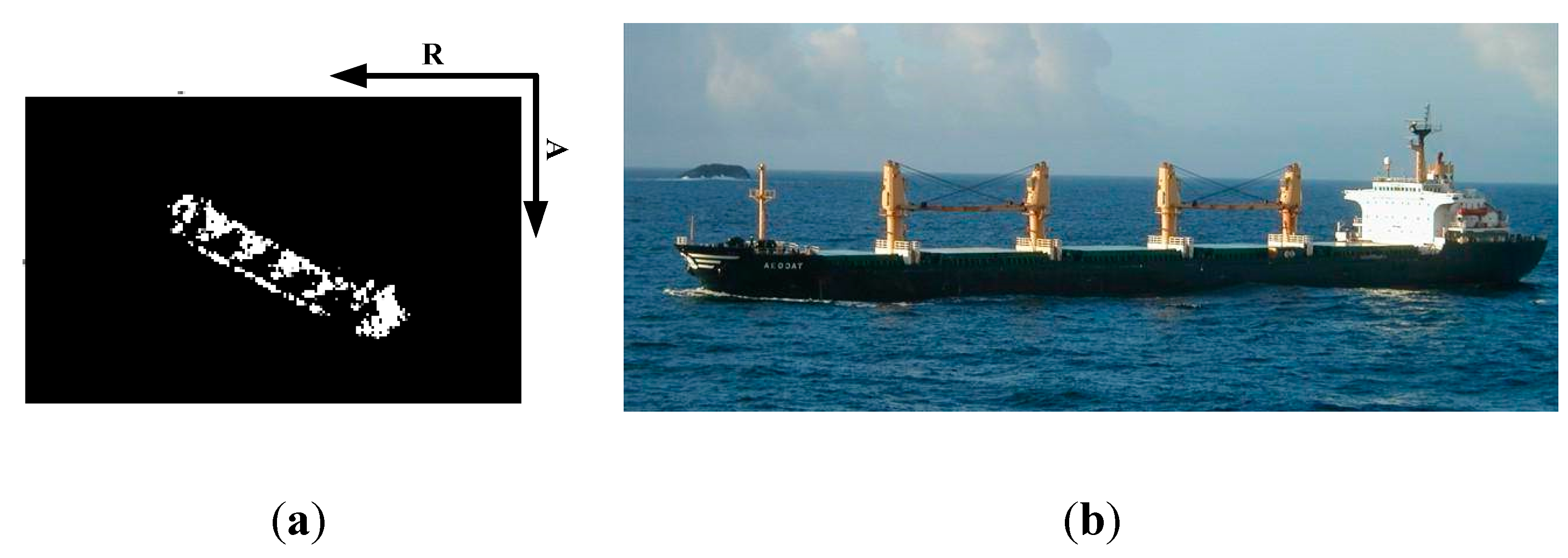
Figure 2. An example of a container ship in a SAR image at different incidence angles; (a) an in situ photo; (b) shallow incidence angle of 59.0°; and (c) steep incidence angle of 26.4°. (A is the azimuth direction, and R is the range direction).

Figure 2. An example of a container ship in a SAR image at different incidence angles; (a) an in situ photo; (b) shallow incidence angle of 59.0°; and (c) steep incidence angle of 26.4°. (A is the azimuth direction, and R is the range direction).

It is known, the movement along the azimuth coordinate of a vessel usually leads to blurring in the SAR image. It is difficult to extract effective features from a smeared image for vessel classification. Therefore, for simplicity, only anchored vessels in the image are considered. In addition, small ships cannot show detail structures in the image, so the merchant ships over 150 m long are considered for the experiments.

Therefore, in this paper, we focus on moored and large vessel classification in high-resolution SAR images at shallow incidence angles according to the integrated features and present an improved processing chain.

3. Scattering Characteristics of Vessels in High-Resolution SAR Images

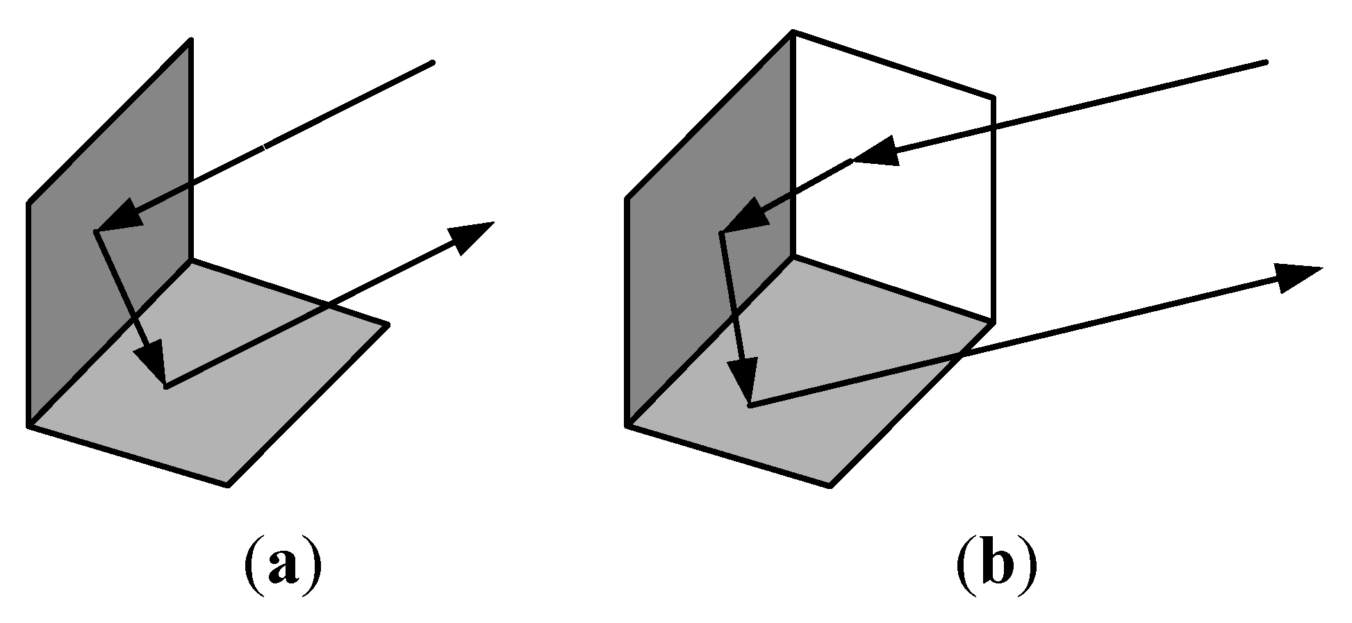
Dihedral or trihedral reflectors reflect most radar energy back to the sensor when they face the radar beam (Figure 3). Therefore, the reflectors are usually bright in SAR image. Because of the dihedral reflections between the vessel hull and sea surface and trihedral reflections among the superstructures on the deck, vessels usually give strong backscattering in SAR image. The backscattering depends on several properties, such as the structure of the ship, the orientation of the ship relative to the sensor, the material, the motion, and the SAR system parameters [20]. Generally, the flat deck and other slightly curved plates produce strong specular reflection when viewed at off-nadir directions, so very low backscattering is received by radar; these areas appear dark in the SAR image. However, the superstructure and the ancillary facilities, such as the funnel, deckhouse, arm of the crane, and goods (e.g., containers), which are usually composed of metal, form dihedral or trihedral reflectors and become the dominant scatterers in the images. Notably, the deckhouse usually has apparent sidelobes along the range and azimuth directions, because of the strong backscattering due to the dihedral or trihedral structure formed by the walls of the cabin and deck. In some situations the main-mast also shows strong backscattering in a SAR image [9]. Moreover, a large dihedral reflector made up of the water surface and the hull side, which faces the radar, also has considerable backscattering that is seen as a bright line in SAR images. The locations of strong scatterers and weak backscattering regions in an image are usually related to the physical structures of the vessel. Bulk carriers, container ships and oil tankers have unique physical structure. Therefore, the distributions of backscattering in the SAR image are also different for the three categories of vessels. 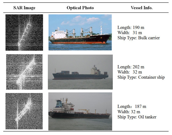Table 1 demonstrates the three types of vessels. The SAR images are sub-scenes from 3 m resolution X-band COSMO-SkyMed stripmap HIMAGE images.

Figure 3. Examples of a dihedral reflector (a); and a trihedral reflector (b).

Figure 3. Examples of a dihedral reflector (a); and a trihedral reflector (b).

A bulk carrier usually has large box-like hatches on its deck. The hatched edges and the main deck form a dihedral reflector, which produces strong echo signals. However, the flat hatches often transmit specular reflection. As a result, bulk carriers show up as bright stripes with light and dark intervals. The bright stripes have the same width as the hatch, and they are perpendicular to the ship’s side. The side of the ship’s hull toward the incident direction has a clear boundary. The other hull side, in contrast, has a relatively weak echo (Table 1, top).

For a container ship, the rectangular containers loaded on the deck, which are composed of metallic materials, have strong reflections because of the corner reflectors formed by them. So, the container ships transmit strong echoes overall. If the container is fully loaded, then the entire hull appears as a bright spot. If the containers are placed randomly, we can obtain irregularly strong echo signals. Compared with the bulk carriers, container ships have more intensive spots and the distribution of the strong scatterers in the SAR image is more irregular (Table 1, middle).

Oil tankers have a flat deck. In the middle of the deck, there are oil pipelines from the stern to the bow. The facilities are usually symmetric along the oil pipeline. Generally, the pipeline and the facilities are composed of metallic materials that form a large number of dihedral and even trihedral reflectors. Thus, there is usually a distinct backscattering line in the middle of oil tankers (Table 1, bottom).

Table 1. Examples and optical photos of a bulk carrier, container ship and oil tanker in SAR image (the azimuth direction of the SAR image is from bottom to top, and the range direction of the SAR image is from left to right. The local incidence angles of the image from top to bottom are approximately 50.3°, 50.54°, and 50.53°, respectively).

SAR Image	Optical Photo	Vessel Info.
		Length: 190 m Width: 31 m Ship Type: Bulk carrier
		Length: 202 m Width: 32 m Ship Type: Container ship
		Length: 187 m Width: 32 m Ship Type: Oil tanker

Table 1. Examples and optical photos of a bulk carrier, container ship and oil tanker in SAR image (the azimuth direction of the SAR image is from bottom to top, and the range direction of the SAR image is from left to right. The local incidence angles of the image from top to bottom are approximately 50.3°, 50.54°, and 50.53°, respectively).

SAR Image	Optical Photo	Vessel Info.
		Length: 190 m Width: 31 m Ship Type: Bulk carrier
		Length: 202 m Width: 32 m Ship Type: Container ship
		Length: 187 m Width: 32 m Ship Type: Oil tanker

4. Methodology

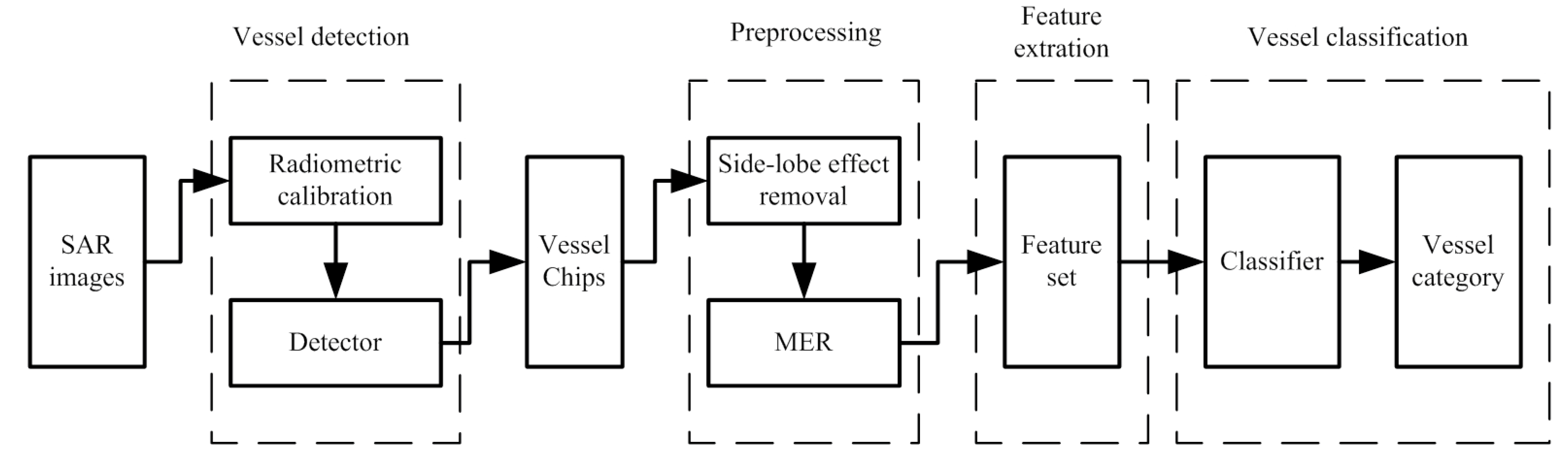
The flowchart of our method for classifying vessel types is shown in Figure 4. First, radiometric calibration of the data is performed by the Next ESA SAR Toolbox (NEST) for the quantitative analysis. A feature based constant false alarm rate (CFAR) detector [23] is employed to help us locate vessel candidates in the image. However, it is impossible for one method to detect all true vessels without any false alarms or errors. Therefore, the vessel candidates are refined by manually interpreting with AIS information after the vessel detection. Then, for improved vessel classification, the regions of interest, which are image sub-scenes that contain one vessel each, are extracted. The major work of the vessel classification in the paper is based on the well-identified and isolated chips. Before the classification, the chips undergo pre-processing, which includes side-lobe effect reduction and minimum enclosing rectangle (MER) extraction. The features are extracted from the vessel pixels in the MER to avoid negative effects from the sea backscattering for statistical analysis. Lastly, the vessels are classified into different categories based on the features.

Figure 4. Flowchart of the vessel classification in a SAR image.

Figure 4. Flowchart of the vessel classification in a SAR image.

4.1. Preprocessing

The band-limited characteristics of SAR systems together with the slight oversampling can cause that the contribution of a single target extends to more than a single cell. The point-spread function (PSF), which is basically a bi-dimensional sinc, will present redundant information around the main lobe and visible side lobes when high-power scatterers are placed in areas with a limited coefficient of backscattering [24]. Ships usually have strong backscattering due to their metallic materials and superstructure. Generally, the metallic deckhouses, containers and other superstructures may produce bright lines along the range or azimuth direction, due to the side-lobe effect. In this paper, a side-lobe reduction method in the image domain is applied [21].

MER is a signature dimension box containing a vessel and is defined as the smallest rectangle that contains major pixels of a vessel. In this paper, all feature extractions are based on the MER. So, the MER is directly related to the accuracy of the recognition of merchant ships.

The bearing of the vessel or orientation angle α ρelative to the vertical or azimuth direction (which is north in each SAR image) is estimated via the order moment as suggested in [21]:

$$\alpha =\frac{1}{2}{\tan }^{-1}\left(\frac{2{\mu }_{11}}{{\mu }_{20}-{\mu }_{02}}\right)+\frac{\pi }{2}B$$

(2)

μ_pq is defined by Equation (3).

$${\mu }_{pq}={\displaystyle \sum _x{\displaystyle \sum _y{(x-\overline{x})}^p{(y-\overline{y})}^q}}f(x,y)(p=0,1,2\begin{array}{c};\end{array}q=0,1,2)$$

(3)

where f(x,y) is the pixel value at (x,y). $\left(\overline{x, }\overline{y}\right)$ is the centroid of a chip and is defined as $\overline{x }$ $=\raisebox{1ex}{$m_{10}$}\!\left/ \!\raisebox{-1ex}{$m_{00}$}\right.$, $\overline{y }=\raisebox{1ex}{$m_{01}$}\!\left/ \!\raisebox{-1ex}{$m_{00}.$}\right.$m_pq is the (p+q) order moment and is defined as m_pq = ∑∑x^py^pf(x,y). B is the π/2 mbiguity of the orientation. When μ₂₀ > μ₀₂, B = 1; otherwise B = 0

With the orientation angle and centroid, the vessel chips are rotated in vertical direction to ease the application of the MER. Features can also be more easily to be extracted. The MER extraction is based on the binary segmentation image of a vessel (Figure 5).

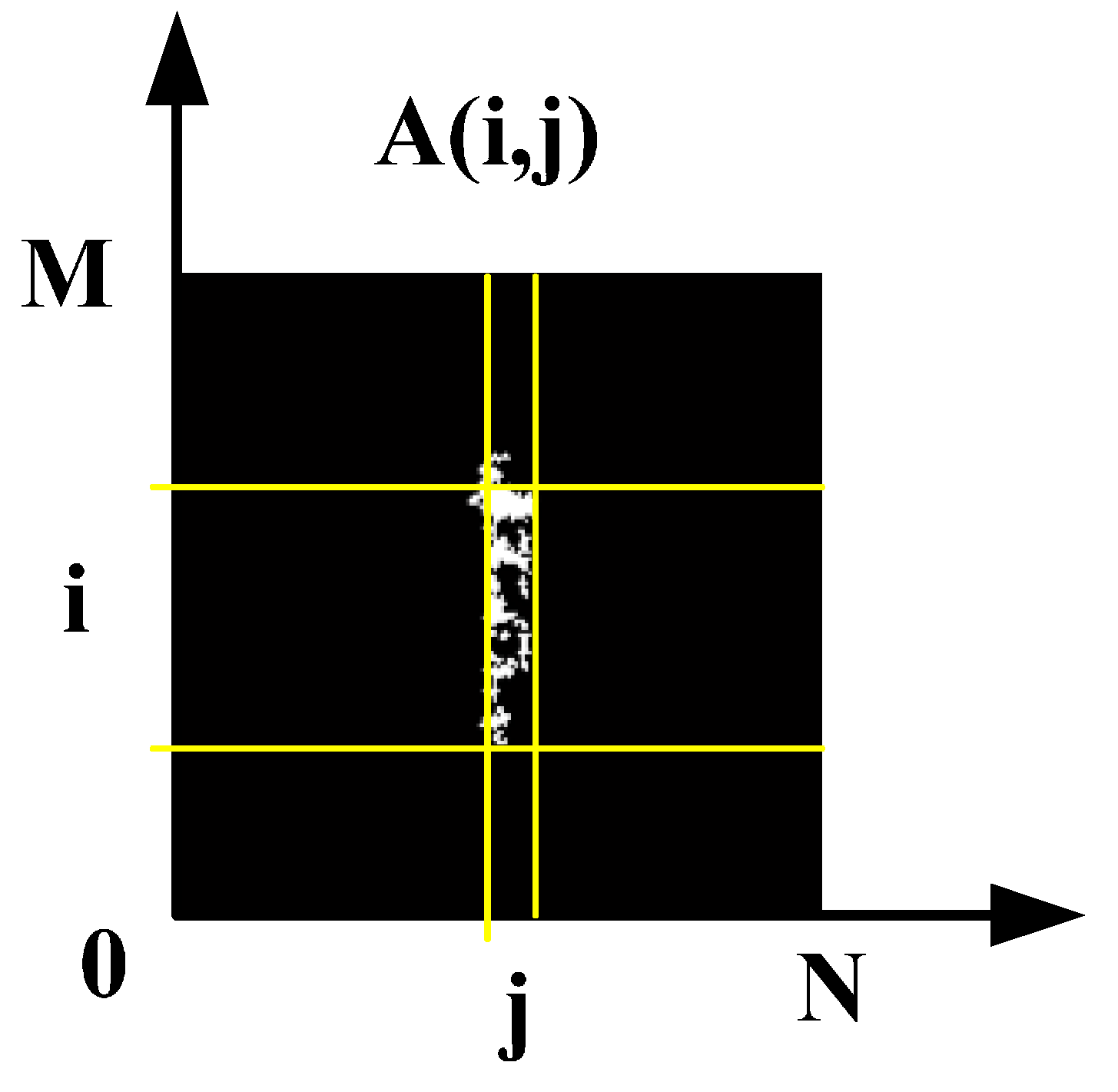
After data calibration, the values of the backscatter coefficient of pixels can be analyzed quantitatively and can be compared image to image. Based on the analysis of the pixel value of the vessels in COSMO-SkyMed SAR images, an empirical threshold of 2 dB is set to segment the vessels in the chip image. If the pixel value is larger than 2 dB, then it will be labeled as 1; otherwise it will be labeled as 0. After the segmentation, a morphological operation is applied to remove small isolated pixels. Thus, the strong backscattering pixel set of the vessel in a chip is obtained, assuming the segment image is A(i, j). Algorithm 1 shows the procedure for the extraction of the left and right boundaries of the MER in the pixel set. Similarly, the top and bottom boundaries can be estimated using ${\text{H}}_{row}\left(i\right)={\displaystyle \sum }_{j=1}^{N}A \left(i,j\right),$ 1≤ i ≤ M. Because the top and bottom boundaries are short, the empirical threshold T is set to 3.

Algorithm 1 finding left and right boundaries of MER

Input: histogram of the segmentation chip. ${\text{H}}_{col}\left(j\right)={\displaystyle \sum }_{i=1}^{M}A \left(i,j\right),$ 1 ≤ j ≤ N. Output: left and right boundaries of MER. set the threshold T = 7 for j = 1 to N, do   Tl = Hcol(j + 1) − Hcol (j)   if Tl≥ T then stop loop    b1 = j, and b1 is left boundary.   end if   else    j = j + 1. continue the loop   end end for for j = N to 1, do   Tr = Hcol (N − j) − Hcol (N − j − 1)   if Tr≥ T then stop loop.    br = j, and br is the right boundary  end if   else    j = j − 1. continue the loop   end end for

Figure 5. MER extraction of a vessel

Figure 5. MER extraction of a vessel

4.2. Feature Set for Classification

After pre-processing the binary pixel extraction, the removal of the side-lobe effect and the MER extraction, the vessel chips are ready for structural feature analysis. We investigate features to describe the structure of a vessel in high-resolution SAR images.

4.2.1. Average Value of Kernel Density Estimation

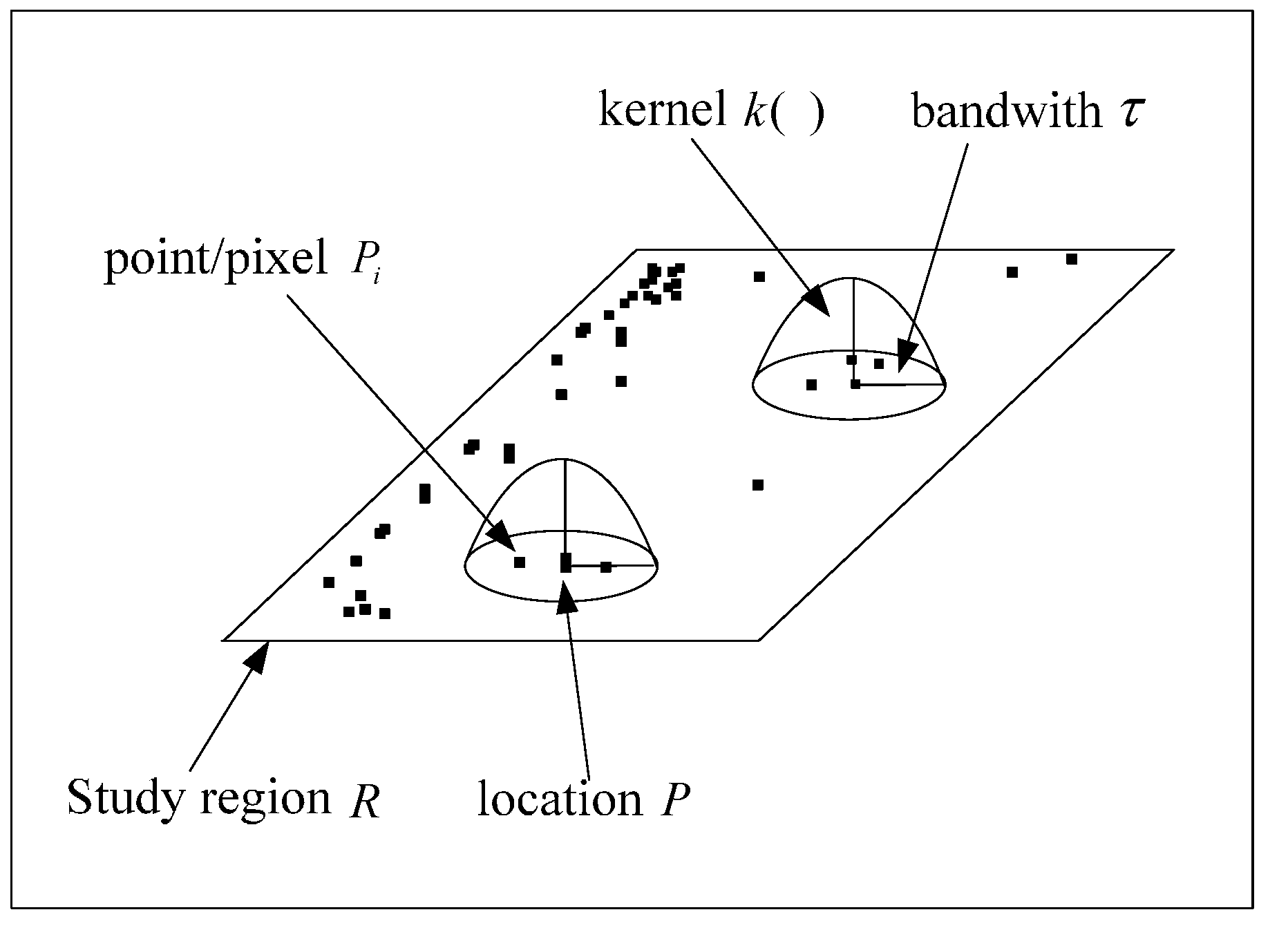
The kernel density estimation (KDE) is one of the nonparametric density estimation methods in the field of point pattern analysis and is an important data analysis tool for determining the structure and distribution of a point dataset. The KDE function allows one to estimate the intensity of a point pattern and to represent it by means of a smoothed three-dimensional continuous surface that represents the variation of density of point events across the study region R [25]. In an image, pixels can be regarded as points. Thus, the KDE can indicate the density of the selected pixel with the relationship between a pixel and its neighbors.

The general form of a kernel estimator is [25]:

$$f(P)={\displaystyle \sum _{i=1}^n\frac{1}{{\tau }^2}}k\left(\frac{P-P_i}{\tau }\right)$$

(4)

where f(P) is the estimate of the density of the spatial point pattern measured at location P, P_i is the observed i^th point, k( ) represents the kernel weighting function and τ is the bandwidth. The value of τ is chosen to provide the required degree of smoothing in the estimate (Figure 6).

Kernel estimation is a generalization of this concept, in which the window is replaced with a moving three-dimensional function (the kernel) that weights events or points within its sphere of influence according to their distance from the point at which the intensity is being estimated. The method is commonly used in a more general statistical context to obtain smooth estimates of univariate (or multivariate) probability densities from an observed sample of observations ([26,27]).

Figure 6. Kernel estimation of a point pattern (re-edited from [26])

Figure 6. Kernel estimation of a point pattern (re-edited from [26])

In our method, a typical kernel called a quartic kernel is chosen. Thus, the estimate of the density distribution f(P) is expressed as Equation (5) [26].

$$f(P)={{\displaystyle \sum _{d_i\le \tau }\frac{3}{\pi {\tau }^2}\left(1-\frac{d_i^2}{{\tau }^2}\right)}}^2$$

(5)

where d_i is the distance between pixel P(x,y) and the other pixels belonging to the same vessel, and the summation only occurs over values of d_i  that do not exceed τ. The region of influence within which the observed points contribute to f(P) is a the circle of radius τ centered on P(x,y). Analysis of the KDE is based on vessel pixels in the MER. After segmentation, a binary image is obtained. In the binary image, only the strong pixels (labeled “1”) are preserved. Those pixels can be regarded as the points in Figure 6. Using Equation (5), we can obtain the KDE value of each pixel.

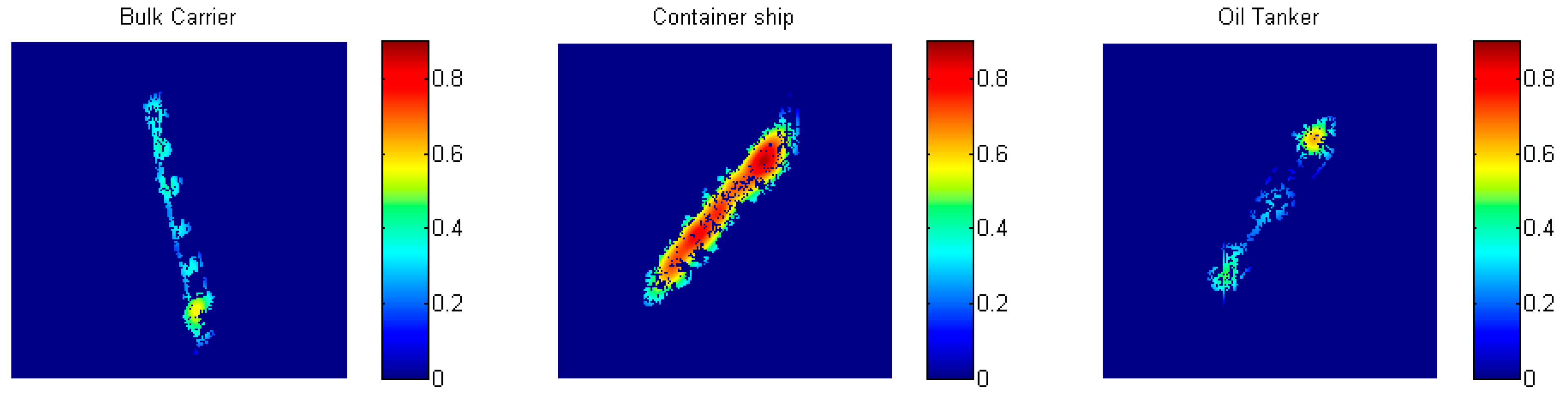
Figure 7. Kernel density estimation of the three types of ships

Figure 7. Kernel density estimation of the three types of ships

Figure 7 shows examples of the performance of the KDE. The first column is the bulk carrier. The second column is the container ship, and the third column is the oil tanker. Container ships have a high density. Usually, a container ship is completely loaded with containers, so it has the largest number of large dihedral and trihedral reflectors; stronger scattering can be found in the image. Bulk carriers and oil tankers also have many dihedral and trihedral reflectors, but they are small and might not add up to a strong signal. The metallic deckhouses are the major strong scatterers. The other facilities, such as pipelines and cranes, spread separately. Therefore, bulk carriers and oil tankers have a relatively low KDE value. To form the feature vector, the average value of the KDE is calculated by Equation (6), in which n denotes the number of vessel pixels.

$$K=\frac{1}{n}{\displaystyle \sum _{i=1}^{n}f(P)}$$

(6)

4.2.2. Features Based on Structural Descriptions

Three features, including the left-right ratio, the ratio of the maximum and middle axes, and the ratio of the maximum and minimum axes, are used to describe the structure of the vessels.

The longest axes (LA) of the vessel in the image, which has the maximum cumulative value along the direction of the ship’s hull or along the vertical direction after the vessel rotation in the preprocessing, is the longest line segment of a ship. A vessel binary image inside the MER, which is rotated and segmented in the processing phase, is B(i,j). Then, the histogram, which is populated by the number of non-zero pixels along the vertical direction in the MER, can be given as:

$$h(j)={\displaystyle \sum _{i=1}^{BM}B(i,j)}\text{ , }1\le j\le BN,B(i,j)>0$$

(7)

The column number J, J = argmax h(j) , is the location of the LA. BM is the length of the MER, and BN is the width of the MER.

Figure 8 provides examples of the three types of vessels. The first column shows examples of the original vessel chips of the three ship categories: a bulk carrier, a container ship, and an oil tanker from top to bottom. The second column is the ship chips after the image rotation and segmentation. The green rectangles and red lines are the MERs and LAs of the ships, respectively. The corresponding histograms (h(j)) along the vertical direction are shown in the third column, where some parameters of the features are also shown in the graph. In Figure 8c,f,i, the horizontal axis denotes the width of the ship. The y-axis denotes h(j), the number of non-zero pixels of the segmented ship in the SAR image within the MER along the vertical, i.e., parallel to the left or right MER border. h_max and h_min are maximum and minimum values of h(j). h_max gives the LA. h_c is h(j) at center of the width. D₁ and D₂ are the two breadths divided by the LA. Therefore, the three features can be defined as follows.

Figure 8. Structural features. A and R are the azimuth and range directions, respectively. (a) original SAR image of a bulk carrier, (b) vessel chip after rotation and segmentation, (c) illustration of structural features, (d) original SAR image of a container ship, (e) vessel chip after rotation and segmentation, (f) illustration of structural features, (g) original SAR image of a oil tanker, (h) vessel chip after rotation and segmentation, and (i) illustration of structural features. The incidence angles of (a), (d), and (g) are approximately 50.32°, 59.49°, 50.22°, respectively.

Figure 8. Structural features. A and R are the azimuth and range directions, respectively. (a) original SAR image of a bulk carrier, (b) vessel chip after rotation and segmentation, (c) illustration of structural features, (d) original SAR image of a container ship, (e) vessel chip after rotation and segmentation, (f) illustration of structural features, (g) original SAR image of a oil tanker, (h) vessel chip after rotation and segmentation, and (i) illustration of structural features. The incidence angles of (a), (d), and (g) are approximately 50.32°, 59.49°, 50.22°, respectively.

Left-Right Ratio (R₁)

For bulk carriers, the LA is usually the ship side facing the radar’s incident wave. The LA is one of the two sides of the ship’s hull. For container ships, the LA is often located around the middle axis. For oil tankers, the main axis is usually the pipeline and the symmetric line. So, the LA is generally also in the center of the ship’s deck. The location of the LA can be characterized by the left-right ratio, which can be defined by Equation (8). To avoid the influence of the boundary, the boundary pixels are not considered when the parameter is calculated.

$$R_1=\frac{\max \{D_1,D_2\}}{\min \{D_1,D_2\}}$$

(8)

where D₁ and D₂ are the distances from the maximum axis to both sides of the MER. According to the definition, container ships and oil tankers usually have a relatively smaller R₁, which is often close to 1, while bulk carriers usually have a larger R₁.

Ratio of Maximum and Middle Axes (R₂)

Assume that the cumulative value along the ship length is h(j), where1< j < BN. R₂ is defined by Equation (9). To avoid the influence of the boundary, the boundary pixels are not considered when the parameter is calculated.

$$R_2=\frac{\max (h(j))}{h_c}=\frac{h_{\max }}{h_c}$$

(9)

where h_max is the maximum value of the histogram, as indicated by the longest blue line in Figure 8c,f,i. h_c denotes the number of positive pixels mid-axis, i.e., at the center of the MER. This parameter allows distinguishing between symmetrical and asymmetrical ship signatures; hence, it is another way to discriminate between container ships, oil tankers and bulk carriers.

Ratio of the Maximum and Minimum Axes (R₃)

R3 is defined by Euation (10), where h_max is the same as mentioned above. h_min is the minimum value of the histogram h(j). In Figure 8c,f,i, the shortest blue line indicates h_min. To avoid the influence of the boundary, the boundary pixels are not considered when the parameter is calculated.

$$R_3=\frac{\max (h(j))}{\min (h(j))}=\frac{h_{\max }}{h_{\min }}$$

(10)

Based on an analysis of Section 3 and Figure 8, the parameter R₃ of a container ship is expected to be small and close to 1, and the R₃ of the bulk carrier is expected to be larger than that of the oil tanker.

4.2.3. Mean Backscattering Coefficient (M)

The mean value is calculated based on the ship pixels after calibration in the range of the MER (Equation (11)). The pixel values of the ship are converted to sigma value σ_ij after the calibration. Pixels with σ_ij > 2dB are selected for statistics to avoid the effect of the background. Thus, the ship’s mean backscattering coefficient is

$$M=\frac{1}{BN\times BM}{\displaystyle \sum {\sigma }_{ij}}({\sigma }_{i,j}>0,1<i<BM,1<j<BN)$$

(11)

M is expected to be largest for a container ship, because there are more strong scatterers on the deck. While bulk carrier and oil tanker have lower mean values.

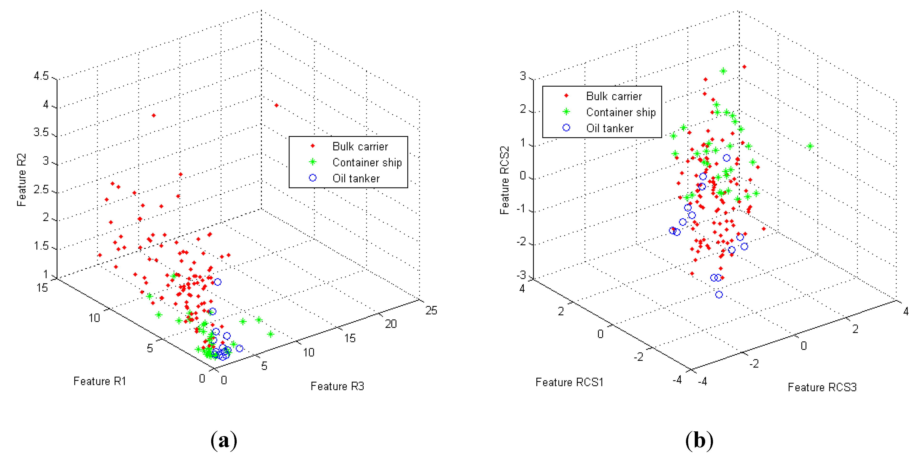
4.2.4. Local Radar Cross Section Density (RCS)

The local RCS density is a typical scattering feature for describing the electromagnetic scattering characteristic of a target in a SAR image [3,17]. For classification, a ship is divided into several parts (usually the bow, middle and stern sections). The local radar cross-section density is the mean RCS value retrieved for the three parts of the ship signature (RCS₁, RCS₂, RCS₃), which are normalized by the maximum value (Equation (12)).

$$RC{S}_i=\frac{M_i/C_i}{\underset{1\le i\le 3}{\max }(M_i/C_i)} i=1,2,3$$

(12)

where M_i and C_i are the total intensity and area of part I, respectively. The local physical structures of different types of ships are distinct due to their functionality. Therefore, the backscattering intensities will differ for the local physical structures of different types of ships.

4.2.5. The Ratio of the Width and Length (RWL)

The ratio of the width and length is usually applied to describe geometric features of a ship [17]. In the paper, the RWL is used for comparing other features.

4.3. Classifier

Support vector machine (SVM) is a supervised learning model with associated learning algorithms that analyze data and recognize patterns on the basis of the structural risk minimization principle in statistics. SVMs have been used for object classification and recognition in high-resolution SAR images [15,17]. A large number of experiments have shown that, compared with traditional neural networks, a SVM has a simpler structure, and better performance, particularly regarding its generalization ability. In addition, SVMs are very useful for solving problems with small sample sets and large dimension. Specifically, the model used in this paper is the C-support vector classification (C-SVC), which was proposed by Boser et al. and was realized by Chih-Chung Chang and Chih-Jen Lin [28].

5. Experiments and Analysis

5.1. Dataset

High-resolution SAR images are acquired for vessel classification. Corresponding AIS data and in situ investigation information are regarded as ground truth for the result identification and analysis.

5.1.1. SAR Data

Four COSMO-SkyMed SAR images of the East China Sea (Figure 9) are acquired for the research. The acquisition time of the data is 12–13 July 2010. The incidence angles of the images are relatively large. Table 2 lists the detailed information on the images. The data are level 1A stripmap HIMAGE products (Single-look Complex Slant (SCS) product).

Figure 9. Map of the data.

Figure 9. Map of the data.

Table 2. Detailed image information.

Satellite	Polarization	Orbit	Acquisition Time	Sample Spacing(m)		Incidence Angle (°)	Look Side	Size
				Range	Azimuth			Samples × Lines
CSKS2	HH	Descending	2010-7-12 09:33:39	1.903	2.234	59.3	right	13874 × 19790
CSKS2	VV	Ascending	2010-7-12 21:59:02	1.666	2.045	49.6	right	18292 × 22886
CSKS3	HH	Descending	2010-7-13 09:33:37	1.903	2.234	59.3	right	17512 × 19790
CSKS3	HH	Ascending	2010-7-13 21:59:00	1.666	2.045	49.6	right	18292 × 22886

Table 2. Detailed image information.

Satellite	Polarization	Orbit	Acquisition Time	Sample Spacing(m)		Incidence Angle (°)	Look Side	Size
				Range	Azimuth			Samples × Lines
CSKS2	HH	Descending	2010-7-12 09:33:39	1.903	2.234	59.3	right	13874 × 19790
CSKS2	VV	Ascending	2010-7-12 21:59:02	1.666	2.045	49.6	right	18292 × 22886
CSKS3	HH	Descending	2010-7-13 09:33:37	1.903	2.234	59.3	right	17512 × 19790
CSKS3	HH	Ascending	2010-7-13 21:59:00	1.666	2.045	49.6	right	18292 × 22886

5.1.2. Validation Data

On 12–19 July 2010, we conducted a field investigation during the SAR satellite passage. The fishery law enforcement ship (No. 206) of the Fishery Law Enforcement Bureau of the East China Sea Region cruised through the experiment area to collect ship names, ship types, in situ photographs, GPS positions, sea states, and so on. However, because of the large coverage of the image, not all vessels in the area could be recorded. Thus, AIS polls were also obtained for the results validation.

AIS systems are designed primarily for maritime safety and particularly for collision avoidance [29]. The system is usually equipped on ships to inform each other about their position, course, speed, name and other parameters of a specific ship. AIS polls from ships are usually collected by coastal receivers. The AIS data we used were obtained by coastal receivers of the Shanghai Maritime Bureau. To correlate the AIS and SAR positions, the acquired AIS messages were received starting before and ending after the SAR image acquisition time. The geolocation of a pixel can be derived based on a Range-Doppler model of a SAR image. So, the AIS and SAR positions can be correlated based on the geo-coordinates. With the AIS messages, information on a ship’s MMSI number, name, call sign, type, position, course, speed, width, length and other parameters can be provided. The information is used as ground truth data to verify the detection results and facilitate feature analysis of ships in the SAR images.

5.2. Experiments and Analysis

After the CFAR detection of ship targets and identification with ground truth data, 158 ship chips are obtained: 110 bulk carriers, 32 container ships, and 16 oil tankers. Half of the dataset is used for training, and the rest is used for testing.

5.2.1. Model and parameter selection of the classifier

SVM is originally designed for binary classification. The “one-against-one” method in LIBSVM (a library for support vector machines) based on C-SVC [30] is adopted for multi-class classification in this paper. Feature vector {K, R₁, R₂, R₃, M} is designed to input to the classifier. The values of the five features lie within different dynamic ranges. However, features with large values may have a greater influence on the cost function than features with small values. Therefore, before applying the SVM, scaling or normalization of the data should be performed to avoid the domination of features in greater numeric ranges over those in smaller numeric ranges and to avoid numerical difficulties during the calculation [31]. A technique normalized by the respective estimates of the mean and variance is adopted [22]. For N available data of a specific feature, x is

$$x\prime =\frac{x_i-\overline{x}}{\sigma },i=1,2,\mathrm{...},N$$

(13)

where $x_i^{\prime }$ is the normalized value. $\overline{x}$ and σ are the mean value and standard deviation, respectively. Then, we obtain the normalized features with a zero mean and unit variance.

For a SVM, the four basic functions of linear, polynomial, radial basis function (RBF) and sigmoid kernel are often used as kernel functions. As suggested in [31], the RBF kernel nonlinearly maps samples into a higher dimensional space. The kernel can handle nonlinear relation between class labels and features. Furthermore, the RBF kernel has less hyperparameters and fewer numerical difficulties than a polynomial kernel. Therefore, the RBF model is selected as the kernel for the classification.

There are two parameters for an RBF kernel: C and γ. To predict the testing data accurately, the two parameters should be strategically selected. In the paper, five-fold cross-validation is conducted to identify good (C,γ) values [31]. The training set is first divided into five subsets of equal size. Sequentially one subset is tested using the classifier trained for the remaining four subsets. Thus, each instance of the entire training set is predicted once such that the cross-validation accuracy is the percentage of data correctly classified. The procedure can prevent the overfitting problem. A “grid search” strategy is conducted for searching the (C,γ) [31]. Half of the samples of each class are selected for training. Exponentially growing sequences of C and γ are used for the grid search. Figure 10 provides the results. In the experiment, the best cross-validation accuracy is 93.7%. One of the best log₂(C) and log₂(γ) , whose value are 0 and −2, are selected. Therefore, in this case, the best (C,γ) is (2⁰,2⁻²). Using the best (C,γ) , the entire training set is trained again to generate the final classifier model.

Figure 10. Grid search for C and γ.

Figure 10. Grid search for C and γ.

5.2.2. Feature Analysis

In this study, the features of Section 4.2 are tested for vessel classification. These features are the KDE average value (K), the left-right ratio (R₁), the ratio of the maximum and middle axes (R₂), the ratio of the maximum and minimum axes (R₃), the mean backscattering coefficient (M), the local radar cross section density (RCS₁, RCS₂, RCS₃) and the ratio of width and length (RWL). Six feature vectors are investigated for the analysis: FV1 = {K, R₁, R₂, R₃, M}, FV2 = {K, RCS₁, RCS₂, RCS₃, M}, FV3 = {RWL, RCS₁, RCS₂, RCS₃, M}, FV4 = {K, M}, FV5 = {R₁, R₂, R₃}, and FV6 = {RCS₁, RCS₂, RCS₃}.

Half of the samples of each class are selected for training and testing. We randomly select the samples for training and conduct the classification experiments 300 times and average the results. Table 3 and Table 4 list the classification results by inputting the feature vectors FV1, FV2, FV3, FV4, FV5 and FV6. The results of the classification with FV1 generally outperform the classification with other feature vectors. The bulk carrier receives a 90% classification accuracy regardless of which feature vector is used. The rates for the container ship and oil tanker fluctuate with the feature vectors. If the local RCS density features are substituted for the structure features (R_1, R_2, R₃), namely, using FV2 instead of FV1, the positive classification rate of the oil tanker decreases from 85.9% to 75.0%. However, the positive classification rate of the container ship increases from 76.3% to 79.6%. If the RWL is substituted for K in FV2, namely, FV3, then the classification rate of the container ship and oil tanker decreases below 25%. Thus, feature K is important for classification, particularly for bulk carriers, which are classified as good with FV1, FV2 and FV4. FV4 is a combination of feature M and K. Based on FV4, the classifier can obtain a high accuracy that is only slightly lower than FV1. If only using structure features (FV5 = {R₁, R₂, R₃}) or scattering features (FV6 = {RCS₁, RCS₂, RCS₃}), the classification rates are not satisfactory (see Table 4).

Table 3. Classification results of the different feature vectors (FV1, FV2, FV3) (BU = bulk carrier, CO = container ship, TA = Oil tanker).

Type	Classification
	FV1 = {K, R1, R2, R3, M}			FV2 = {K, RCS1, RCS2, RCS3, M}			FV3 = {RWL, RCS1, RCS2, RCS3, M}
	BU	CO	TA	BU	CO	TA	BU	CO	TA
BU	97.6%	2.2%	0.2%	97.5%	2.1%	0.4%	90.5%	6.9%	2.6%
CO	14.8%	76.3%	8.9%	17.1%	79.6%	3.3%	74.1%	24.3%	1.6%
TA	7.3%	6.8%	85.9%	12.4%	12.6%	75.0%	72.7%	5.0%	22.3%

Table 3. Classification results of the different feature vectors (FV1, FV2, FV3) (BU = bulk carrier, CO = container ship, TA = Oil tanker).

Type	Classification
	FV1 = {K, R1, R2, R3, M}			FV2 = {K, RCS1, RCS2, RCS3, M}			FV3 = {RWL, RCS1, RCS2, RCS3, M}
	BU	CO	TA	BU	CO	TA	BU	CO	TA
BU	97.6%	2.2%	0.2%	97.5%	2.1%	0.4%	90.5%	6.9%	2.6%
CO	14.8%	76.3%	8.9%	17.1%	79.6%	3.3%	74.1%	24.3%	1.6%
TA	7.3%	6.8%	85.9%	12.4%	12.6%	75.0%	72.7%	5.0%	22.3%

Table 4. Classification results of the different feature vectors (FV4, FV5, FV6) (BU = bulk carrier, CO = container ship, TA = Oil tanker).

Type	Classification
	FV4 = {K, M}			FV5 = {R1, R2, R3}			FV6 = {RCS1, RCS2, RCS3}
	BU	CO	TA	BU	CO	TA	BU	CO	TA
BU	97.4%	2.4%	0.2%	90.8%	7.4%	1.8%	94.9%	3.6%	1.5%
CO	16.5%	75.6%	7.9%	47.6%	43.4%	9.0%	90.1%	9.5%	0.4%
TA	6.6%	8.6%	84.8%	28.0%	27.5%	44.5%	89.8%	1.2%	9.0%

Table 4. Classification results of the different feature vectors (FV4, FV5, FV6) (BU = bulk carrier, CO = container ship, TA = Oil tanker).

Type	Classification
	FV4 = {K, M}			FV5 = {R1, R2, R3}			FV6 = {RCS1, RCS2, RCS3}
	BU	CO	TA	BU	CO	TA	BU	CO	TA
BU	97.4%	2.4%	0.2%	90.8%	7.4%	1.8%	94.9%	3.6%	1.5%
CO	16.5%	75.6%	7.9%	47.6%	43.4%	9.0%	90.1%	9.5%	0.4%
TA	6.6%	8.6%	84.8%	28.0%	27.5%	44.5%	89.8%	1.2%	9.0%

Figure 11 is the plot of the data with a combination of features M and K, i.e., FV4. Most of the bulk carrier K values are below 0.4, while most K values of the container ship are above 0.4. The oil tanker has moderate values of K and relatively small M values. The plot shows that the three types of ships can be reasonably separated based on the combination of features K and M. The classification results in Table 3 and Table 4 are proof.

Figure 11. Plot of the data with a combination of features M and K.

Figure 11. Plot of the data with a combination of features M and K.

Figure 12 is the plot of the data with a combination of features R₁, R₂ and R₃ (FV5) and features RCS_1, RCS₂ and RCS₃ (FV6). The feature vector FV5 can lea d to better class separation than the feature vector FV6. The analysis is consistent with the results in Table 3 and Table 4.

Figure 12. Plot of the data with a combination of (a) features R₁, R₂ and R₃, and (b) features RCS_1, RCS₂ and RCS₃

Figure 12. Plot of the data with a combination of (a) features R₁, R₂ and R₃, and (b) features RCS_1, RCS₂ and RCS₃

In summary, feature K is important for the classification. The classifier based on the combination of features K and M can lead to good classification results. When adding features R₁, R₂ and R₃, the classification results improved slightly. However, features R₁, R₂ and R₃ can describe the difference in structures of the different vessels. Thus, the feature vector FV1 = {K, R₁, R₂, R₃, M} is recommended as input for the classifier.

5.2.3. Classification Results Analysis

To evaluate the performance of the method, half of the samples of each class are selected for training and testing. Because of the limited number of samples, we randomly select the samples for training and conduct repeated classification experiments and average the results. The feature vector FV1 = {K, R₁, R₂, R₃, M} is the input for the vessel classification. Figure 13 illustrates the average classification results at different times. The red, green and blue lines are the classification results of the bulk carrier, container ship and oil tanker, respectively. The pink line is the overall ratio of the positive classification. When the classification exceeds approximately 100 iterations (only 50 for the BU), a further increase in the number of classification does not improve the results. After 100 classification iterations, the average ratios of the positive classification are close to 98%, 76% and 86% of the bulk carrier, container ship and oil tanker, respectively. The ratio of the positive classification reaches 92%.

Figure 13. Classification results.

Figure 13. Classification results.

The positive classification rate is highest for the bulk carrier. As mentioned above, the most significant features of a bulk carrier in the high-resolution SAR image is the repetitive pattern in the longitudinal direction. Except for the deckhouse and flat hatches, there are few superstructures on the deck of a bulk carrier. Therefore, the features of the bulk carrier are relatively stable in the image. Although there are some cranes on the deck of some bulk carriers, the image retains the pattern well. Figure 14 is an example of a bulk carrier with a crane, the incidence angle of the image is approximately 50°. A large oil tanker usually shows symmetry along its centerline in a SAR image. Besides the deckhouse and main pipeline, other pipelines and pumping systems exist above the deck. Those structures may have intense backscattering, which may negatively affect feature extraction. The superstructure on the deck of a bulk carrier or an oil tanker usually changes only slightly after the ship has finished construction. However, the situation is not true for a container ship. Containers on the deck may be placed regularly (see the container ship in Figure 8) or randomly (see the container ship in Table 1), resulting in patterns or irregular scattering centers in the images. Therefore, it is more difficult to find features to describe the changes in a container ship.

Figure 14. A bulk carrier with cranes in (a) SAR image, and (b) a photograph.

Figure 14. A bulk carrier with cranes in (a) SAR image, and (b) a photograph.

5.2.4. Comparison with Other Methods

Table 5 presents the detailed classification results of the classifiers of the three types of ships. The K-nearest neighbor algorithm (K-NN) [22] and minimum distance classifier (MDC) [22] are selected for comparison.

Table 5. Performance of the different classifiers. (The speed indicates the time required by the method for one iteration).

Type	Classification
	Proposed Method			K-NN			MDC
	BU	CO	TA	BU	CO	TA	BU	CO	TA
BU	97.6%	2.2%	0.2%	95.1%	3.3%	1.6%	97.6%	2.4%	0
CO	14.8%	76.3%	8.9%	12.3%	78.6%	9.1%	20.9%	76.7%	2.4%
TA	7.3%	6.8%	85.9%	40.1%	18.5%	41.4%	34.0%	29.0%	37.0%
Overall	92.1%			86.3%			87.2%
Speed(s)	0.171			0.053			0.035

Table 5. Performance of the different classifiers. (The speed indicates the time required by the method for one iteration).

Type	Classification
	Proposed Method			K-NN			MDC
	BU	CO	TA	BU	CO	TA	BU	CO	TA
BU	97.6%	2.2%	0.2%	95.1%	3.3%	1.6%	97.6%	2.4%	0
CO	14.8%	76.3%	8.9%	12.3%	78.6%	9.1%	20.9%	76.7%	2.4%
TA	7.3%	6.8%	85.9%	40.1%	18.5%	41.4%	34.0%	29.0%	37.0%
Overall	92.1%			86.3%			87.2%
Speed(s)	0.171			0.053			0.035

The same feature vector FV1 = {K, R₁, R₂, R₃, M} is input into the three classifiers. The classification rate in Table 5 is the average rate of 300 classification iterations in which the training samples are selected randomly. According to the results in Table 5, all three methods achieve higher classification rates for the bulk carrier because of its relatively stable features. A similar positive classification rate can be observed for the container ship (approximately 77%). The proposed method achieves a higher classification rate for the oil tanker than for the other two methods.

The proposed method requires the most time for the classification, i.e., approximately three times the K-NN and five times the MDC durations. If we do not perform the “grid search” to identify good (C,γ) values of the parameters of the RBF kernel, then the time for the proposed method decreases to approximately 0.005 s. However, the results may not be satisfactory if processing is not conducted.

In general, the proposed method performs better than method K-NN and MDC based on the test samples. However, the method requires the most time due to the parameter estimation of the SVM kernel.

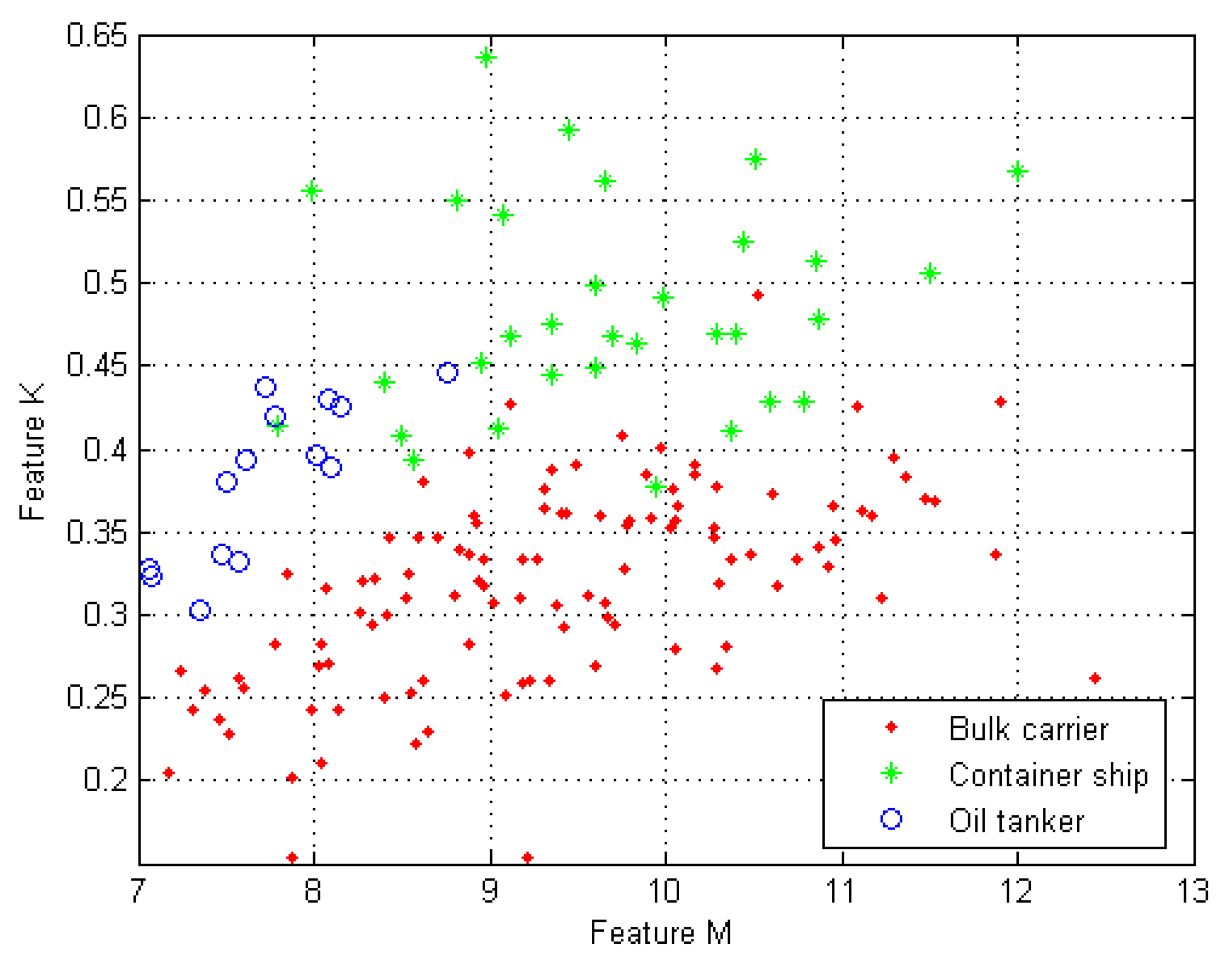
6. Conclusions

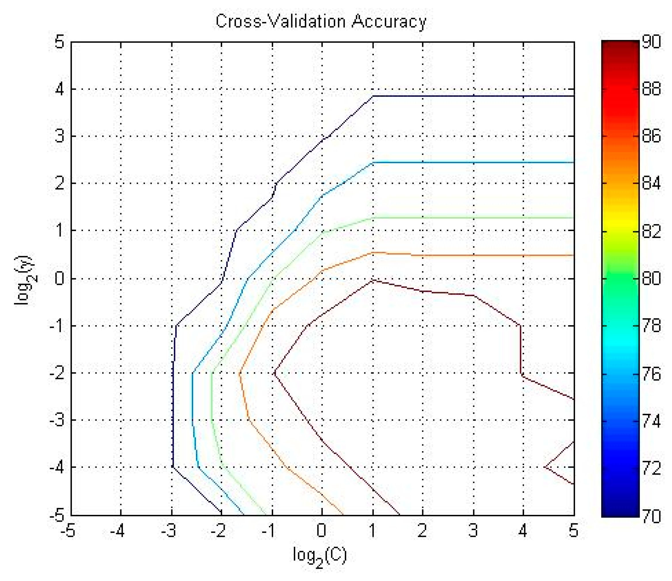
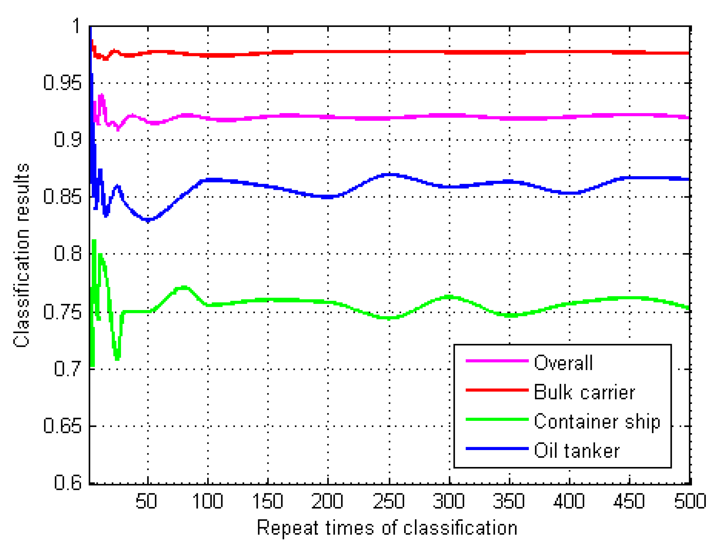
Vessel classification in high-resolution SAR images is highly significant for maritime traffic management and surveillance. In this work, we focus on feature selection and classification of vessels in high-resolution SAR images, present an improved processing procedure and propose feature combinations for vessel classification. In an image, the kernel density estimation can indicate the pixel density and relationship between a pixel and its neighbors. Combined with the mean backscattering coefficient, the feature vector {K, M} (average value of the kernel density estimation and mean backscattering coefficient) has a promising ability to distinguish bulk carriers, container ships and oil tankers. The left-right ratio (R₁), the ratio of the maximum and middle axes (R₂), and the ratio of the maximum and minimum axes (R₃) are three indexes for describing structural features of a vessel. The analysis results show these indexes are better than the local radar cross-section density for vessel classification in high-resolution SAR images. When features R₁, R₂ and R₃ are added to the feature vector {K, M}, the classification results can be slightly improved. The support vector machine is adopted as the classifier. Methods are introduced for the model and parameter selection of the classifier. Before the classification, data normalization is performed with values of every feature to avoid attributes with greater numeric ranges dominating those in smaller numeric ranges. Moreover, the radial basis function is selected as the kernel function for the SVM. The best parameters of the radial basis function are estimated by a “grid search” method for cross validation. The aim of the process is to achieve satisfactory classification results. Lastly, based on feature analysis, the feature vector {K, R₁, R₂, R₃, M} s selected for the classification. The K-nearest neighbor algorithm and minimum distance classifier methods are compared with the proposed method. The results show that the proposed method can obtain better results than the other two methods for classifying the three categories of vessels with 3 m resolution Cosmo-SkyMed stripmap HIMAGE images. The positive classification rates of the algorithm reach 97.6%, 76.3% and 85.9% for the bulk carrier, container ship and oil tanker, respectively. However, because of the “grid search” method for reasonable parameters of the kernel function, the proposed method requires more time than the other two methods.

Although the preliminary results are encouraging, more tests are necessary to improve the classification method. In this paper, only shallow incidence angle, X-band, 3 m resolution SAR images were considered. For steep incidence angles, the method should be adjusted due to the change in the vessel characteristics in the image. As we know, fast ships moving along the azimuth direction are usually strongly blurred and completely out of focused in a SAR image. Even moored ships in high sea states may be blurred due to the radial acceleration generated by sea-wave motion. In these cases, the vessel structures are not clear enough for classification by the method proposed in the paper. Features of travelling ships in the SAR image will be considered in future research. The research area was the open sea. If vessels are anchored in the harbor, a new segmentation method could be developed to isolate the ship signature from quay. To improve the robustness of the method (for example, the threshold in the MER extraction), more images should be obtained for analysis and testing. In addition, the relationship between the physical structures of a vessel and the features in the image under different imaging conditions will be comprehensively investigated.