Article

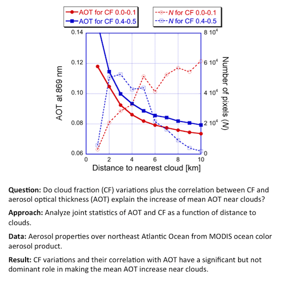
Effect of Cloud Fraction on Near-Cloud Aerosol Behavior in the MODIS Atmospheric Correction Ocean Color Product

by
Tamás Várnai
1,2,* and
Alexander Marshak
2
1
Joint Center for Earth System Technology, University of Maryland Baltimore County, 1000 Hilltop Circle, Baltimore, MD 21250, USA
2
Climate and Radiation Laboratory, NASA Goddard Space Flight Center, 8800 Greenbelt Rd., Greenbelt, MD 20771, USA
*
Author to whom correspondence should be addressed.
Remote Sens. 2015, 7(5), 5283-5299; https://doi.org/10.3390/rs70505283
Submission received: 26 January 2015 / Revised: 16 April 2015 / Accepted: 22 April 2015 / Published: 27 April 2015
(This article belongs to the Special Issue Aerosol and Cloud Remote Sensing)

Abstract

:
Characterizing the way satellite-based aerosol statistics change near clouds is important for better understanding both aerosol-cloud interactions and aerosol direct radiative forcing. This study focuses on the question of whether the observed near-cloud increases in aerosol optical thickness and particle size may be explained by a combination of two factors: (i) Near-cloud data coming from areas with higher cloud fractions than far-from-cloud data and (ii) Cloud fraction being correlated with aerosol optical thickness and particle size. This question is addressed through a statistical analysis of aerosol parameters included in the MODIS (MODerate resolution Imaging Spectroradiometer) ocean color product. Results from ten Septembers (2002–2011) over part of the northeast Atlantic Ocean confirm that the combination of these two factors working together explains a significant but not dominant part (in our case, 15%–30%) of mean optical thickness changes near clouds. Overall, the findings show that cloud fraction plays a large role in shaping the way aerosol statistics change with distance to clouds. This implies that both cloud fraction and distance to clouds are important to consider when aerosol-cloud interactions or aerosol direct radiative effects are examined in satellite or modeling studies.

Graphical Abstract

1. Introduction

During the past decade, a variety of ground-based [1,2,3], aircraft [4,5], and satellite [6,7,8,9] measurements have indicated that aerosol populations are significantly different near clouds and far from clouds. These findings suggest that clouds are surrounded by a several km wide transition zone, where aerosol optical properties and particle size change systematically approaching clouds. Correct interpretation of near-cloud measurements is critical both for assessing aerosol radiative effects—over oceans, about half of all clear-sky columns occur within 4–5 km from low clouds [10,11,12]—and for understanding aerosol-cloud interactions.
The observed near-cloud changes likely come from several reasons, such as aerosols swelling in the humid air surrounding clouds [2,6], or cloud processing that enhances the number of light-scattering aerosol particles through chemical or microphysical processes [13,14]. Moreover, undetected cloud particles—for example in small, evaporating cloud pockets—[15,16], clouds scattering sunlight into nearby clear areas [17,18,19] and even instrument imperfections [10] can also play a role.
Figure 1. Schematic plots illustrating that mean aerosol optical thickness (AOT) can appear to increase towards clouds if the cloud fraction (CF) distribution changes. (a) Hypothetical fractions of samples. Higher and lower CFs are more frequent close to clouds and far from clouds, respectively. (b) Hypothetical mean AOTs. Colored lines correspond to CFs in panel (a). They show AOTs that don’t change near clouds but are correlated with CF. Black line shows overall mean AOT when combining data from all three CFs.
Remotesensing 07 05283 g001
Most recently, analyzing Cloud-Aerosol Lidar and Infrared Pathfinder Satellite Observation (CALIPSO) data, [20] showed (Figure 1) that data sampling can also make overall statistics of aerosol properties change with distance to clouds, given that far-from-cloud aerosol statistics are dominated by data from scenes with lower cloud fraction (CF), while near-cloud aerosol statistics are dominated by data from scenes with higher CF. This may lead to a statistical increase of aerosol optical thickness (AOT) near clouds because, as reported in several papers [21,22,23,24], AOT is positively correlated with CF—though cloud detection uncertainties and 3D radiative processes may make this correlation appear stronger than it really is [19,25,26]. We note that while CF (defined for 30 km and 40 km size areas in [20] and in this paper, respectively) represents large-scale conditions, the distance from the nearest cloud reflects individual pixel conditions.
This paper further explores the contribution of data sampling to the observed near-cloud changes in aerosol statistics. It takes advantage of the unique opportunities of MODerate resolution Imaging Spectroradiometer (MODIS) data products offer for exploring this topic. First, similarly to other imaging radiometers, MODIS can detect clouds that lie outside the satellite track, thus allowing more accurate estimations of both CF and distance to clouds than current spaceborne lidars or radars would allow. (We note that cloud detection has different strengths and limitations when using active instruments or MODIS. For example, while the altitude information helps lidars detect thin cloud layers even when surface properties are not well known, the higher signal-to-noise ratio and wider spectral coverage helps MODIS detect small low-level clouds [27,28].) Second, the MODIS ocean color product provides not only raw radiometric measurements at a resolution sufficiently high for observing systematic trends in near-cloud variations (~1 km) but also aerosol parameters such as optical thickness and Angstrom exponent. Third, some of the quality assessment flags accompanying MODIS data can also help interpret the results.
This outline of this paper is as follows. Section 2 describes our dataset and methodology, Section 3 presents the results, and Section 4 provides a brief summary.

2. Data and Methodology

To help comparisons and putting earlier and current results in context, this paper analyzes a dataset that has been used earlier in [8,29]. (Previously, relationships between aerosol and cloud properties in the study region were also examined in [23].) The data comes from a roughly 1000 km by 500 km region (45°–50°N, 5°–25°W) of the Atlantic Ocean southwest of the United Kingdom (Figure 2). The study uses all daytime MODIS Aqua data from this area for ten two week long periods: 14–29 September in years 2002–2011. The dataset is limited to viewing zenith angles less than 10°.
Figure 2. Map highlighting the study area used in this paper.
Remotesensing 07 05283 g002
The analysis uses aerosol information provided at 1 km resolution in the R2012 version of the MODIS ocean color product [30]: 869 nm aerosol optical thickness, 443 nm–869 nm Angstrom exponent, and various quality assessment (QA) flags. This product is well suited for our study because of its high spatial resolution, its design minimizing uncertainties due to variations in ocean properties, and its extensive set of QA flags.
Similarly to earlier studies [4,6,8,18], we focus on clear areas around low-altitude clouds, as they are most likely to strongly influence nearby aerosols, which are often concentrated at low altitudes. Low clouds are identified using the MODIS cloud mask (MYD35) and cloud product (MYD06), assuming that cloud top pressures over 700 hPa indicate low clouds occurring below ~3 km. For any pixel with aerosol data, the local low CF is calculated by considering a 41 km by 41 km area around the pixel. The low CF is then calculated as the ratio of the number of low cloud pixels to the total number of pixels that are either cloud free or are covered by low clouds. (Pixels with high clouds are excluded, because high clouds can obscure the view and prevent the detection of low clouds below. Moreover, clear-sky pixels are not used if the cloud nearest to them is above 3 km, because high clouds may obscure the view of any low clouds, making it difficult to determine the distance to the nearest low cloud.)

3. Results

This section presents the results in three subsections that discuss observations near low-level clouds by considering (i) all cloud-free areas, (ii) all cloud-free and possibly cloud-contaminated areas, and (iii) cloud-free areas near very thin or small clouds.

3.1. All Cloud-Free Areas

We first examine near-cloud behaviors of aerosol properties by screening our data using all QA flags except for the straylight flag. (We note that all QA flags can take one of two values: “warning” or “no warning”.) The straylight flag is designed to mark areas near bright spots such as thick clouds to ensure that the highly sensitive ocean color retrievals are not biased by instrument stray light contamination [10]. Had we used the straylight flag, we would have been safe even from very small artifacts, but then all information on aerosol properties near thick clouds would have been lost. By not using the straylight flag, we included into our dataset even the areas near thick (bright) clouds.
Figure 3 examines the statistics of our dataset with the goal of confirming our expectations outlined in Figure 1. Panel a confirms the behavior assumed in Figure 1a: As we move farther away from clouds, a higher portion of the data comes from areas with low cloud fractions. Panel b shows that the blue curve is above the red one, which confirms the behavior assumed in Figure 1b: Similarly to the findings of earlier studies [24,31], AOT increases with CF in our dataset as well. On the other hand, Panel b also shows that AOT increases near clouds for any CF. This implies that not all of the near-cloud increases observed in earlier studies can be attributed to the sampling effect outlined in Figure 1 (consisting of the combination of (i) farther from clouds, more of the data comes from areas with low CF, and (ii) lower CF implies lower AOT because of a positive correlation between the two quantities). Panel c shows that the Angstrom exponent (AE) drops near clouds, which indicates larger particle size there. All these behaviors are in qualitative agreement with the findings for CALIPSO data [20].
Additionally, Figure 3c also shows that the AE drop near clouds is especially strong for low CF, perhaps because higher humidity in regions of higher CF keeps particles swollen even in the center of larger clear gaps. Finally, Panel c also shows that AE is larger for larger CF. This is not what one would expect from aerosol humidification or cloud contamination under steady meteorological conditions, and instead may be understood through the following argument. First, there is a positive correlation between AOT and CF (Figure 3b). Second, both our dataset and the MYD04 aerosol product [32] show that in our region, periods of higher AOT come from an increased concentration of small particles that cause higher AEs. We believe that this is neither a microphysical effect nor optical artifact, but an issue of long-range aerosol transport. Most likely, these small particles represent pollution such as sulfate aerosols coming from North America and Europe. The ten separate mean values of AOT and AE for each September in our dataset demonstrate a strong positive correlation (not shown here). We note that in qualitative agreement with these results, MYD04 aerosol data (displayed through NASA’s Giovanni system at http://disc.sci.gsfc.nasa.gov/giovanni) for a full 10-year period shows a positive correlation between monthly mean AOT and AE for our region. As a result, higher CF is associated with higher AOT and, in turn, higher AE.
Figure 4 shows the results as a function of CF at 3 km and 6 km distances from clouds; far enough to reduce the risk of cloud contamination but close enough to see cloud-related effects. Panel a illustrates that, as expected, data from higher CFs is more prevalent closer to clouds. Panels b and c illustrate that, as explained in the previous paragraph, both AOT and AE increase with CF. Panel b also shows that the 869 nm AOT increases with CF at a similar rate near and far from clouds. However, the steeper AE curve at 3 km in Panel c suggests that at shorter wavelengths such as 550 nm, AOT increases faster with CF at 3 km than 6 km. (Given the same 869 nm AOT, larger AE means larger 550 nm AOT. Thus, AE increasing more with CF for D = 3 km means that 550 nm AOT also increases more with CF.)
Figure 3. Impact of distance to cloud for two cloud fraction (CF) ranges. All QA flags are used to screen the data except for the straylight flag. (a) Number of pixels; (b) aerosol optical thickness; (c) Angstrom exponent. In this and subsequent figures, the results for areas less than 2 km away from clouds are shaded because low sample numbers and a higher risk of cloud contamination makes them less reliable. In this and subsequent figures, the error bars indicate the uncertainties due to interannual variability, estimated from the spread of results for individual years. While this figure includes all CF bins below 0.6 (statistics get uncertain for higher CFs), for clarity, subsequent similar figures will include only the 0.0–0.1 and 0.4–0.5 bins (blue and red curves).
Remotesensing 07 05283 g003aRemotesensing 07 05283 g003b
Figure 4. Impact of cloud fraction at two distances from clouds (D = 3 km and D = 6 km). All QA flags are used to screen the data except for the straylight flag. (a) Number of pixels; (b) aerosol optical thickness; (c) Angstrom exponent.
Remotesensing 07 05283 g004aRemotesensing 07 05283 g004b
In order to quantitatively estimate the impact of sampling CFs differently near and far from clouds, [20] resampled their data, such that at any distance from a cloud, the resampled CF distribution matched the CF distribution observed at 10 km. They found that this resampling weakened the near-cloud increase in lidar backscatter and particle size by about 30%. To mitigate the sampling effect highlighted in Figure 1, here we further explore this issue by testing two different resampling methods that exclude some pixels from our calculations of mean AOT and AE. In particular, we reduce the number of used pixels in such ways that at any distance to clouds, CF will be either (method a) uniformly distributed between 0 and 0.6, or (method b) following the original dataset’s overall CF distribution (which combines all available data regardless of distance to cloud).
Figure 5a shows that AOT enhancements are not very sensitive to the sampling of CF, as either method weakens the near-cloud enhancements by about 15%. This insensitivity can be understood by considering that in Figure 3b, the CF-dependence (measured as the difference between blue and red curves) is weaker than the near-cloud increase (measured as the difference between values far and close to a cloud). In contrast, Figure 5b shows that resampling greatly strengthens near-cloud AE changes: For example, the difference between the AEs 2 km and 10 km away from clouds is 3–4 times larger for the resampled data than for the original data. To understand why resampling and its exact method make a big difference for AE, we need to consider that in Figure 3c, CF-dependence is comparable or even stronger than the near-cloud change (i.e., the distance between the red and blue curves is comparable to the near-cloud change for either of these curves). The strong CF dependence implies that the results might be different if we use different resampling schemes for combining the various CF curves into a single overall curve.
The finding in Figure 5b that resampling to a constant CF strengthens near-cloud AE-changes is opposite to the findings in [20]. The strengthening comes from the positive correlation (discussed at Fig 3c) between CF and AE in our multi-September dataset: When we resample our data to a constant CF distribution, we increase the weight of low CFs (hence low AEs) near clouds, while far from clouds, we increase the weight of high CFs (hence high AEs).
Figure 5. Near-cloud changes in (a) AOT and (b) AE, when data from all CFs is combined in various ways. Blue (original): all data; Red (method a): At all distance bins, the CF distribution is resampled to a uniform distribution ranging from 0 to 0.6; Green (method b): At all distance bins, the CF distribution is resampled to the overall CF distribution. All QA flags are used to screen the data except for the straylight flag.
Remotesensing 07 05283 g005

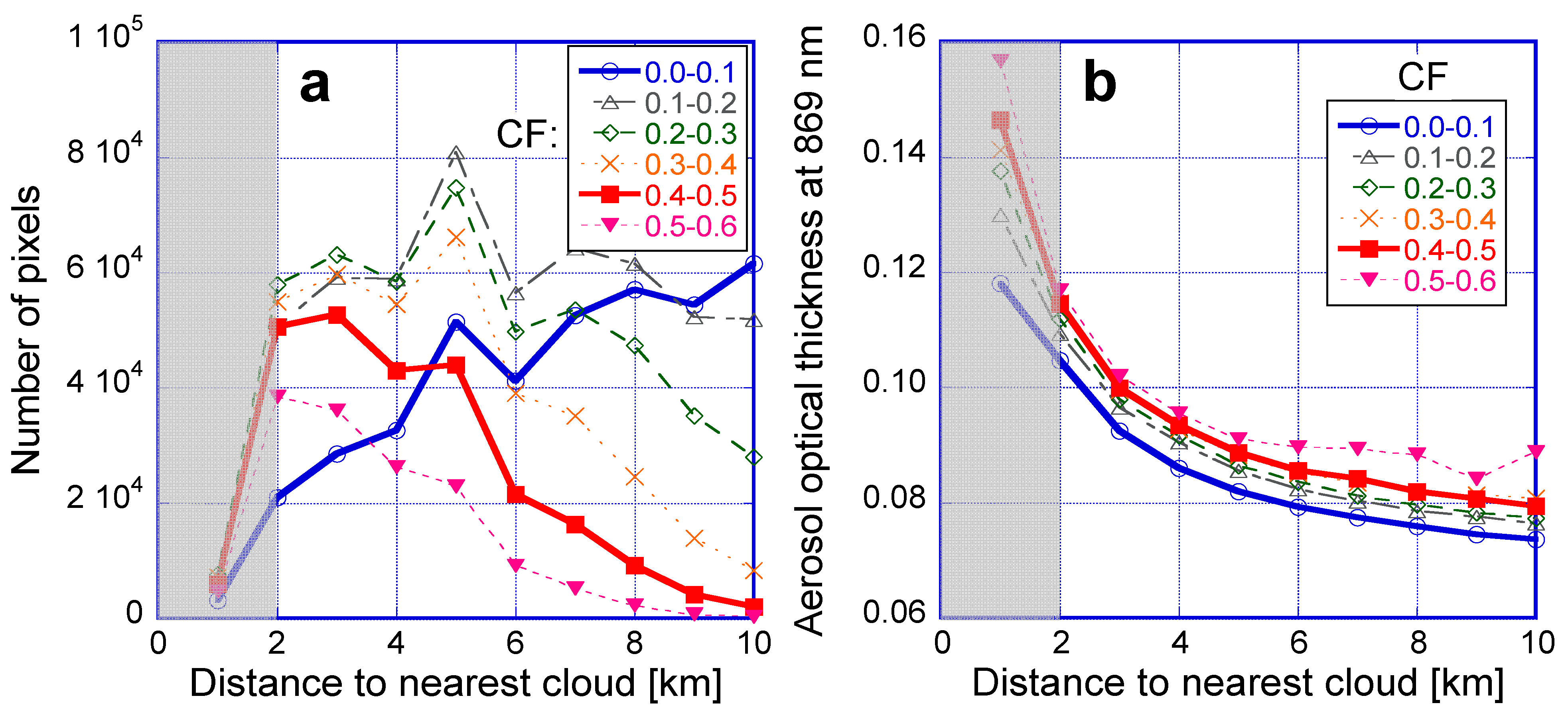
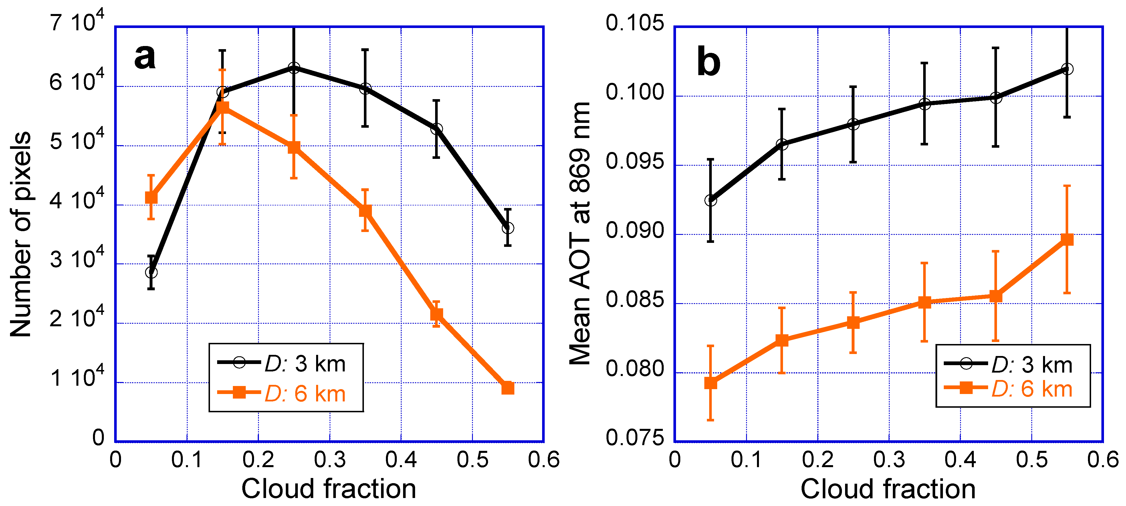
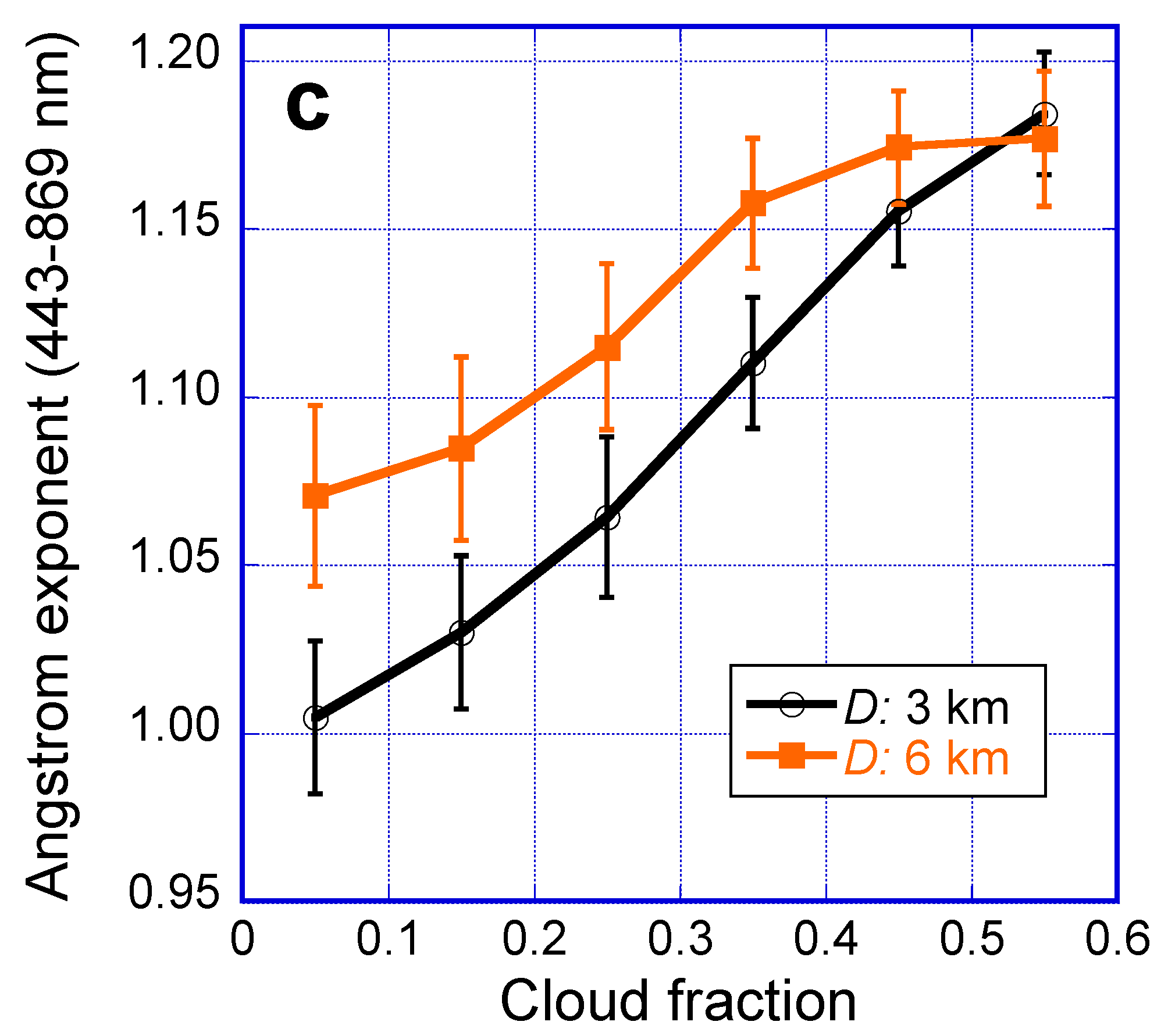
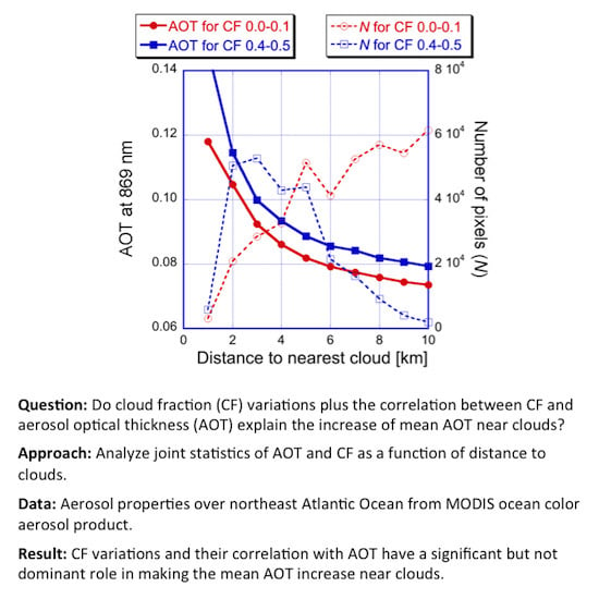
3.2. All Cloud-Free and Possibly Cloud-Contaminated Areas

In this section we examine the way Figure 3, Figure 4 and Figure 5 change if, in addition to ignoring the straylight flag, our data selection also ignores warnings by the sstwarn QA flag described in Table 1. Ignoring the sstwarn flag allows one to consider even the pixels where the aerosol population is somewhat similar to cloud droplets due to a significant number of large particles (such as desert dust grains). On the other hand, ignoring the sstwarn also raises the possibility of cloud contamination (the presence of cloud droplets in atmospheric columns deemed cloud free by the cloud mask), mostly by thin cirrus or very small cumulus clouds [33].
Figure 6 shows that ignoring the sstwarn flag doesn’t change the basic tendencies we saw in Figure 3. If anything, the tendencies of Figure 3 get amplified: The sampling of CF becomes more uneven and, for higher cloud fraction, the AE decrease near clouds gets stronger. As expected, the impact is strongest for higher CFs, as having more clouds intensifies cloud and cloud-related meteorological effects on nearby clear areas, and makes the presence of undetected cloud pieces more likely. The impact of ignoring the sstwarn flag extends far from clouds because cloud contamination by thin cirrus can occur even far from any detected low clouds.
Table 1. List of the tests considered by the operational MODerate resolution Imaging Spectroradiometer (MODIS) ocean color data processing for setting the sstwarn flag. The flag is set if the total number of warning points is 1, 2, or 3. (Pixels with more warning points are flagged by the sstfail flag and are not used.) A detailed description of sstwarn flag is at http://oceancolor.gsfc.nasa.gov/DOCS/modis_sst/.
TestPoints Added If Failing Test
Brightness temperature is outside the −4 °C to 33 °C range3
Retrieved SST is outside the −2 °C to 45 °C range3
Difference between retrieved and expected SST exceeds 3 °C or 6 °C1 or 3
Difference between min. and max. SST values in 3 × 3 km surroundings exceeds 0.7 °C or 1.2 °C2 or 3
Difference between min. and max. 678 nm reflectance in 3 × 3 km surroundings exceeds 0.012
Sensor zenith angle exceeds 55° or 75°1 or 3
Figure 7b shows that not using the sstwarn flag increases the AOT vs. CF slope by about 50%. This indicates that CF has especially strong effects on pixels flagged by sstwarn. For example, pixels deemed cloud free by the cloud mask may be especially sensitive to CF-related conditions (e.g., humidity, prevalence of updrafts) if they contain detrained cloud droplets or large aerosols that can grow substantially in modest updrafts—and hence are flagged by sstwarn.
In contrast, Figure 7c shows that not using the sstwarn flag decreases the AE vs. CF slope by about a third, giving the impression that particle size in pixels flagged by sstwarn is not really sensitive to CF. This impression, however, is somewhat misleading: The undetected droplets or large aerosols that trigger the sstwarn flag create a strong CF-sensitivity for both AOT and particle size. For particle size, however, this strong effect acts to weaken the even stronger opposite effect discussed at Figure 3c: High AOT and CF in this region is often associated with high concentrations of small pollution particles, which causes AE to increase with CF—albeit the increase is weaker for the sstwarn-flagged pixels, which are especially susceptible to local humidity and cloud effects.
Figure 8a shows that when not using the sstwarn flag, resampling our dataset to a constant CF distribution weakens the near-cloud AOT increase by 30% for either resampling method (in contrast to the 15% weakening when the sstwarn flag was used in Figure 5). Figure 8b shows that when not using the sstwarn flag, resampling by any method increases the near-cloud AE drop of the original dataset (which combines all data for any CF) by more than a third.

3.3. Cloud-Free Areas Near Very Thin or Small Clouds

Finally, let us examine how the results change if we use all QA flags for data screening. Using even the straylight flag implies that we exclude areas near bright clouds, and keep only the areas near clouds that are too thin or small to trigger a straylight warning. Figure 9 shows that the results are very similar to Figure 3 farther than 5 km away from clouds, where the straylight flag is hardly ever set. Near clouds, however, the sample numbers drop drastically in Panel a, as only the clear pixels near very thin clouds remain. Panel b shows that the thin clouds (or small cloud puffs) that don’t trigger a straylight warning have only a weak effect on AOT. Panel c—and its comparison to Figure 6c—reveals that using a more restrictive data selection yields higher AE, that is, smaller particle size. For low CF, particle size still increases towards clouds, but the increase is weaker than it was for the more inclusive data selections in Figure 6c. (The changes appear strong right near clouds, but this likely comes from the low sample numbers and/or cloud contamination.) For higher CF, AE remains steady past 2 km from clouds, perhaps because particle populations may be dominated by small pollution particles that might be below or above cloud altitude, or because the higher humidity keeps particles swollen even in the center of clear gaps.
Figure 6. Same as Figure 3 (solid lines), but also showing the results (dashed lines) when the data selection ignores warnings by both the straylight (marked strl) and sstwarn (marked sstw) QA flags. (a) Number of pixels; (b) Aerosol optical thickness; (c) Angstrom exponent.
Remotesensing 07 05283 g006
Figure 7. Same as Figure 4 (solid lines), but also showing the results (dashed lines) when the data selection ignores warnings by both the straylight and sstwarn QA flags. (a) Number of pixels; (b) Aerosol optical thickness; (c) Angstrom exponent.
Remotesensing 07 05283 g007
The final figure, Figure 10, shows that AOT and AE both increase with CF, though the AOT increase is weaker than in Figure 4. The AE increase is especially significant and, as discussed earlier, may be due to small pollution particles in cloudier periods.
Figure 8. Same as Figure 5, but with the data selection ignoring warnings by both the straylight and sstwarn QA flags. (a) Aerosol optical thickness; (b) Angstrom exponent.
Remotesensing 07 05283 g008
Figure 9. Same as Figure 3, but with the data selection using warnings by all QA flags. (a) Number of pixels; (b) Aerosol optical thickness; (c) Angstrom exponent.
Remotesensing 07 05283 g009
Figure 10. Same as Figure 4, but with the data selection using warnings by all QA flags. (a) Number of pixels; (b) Aerosol optical thickness; (c) Angstrom exponent.
Remotesensing 07 05283 g010

4. Conclusions

This study used satellite data to examine the way aerosol particles change in the vicinity of clouds. In particular, it investigated whether the near-cloud increases in optical thickness and particle size found in earlier studies may be explained by the combination of two factors: (i) Near-cloud data coming from areas with higher cloud fractions than far-from-cloud data and (ii) Cloud fraction being correlated with aerosol optical thickness and particle size. In addressing this issue, the paper presented a statistical analysis of aerosol optical thickness and Angstrom exponent values reported in the MODIS ocean color product as a function of cloud fraction and distance to cloud. Using MODIS data allowed this study to examine retrieved aerosol properties as opposed to raw radiometric data, and also to consider off-track clouds in characterizing local cloud fraction and distance to clouds. The analysis used data collected over the northeast Atlantic Ocean during ten consecutive Septembers.
Similar to the analysis of CALIPSO data [20], the results of MODIS data analysis showed that sampling of different cloud fractions near clouds and far from clouds can explain a significant but not dominant part (15%–30%) of the near-cloud AOT changes reported earlier [29]. For particle size, however, analyzing the Atlantic Ocean southwest of the United Kingdom yielded some opposite behaviors than the area near the Azores [20]: While sampling different cloud fractions near and far from clouds strengthened the near-cloud particle size changes in the composite statistics of the Azores, this effect weakened the near-cloud particle size changes in our composite statistics. The opposite behavior arises because in our dataset, particle size decreases with the increase of cloud fraction, as cloudier air coming from North America or Europe contains smaller pollution particles than the more clear air containing larger sea salt or desert dust particles. The differences between results for our study region and the region around the Azores confirm the earlier finding that near-cloud behaviors display significant variability across the globe [34].
Accordingly, we found that resampling our data to a constant cloud fraction distribution (that doesn’t change with distance to clouds) makes observed near-cloud optical thickness changes slightly weaker. In contrast, the resampling made near-cloud particle size changes even stronger in our dataset—which implies that resampling would strengthen the particle size changes discussed in [29]. We also found that the exact method of resampling makes very little difference for optical thickness, and only a modest difference for particle size (characterized through the Angstrom exponent).
Finally, the results revealed that the way aerosol statistics change with distance to clouds or cloud fraction depends on which MODIS-provided quality assessment (QA) flags we use for data screening. When all QA flags are used, near-cloud data is kept only if the nearby clouds are very thin—and so aerosol changes with distance to cloud or cloud fraction are very weak. When warnings by the straylight QA flag are ignored, the dataset will include areas near thick clouds as well, resulting in aerosol statistics that change markedly with both distance to cloud and cloud fraction. When warnings by the sstwarn flag are also ignored, data with somewhat cloud-like aerosol populations are also included even at the risk of some cloud contamination—and this results in even stronger changes in aerosol statistics with both distance to cloud and cloud fraction.
Overall, the findings highlight that cloud fraction plays a significant role in shaping the way aerosol statistics change with distance to clouds. This implies that both cloud fraction and distance to clouds are important to consider in satellite studies and modeling of aerosol-cloud interactions or aerosol direct radiative effects.

Acknowledgments

We gratefully acknowledge support for this research by the NASA Radiation Sciences Program managed by Hal Maring and by the NASA CALIPSO project supervised by Charles Trepte as the technical officer. We also thank Ziauddin Ahmad, Bryan Franz, Gerhard Meister, and other members of the MODIS ocean color team, as well as Bob Charlson, Larry Di Girolamo, Robert Levy, Alexei Lyapustin, Guoyong Wen, Rob Wood, and Weidong Yang for insightful discussions and help. We are also grateful to the three anonymous reviewers, who helped greatly to improve the manuscript.

Author Contributions

Authors Várnai and Marshak collaborated closely and used frequent discussions to design the experiments and to interpret and present the results. Tamás Várnai performed the actual calculations.

Conflicts of Interest

The authors declare no conflict of interest.

References

  1. Koren, I.; Remer, L.A.; Kaufman, Y.J.; Rudich, Y.; Martins, J.V. On the twilight zone between clouds and aerosols. Geophys. Res. Lett. 2007, 34, L08805. [Google Scholar]
  2. Jeong, M.J.; Li, Z. Separating real and apparent effects of cloud, humidity, and dynamics on aerosol optical thickness near cloud edges. J. Geophys. Res. 2010, 115, D00K32. [Google Scholar]
  3. Eck, T.F.; Holben, B.N.; Reid, J.S.; Arola, A.; Ferrare, R.A.; Hostetler, C.A.; Crumeyrolle, S.N.; Berkoff, T.A.; Welton, E.J.; Lolli, S.; et al. Observations of rapid aerosol optical depth enhancements in the vicinity of polluted cumulus clouds. Atmos. Chem. Phys. 2014, 14, 11633–11656. [Google Scholar] [CrossRef] [Green Version]
  4. Su, W.; Schuster, G.L.; Loeb, N.G.; Rogers, R.R.; Ferrare, R.A.; Hostetler, C.A.; Hair, J.W.; Obland, M.D. Aerosol and cloud interaction observed from high spectral resolution lidar data. J. Geophys. Res. 2008, 113, D24202. [Google Scholar] [CrossRef]
  5. Redemann, J.; Zhang, Q.; Russell, P.B.; Livingston, J.M.; Remer, L.A. Case studies of aerosol remote sensing in the vicinity of clouds. J. Geophys. Res. 2009, 114, D06209. [Google Scholar]
  6. Twohy, C.H.; Coakley, J.A., Jr.; Tahnk, W.R. Effect of changes in relative humidity on aerosol scattering near clouds. J. Geophys. Res. 2009, 114, D05205. [Google Scholar]
  7. Tackett, J.L.; Di Girolamo, L. Enhanced aerosol backscatter adjacent to tropical trade wind clouds revealed by satellite-based lidar. Geophys. Res. Lett. 2009, 36, L14804. [Google Scholar] [CrossRef]
  8. Várnai, T.; Marshak, A. MODIS observations of enhanced clear sky reflectance near clouds. Geophys. Res. Lett. 2009, 36, L06807. [Google Scholar] [CrossRef]
  9. Yang, W.; Marshak, A.; Kostinski, A.B.; Várnai, T. Shape-induced gravitational sorting of Saharan dust during transatlantic voyage: Evidence from CALIOP lidar depolarization measurements. Geophys. Res. Lett. 2013, 40, 3281–3286. [Google Scholar] [CrossRef]
  10. Meister, G.; McClain, C.R. Point-spread function of the ocean color bands of the Moderate Resolution Imaging Spectroradiometer on Aqua. Appl. Opt. 2010, 49, 6276–6285. [Google Scholar] [CrossRef] [PubMed]
  11. Várnai, T.; Marshak, A. Global CALIPSO observations of aerosol changes near clouds. Geosci. Remote Sens. Lett. 2011, 8, 19–23. [Google Scholar] [CrossRef]
  12. Várnai, T.; Marshak, A. Analysis of co-located MODIS and CALIPSO observations near clouds. Atmos. Meas. Tech. 2012, 5, 389–396. [Google Scholar] [CrossRef]
  13. Kerkweg, A.; Wurzler, S.; Reisin, T.; Bott, A. On the cloud processing of aerosol particles: An entraining air-parcel model with two-dimensional spectral cloud microphysics and a new formulation of the collection kernel. Q. J. Roy. Meteorol. Soc. 2003, 129, 1–18. [Google Scholar] [CrossRef]
  14. Ervens, B.; Turpin, B.J.; Weber, R.J. Secondary organic aerosol formation in cloud droplets and aqueous particles (aqSOA): A review of laboratory, field and model studies. Atmos. Chem. Phys. 2011, 11, 11069–11102. [Google Scholar] [CrossRef]
  15. Charlson, R.; Ackerman, A.; Bender, F.; Anderson, T.; Liu, Z. On the climate forcing consequences of the albedo continuum between cloudy and clear air. Tellus 2007, 59, 715–727. [Google Scholar] [CrossRef]
  16. Koren, I.; Feingold, G.; Jiang, H.; Altaratz, O. Aerosol effects on the inter-cloud region of a small cumulus cloud field. Geophys. Res. Lett. 2009, 36, L14805. [Google Scholar] [CrossRef]
  17. Kassianov, E.I.; Ovtchinnikov, M. On reflectance ratios and aerosol optical depth retrieval in the presence of cumulus clouds. Geophys. Res. Lett. 2008, 35, L06807. [Google Scholar] [CrossRef]
  18. Wen, G.; Marshak, A.; Cahalan, R.F.; Remer, L.A.; Kleidman, R.G. 3-D aerosol-cloud radiative interaction observed in collocated MODIS and ASTER images of cumulus cloud fields. J. Geophys. Res. 2007, 112, D13204. [Google Scholar]
  19. Marshak, A.; Wen, G.; Coakley, J.; Remer, L.A.; Loeb, N.G.; Cahalan, R.F. A simple model for the cloud adjacency effect and the apparent bluing of aerosols near clouds. J. Geophys. Res. 2008, 113, D14S17. [Google Scholar]
  20. Yang, W.; Marshak, A.; Várnai, T.; Wood, R. CALIPSO observations of near-cloud aerosol properties as a function of cloud fraction. Geophys. Res. Lett. 2014, 41, 9150–9157. [Google Scholar] [CrossRef]
  21. Loeb, N.G.; Manalo-Smith, N. Top-of-atmosphere direct radiative effect of aerosols over global oceans from merged CERES and MODIS observations. J. Climate 2005, 18, 3506–3526. [Google Scholar] [CrossRef]
  22. Kaufman, Y.J.; Koren, I.; Remer, L.A.; Tanré, D.; Ginoux, P.; Fan, S. Dust transport and deposition observed from the Terra-Moderate Resolution Imaging Spectroradiometer (MODIS) spacecraft over the Atlantic Ocean. J. Geophys. Res. 2005, 110, D10S12. [Google Scholar] [CrossRef]
  23. Matheson, M.A.; Coakley, J.A., Jr.; Tahnk, W.R. Aerosol and cloud property relationships for summertime stratiform clouds in the northeastern Atlantic from AVHRR observations. J. Geophys. Res. 2005, 110, D24204. [Google Scholar] [CrossRef]
  24. Chand, D.; Wood, R.; Ghan, S.J.; Wang, M.; Ovchinnikov, M.; Rasch, P.J.; Miller, S.; Schichtel, B.; Moore, T. Aerosol optical depth increase in partly cloudy conditions. J. Geophys. Res. 2012, 117, D17207. [Google Scholar]
  25. Ignatov, A.; Minnis, P.; Loeb, N.G.; Wielicki, B.; Miller, W.; Sun-Mack, S.; Tanre, D.; Remer, L.A.; Laszlo, I.; Geier, E. Two MODIS aerosol products over ocean on the Terra and Aqua CERES SSF. J. Atmos. Sci. 2005, 62, 1008–1031. [Google Scholar] [CrossRef]
  26. Zhang, J.; Christopher, S.A.; Remer, L.A.; Kaufman, Y.J. Shortwave aerosol radiative forcing over cloud-free oceans from Terra: 1. Angular models for aerosols. J. Geophys. Res. 2005, 32, D10S23. [Google Scholar]
  27. Holz, R.E.; Ackerman, S.A.; Nagle, F.W.; Frey, R.; Dutcher, S.; Kuehn, R.E.; Vaughan, M.A.; Baum, B. Global moderate resolution imaging spectroradiometer (MODIS) cloud detection and height evaluation using CALIOP. J. Geophys. Res. 2008, 113, D00A19. [Google Scholar]
  28. Chan, M.A.; Comiso, J.C. Cloud features detected by MODIS but not by CloudSat and CALIOP. Geophys. Res. Lett. 2011, 38, L24813. [Google Scholar] [CrossRef]
  29. Várnai, T.; Marshak, A. Near-cloud aerosol properties from the 1 km resolution MODIS ocean product. J. Geophys. Res. 2014, 119, 1546–1554. [Google Scholar] [CrossRef]
  30. Ahmad, Z.; Franz, B.A.; McClain, C.R.; Kwiatkowska, E.J.; Werdell, J.; Shettle, E.P.; Holben, B.N. New aerosol models for the retrieval of aerosol optical thickness and normalized water-leaving radiances from the SeaWiFS and MODIS sensors over coastal regions and open oceans. Appl. Opt. 2010, 49, 5545–5560. [Google Scholar] [CrossRef] [PubMed]
  31. Loeb, N.G.; Schuster, G.L. An observational study of the relationship between cloud, aerosol and meteorology in broken low-level cloud conditions. J. Geophys. Res. 2008, 113, D14214. [Google Scholar] [CrossRef]
  32. Remer, L.A.; Kaufman, Y.J.; Tanre, D.; Mattoo, S.; Chu, D.A.; Martins, J.V.; Li, R.R.; Ichoku, C.; Levy, R.C.; Kleidman, R.G.; et al. The MODIS aerosol algorithm, products and validation. J. Atmos. Sci. 2005, 62, 947–973. [Google Scholar] [CrossRef]
  33. Koren, I.; Oreopoulos, L.; Feingold, G.; Remer, L.A.; Altaratz, O. How small is a small cloud? Atmos. Chem. Phys. 2008, 8, 6379–6407. [Google Scholar] [CrossRef]
  34. Várnai, T.; Marshak, A.; Yang, W. Multi-satellite aerosol observations in the vicinity of clouds. Atmos. Chem. Phys. 2013, 13, 3899–3908. [Google Scholar] [CrossRef]

