Article

A Quantitative Inspection on Spatio-Temporal Variation of Remote Sensing-Based Estimates of Land Surface Evapotranspiration in South Asia

Institute of Mountain Hazards and Environment, Chinese Academy of Sciences, Chengdu 610041, China
*
Author to whom correspondence should be addressed.
These authors contributed equally to this work.
Remote Sens. 2015, 7(4), 4726-4752; https://doi.org/10.3390/rs70404726
Submission received: 21 January 2015 / Revised: 25 March 2015 / Accepted: 13 April 2015 / Published: 17 April 2015
(This article belongs to the Special Issue Recent Advances in Thermal Infrared Remote Sensing)

Abstract

:
Evapotranspiration (ET) plays a key role in water resource management. It is important to understand the ET spatio-temporal pattern of South Asia for understanding and anticipating serious water resource shortages. In this study, daily ET in 2008 was estimated over South Asia by using MODerate Resolution Imaging Spectroradiometer (MODIS) products combined with field observations and Global Land Data Assimilation System (GLDAS) product through Surface Energy Balance System (SEBS) model. Monthly ET data were calculated based on daily ET and evaluated by the GLDAS ET data. Good agreements were found between two datasets for winter months (October to February) with R2 from 0.5 to 0.7. Spatio-temporal analysis of ET was conducted. Ten specific sites with different land cover types at typical climate regions were selected to analyze the ET temporal change pattern, and the result indicated that the semi-arid or arid areas in the northwest had the lowest average daily ET (around 0.3 mm) with a big fluctuation in the monsoon season, while the sites in the Indo-Gangetic Plain and in southern India has bigger daily ET (more than 3 mm) due to a large water supplement. It is suggested that the monsoon climate has a large impact on ET spatio-temporal variation in the whole region.

Graphical Abstract

1. Introduction

Evapotranspiration (ET) is the sum of evaporation from the soil surface and plant transpiration to the atmosphere. It is an essential part of water balance with a central role also in energy and carbon balance, and plays a key part in the hydrological process. Because it is the biggest cause of loss of land water, the assessment of ET is of outstanding importance for water resource management, planning, and monitoring [1,2].
South Asia is home to one-fourth of the global population, with access only to less than 5 percent of the planet’s freshwater resources. The depletion of water resources due to climate change or the mismanagement of water resources by the countries concerned has become a looming crisis and a threat to the lives and the livelihoods of the people of South Asia [3]. Meanwhile, the precipitation is unevenly distributed throughout South Asia with the rainfall events varying significantly from year to year and month to month. A recent study of the monsoon season over the last sixty years reveals that the intensity of extreme precipitation and the number of very dry spells have both been increasing [4]. The extremes of rainfall and dry season cause severe drought and flood disasters which gravely threaten the agricultural production, economic development and social security of the countries in South Asia [5,6]. As a vital component in water balance, a quantitative and accurate depiction of ET distribution in South Asia becomes more and more urgent for the water resources management and planning required to face the impending problems and disasters. However, since South Asia is mainly composed of less-developed countries, few field surface energy flux observation sites are established over this region. Former studies [7,8] were usually conducted using estimations based on meteorological stations using the Penman-Monteith method, which also makes it difficult to attain the spatial information.
Fortunately, the rapid development of remote sensing techniques in recent years opens a new era of retrieval and monitoring of land surface parameters (such as land surface temperature, energy fluxes, vegetation variables, and soil moisture)—from the local to global scales—with different temporal frequency and spatial resolution. It also provides a vital way to get land surface ET spatial and temporal distribution in South Asia. Recently, a few approaches to remote sensing based on ET estimation methods have been proposed and widely applied around the world [9,10,11,12,13,14,15]. Among these methods, the physical methods based on surface energy balance form a big group from which one can derive ET, including the commonly used Surface Energy Balance Algorithm over Land (SEBAL) [16], Simplified Surface Energy Balance Index (S-SEBI) [17], Surface Energy Balance System (SEBS) [18], and Mapping Evapotranspiration with Internalized Calibration (METRIC) [19]. As a common approach, the SEBS model has been widely validated by many researchers at different locations with different climatic and land cover conditions [12,20,21,22,23]. Compared with other surface energy balance based methods, Timmermans, et al. [22] has pointed out the special advantages of SEBS: (i) a more physically based parameterization of the turbulent heat fluxes for different states of the land surface and the atmosphere; (ii) a feasible minimum number of required input variables. These advantages enable the SEBS model to be chosen as the baseline algorithm within the Water Cycle Multi-Mission Observation Strategy (WACMOS) to produce global fluxes. Meanwhile, it has been also evaluated around the world and applied to map ET from field [24], regional [25] and global [26] scales. Therefore, the SEBS model was selected as the basic method to map the ET distribution in South Asia in this study.
In the SEBS model, atmospheric parameters such as near surface air temperature, humidity, and air pressure are important auxiliary inputs; the uncertainty in atmospheric inputs will greatly affect the estimation of surface energy fluxes and ET [27]. In South Asia, the available meteorological stations are sparsely distributed over the subcontinent, which induces large uncertainties to get the regional distribution of atmospheric parameters according to the limited stations. To overcome this problem, we proposed a practical method by combining the in situ meteorological observations with the Global Land Data Assimilation System (GLDAS) 3-hourly product to downscale the atmospheric data during the satellite overpass time at the satellite data spatial resolution, and then retrieve surface energy fluxes by the SEBS model with MODerate Resolution Imaging Spectroradiometer (MODIS) products with the downscaled atmospheric data in South Asia [28]. By applying the above method, we derive the time series of ET maps of South Asia in 2008.

2. Study Area and Data Sources
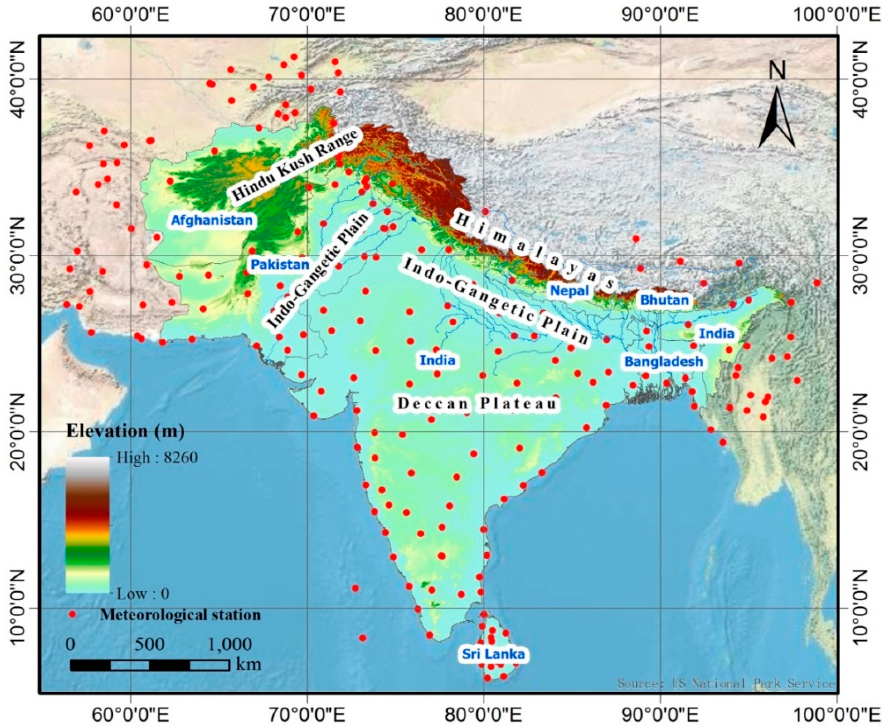
2.1. Study Area

The core countries of South Asia are selected as the study area which includes India, Pakistan, Afghanistan, Nepal, Bhutan, Sri Lanka and Bangladesh (Figure 1).
Figure 1. Core countries and the locations of available meteorological stations around South Asia.
Remotesensing 07 04726 g001
This vast region is home to a variety of geographical features, such as glaciers, rainforests, valleys, deserts, and grasslands. The typical terrain feature is the Hindu Kush Range and the Himalayas in the north, the Indo-Gangetic Plain in the Indus River and the Ganges River basin, the Thar Desert located in the northwestern India and eastern Pakistan, and the Deccan Plateau in the middle and south. Its climate varies considerably, with the dry subtropical continental climate in the northern Indian edge and northern Pakistani uplands, the equatorial climate in the far south of India and southwest Sri Lanka, the hot subtropical climate in northwest India, the cool winter, hot tropical climate in Bangladesh, the tropical semi-arid climate in the center and the Alpine climate in the Himalayas. The climate differences are influenced by not only the latitude and altitude, but also by factors such as proximity to the sea coast and the seasonal impact of the monsoons. The winter monsoon is usually from September to March, while the summer monsoon is usually from June to September and accounts for 70%–90% of the annual precipitation. This nonuniform distribution of rainfall induces the water resources to have significant spatial and temporal variability.

2.2. Data Sources

In the time series ET estimation, the input data generally include three types: satellite data from TERRA-MODIS products provided by NASA’s Earth Observation System Data and Information System (https://earthdata.nasa.gov/), hourly and daily atmospheric data from meteorological stations’ observations provided by the Climate Data Online (CDO) of National Climatic Data Center (NCDC) (http://www.ncdc.noaa.gov/cdo-web/), and the assimilation products provided by the Global Land Data Assimilation System (GLDAS) (http://disc.sci.gsfc.nasa.gov/hydrology/data-holdings).
For satellite data, the products include 1 km MODIS daily land surface temperature/emissivity (MOD11_L2), 1 km 16-Day vegetation indices (MOD13A2), Calibrated Radiances (MOD021KM), Geolocation (MOD03), 1 km Atmospheric Precipitable Water (MOD05_L2), 1 km Leaf Area Index (LAI) (MOD15A2), 1 km 16-Day albedo (MCD43B3), and 500 m Land Cover Type (MCD12Q1). The spatial resolution of the land cover product is rescaled to 1 km to make sure all these products have the same spatial resolution.
The atmospheric observation data include near surface air temperature, relative humidity, air pressure, wind speed and direction, dew point temperature, and ceiling height. The observation frequency at different stations changes from hourly to several hours. To get reliable spatial distributed atmospheric data, 233 stations not only in South Asia but also from neighboring countries such as Iran, Tajikistan, Turkmenistan, Uzbekistan, Burma and China are involved in this study. The spatial location of the meteorological stations is pointed out in Figure 1.
GLDAS drives multiple, offline (not coupled to the atmosphere) land surface models: Mosaic, Noah, the Community Land Model (CLM), and the Variable Infiltration Capacity (VIC), integrate a huge quantity of observation-based data, and executes globally at resolutions from 2.5 degrees to 1 km, enabled by the Land Information System (LIS) [29,30]. In this current study, we choose the 3-hourly and monthly high resolution (0.25 degrees) assimilation data run by the Noah model. The atmospheric forcing data such as specific humidity at 2 m (kg·kg−1), wind speed at 10 m (m·s−1), air temperature at 2 m (K), and air pressure (Pa), can be provided in the 3-hourly file. This file is helpful for the ET estimation. Monthly average ET in the monthly file is used to cross-validate the ET estimation results.

3. Method

3.1. Surface Energy Balance System (SEBS) Model

The SEBS model is a single source model based on surface energy balance which was proposed to estimate atmospheric turbulent fluxes, the evaporative fraction, and actual ET using remote sensing data combined with land surface meteorological observation information [18]. It consists of: (1) an estimation of a series of land surface physical parameters, such as emissivity, albedo, vegetation coverage etc. based on spectral reflectance and radiance; (2) an extended model of roughness length estimation for heat transfer; (3) an evaporative fraction estimation for limiting cases by energy balance.
The energy balance computation at limiting conditions (dry limit and wet limit) is used in order to derive the relative evaporation. At the wet limit, the latent heat flux is only constrained by the available energy and the atmospheric conditions, and the sensible heat flux reaches the minimum value, described as:
H w e t = R n G 0 L E w e t
At the dry limit, the latent heat flux is close to zero, and the sensible heat flux is at the maximum value:
H d r y = R n G 0
Finally, the sensible heat flux estimation in this model is constrained to the range set from the wet limit (Hwet) to the dry limit (Hdry). Then, the relative evaporation (Λr) is expressed as:
Λ r = 1 H H w e t H d r y H w e t
With the knowledge of Rn; G and latent heat flux at wet limit (LEwet); the evaporative fraction (Λ) is finally determined as:
Λ = L E R n G = Λ r L E w e t R n G
The major inputs include: (1) remote sensing data: albedo, land surface emissivity, land surface temperature (LST), leaf area index (LAI) and the Normalized Difference Vegetation Index (NDVI); (2) Meteorological data (near surface air pressure, air temperature, relative humidity and wind speed); and (3) Radiation data (surface net shortwave radiation and surface net longwave radiation). The parameterizations of surface net shortwave radiation and surface net longwave radiation were based on the methods proposed by Tang, et al. [31] and Tang and Li [32]. For soil heat flux, it was calculated as a ratio of surface net radiation according to the expression below:
G = R n ( Γ c + ( 1- f c ) ( Γ s - Γ c ) )
where Γc = 0.05 for full vegetation canopy and Γs = 0.315 for bare soil. fc is the vegetation fraction cover determined by the formula proposed by Carlson and Ripley [33] :
f c = ( N D V I N D V I min N D V I max N D V I min ) 2
where NDVImin and NDVImax are the NDVI values of bare soil and fully vegetated surface. They are simply assigned to 0.2 and 0.86, respectively [14,23,34]. The pixel with NDVI below 0.2 is thought to be bare soil, and above 0.86 is thought to be a fully vegetated surface.
According to the SEBS method, the auxiliary data, especially the atmospheric data, play an important role in the final estimation results. To maintain the high accuracy of atmospheric data and avoid the uncertainty of directly downscaling air temperature from GLDAS product to satellite resolution, Zhao, et al. [28] proposed a linear fit method between the observed air temperature from meteorological stations and the downscaled air temperature from GLDAS products to calibrate the accuracy of the downscaled air temperature. The estimation results showed a big improvement against the simple use of the downscaled air temperature or interpolated air temperature from field observation.
However, the stations distributed over the vast region demonstrate that large differences in latitude and altitude directly or indirectly affect air temperature. The latitude controls the solar irradiance to influence the surface heating process and the air temperature change. For altitude, a negative correlation exists between altitude and near surface air temperature with the lapse rate of about 0.6 °C per 100 m. Therefore, a small modification was made to the method by importing both latitude and altitude into the calibration work by using multiple variable linear fit method to consider the impacts from them on air temperature variation. The expression is shown below:
T a,obs = a 1 T a,ass + a 2 L a t + a 3 A l t + c
where Ta,obs is the field observed near surface air temperature, Ta,ass is the downscaled near surface air temperature from GLDAS product, Lat is latitude, Alt is altitude, a1a3 are the coefficients, and c is the constant term. Figure 2 shows the comparison between the fitting results and the field observed air temperatures in January, 2008. A small improvement of the modification can be reflected by the increase of 0.012 in R2 and the decrease of 0.21 K in Root Mean Square Deviation (RMSD).
Figure 2. Comparison between the observed air temperature and the fitted air temperature before and after the modification on the calibration method (Equation (7)).
Remotesensing 07 04726 g002
With the above modification, regional evaporative fraction (EF) at the TERRA satellite overpass time was estimated using the proposed approach [28] under the support of TERRA-MODIS products, in situ atmospheric data, and GLDAS product in 2008.

3.2. Evapotranspiration (ET) Estimation

To retrieve daily ET, it is commonly assumed that the EF during a day is a relative invariant and the daily EF (EFd) is approximated by the estimated instantaneous EF from satellite data [35]. Therefore, daily actual ET can be derived by following expression:
E T = E F d × R n d G d λ ρ w = Λ × R n d G d λ ρ w
where ρw is the density of water (1,000 kg·m−3), λ is the latent heat of vaporization (J·kg−1), Rnd is the daily net radiation (J·m−2·d−1), and Gd is the daily soil heat flux which can be normally assumed negligible in the daily period (J·m−2·d−1).

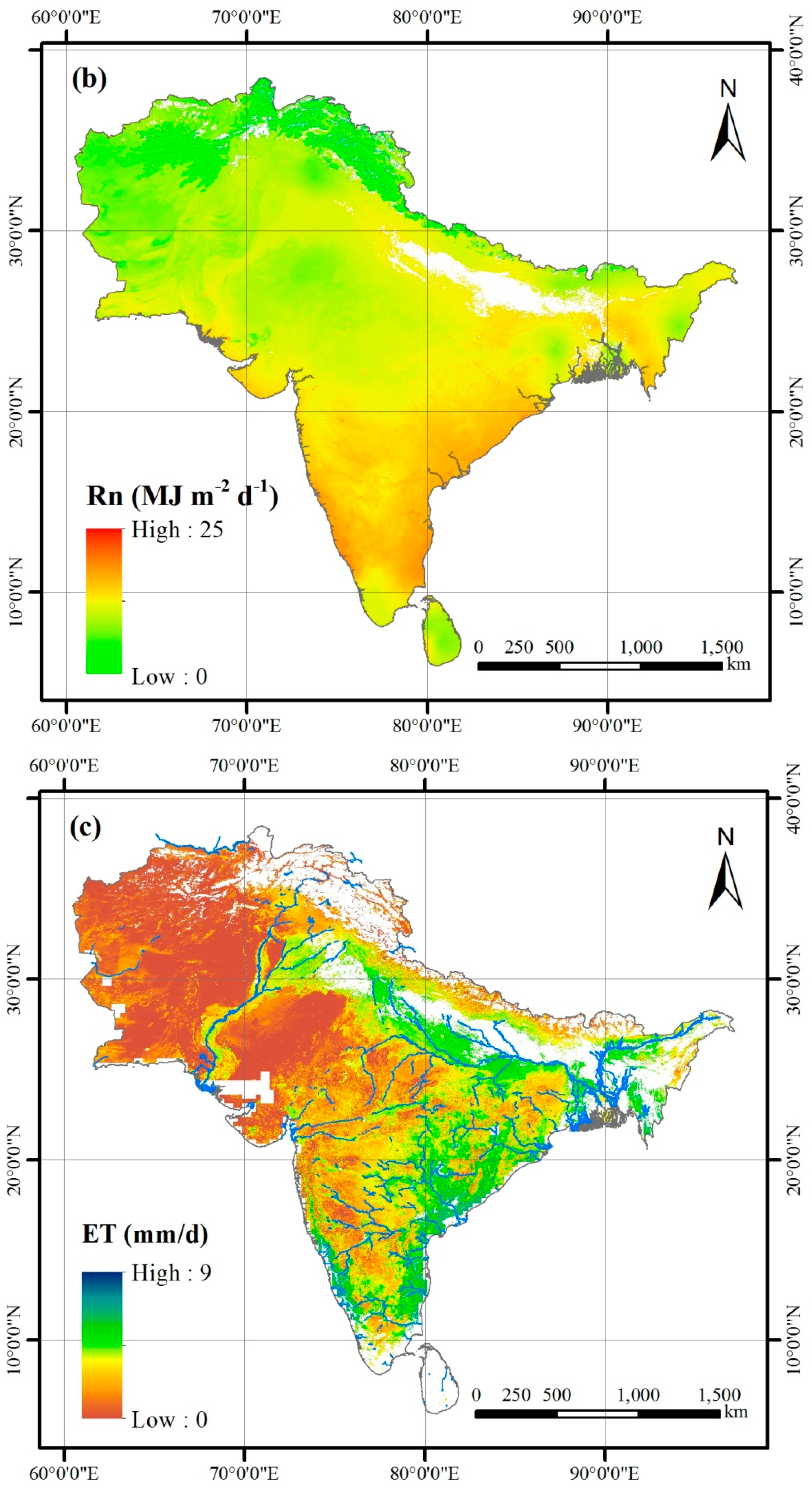
3.2.1. Daily Net Radiation

In Equation (8), the daily net radiation is composed by the net shortwave radiation (Rns) and net longwave radiation (Rnl). Numerous methods have been developed for the daily net radiation parameterization [36,37,38,39,40,41,42], and the methods generally differ in the complexity of their calibration structure and in their use of climatic parameters, variables, and coefficients. The developed and tested robust set of equations proposed by ASCE Environmental and Water Resources Institute (ASCE-EWRI) is suggested as the standardized procedures to calculate daily net radiation [43]. The comparison study suggested that the ASCE-EWRI estimated Rnd values had one of the best agreements with the measured daily net radiation (R2 = 0.93, RMSD = 1.44 MJ·m−2·d−1) [44]. Therefore, the ASCE-EWRI Rnd calculation procedures were used in the daily net radiation estimation.
The Rns is a result of the balance between incoming and reflected solar radiation. It can be expressed as:
R n s = ( 1 α ) R s
where α is surface albedo and Rs is total incoming shortwave solar radiation (MJ∙m−2∙d−1). Rs can be calculated using Angström’s formula, as recommended by Doorenbos and Pruitt [45]:
R s = ( 0.25 + 0.5 n N ) R a
where n/N is the ratio of actual measured bright sunshine hours and maximum possible sunshine hours, and Ra is extraterrestrial radiation expressed as the function of day of year, solar constant, declination and latitude (MJ·m−2·d−1):
R a = 1440 π G s c d r [ ω s sin ( φ ) sin ( δ ) + cos ( φ ) cos ( δ ) sin ( ω s ) ]
where Gsc is solar constant (0.0820 MJ ∙m−2∙ min−1), dr is inverse relative distance from earth to sun, ωs is sunset hour angle (rad), φ is latitude (rad), and δ is solar declination (rad).
For net longwave radiation, it is proportional to the fourth power of the absolute temperature of the surface[46,47]:
R n l = σ [ T max , K 4 + T min , K 4 2 ] ( 0.34 0.14 e a ) ( 1.35 R s R s o 0.35 )
where σ is Stefan−Boltzmann constant (4.903 × 10⁻⁹ MJ·K−4·m−2·d−1), Tmax,k is the daily maximum absolute air temperature (K), Tmin,k is the daily minimum absolute air temperature (K), ea is the actual vapor pressure of the air (kPa), and Rso is the calculated clear-sky solar radiation (MJ·m−2·d−1). The actual vapor pressure is estimated by:
e a = 0.6108 exp [ 17.27 T d e w T d e w + 237.3 ]
where Tdew is the dew point temperature (°C).
According to the formulas, several key atmospheric parameters (n, Tmax,k, Tmin,k, and Tdew) should be provided in order to calculate daily net radiation, and these parameters can be acquired from the records of the meteorological station observations. Therefore, the spatial interpolation method was applied to these parameters to get their spatial distribution in South Asia. A local Ordinary Kriging method was used to get the pixel value of each parameter from the nearby meteorological stations. Similar as the air temperature recalibration procedure, to account for the impact from altitude on Tmax,k, Tmin,k, and Tdew, a multiple variable linear fit was performed first for each parameter against latitude, longitude, and altitude. Then, the temperatures were normalized to the same altitude level according to the fitting coefficient of the altitude term. The normalized values were used finally to interpolate the pixel value and rescale to the pixel altitude level based on the coefficients. After the preparation of spatial distribution of the atmospheric parameters, the regional map Rnd of South Asia was achieved for each day.

3.2.2. Gap Filling and Daily, Monthly and Yearly ET Estimation

It is easy to derive daily ET when daily EF and Rnd are provided according to Equation (8). However, due to the blank values of an EF map due to cloud cover and scan gap, the estimated daily ET is likely to have many blank value areas. To avoid the impacts, a gap filling technique was applied to the estimated EF maps. For each pixel, usually there were some cloud cover days in each month, and their EF values are not available from the estimation. The common way to get the ET value of the cloud cover days is to fill it with the average value of the estimated ET pixel in one month [48]. However, the surface net radiation under cloud cover conditions is definitely different from the clear sky conditions, and the cloud cover reduces surface heating and evapotranspiration. Therefore, this approximation will bring big uncertainty to the ET estimation on cloud cover days. To avoid this problem, the ET estimation of the cloud cover days is performed by assuming that the average EF of the cloud-free days in one month can be used to represent the mean daily EF of this month, and approximate the EF value at the cloud cover or scan gap day. During this process, one thing should be considered: there may be few available EF values in one month, and the average value from the available EF values may have low temporal representativeness to represent the land surface evaporative conditions for other days with gap or cloud cover. Therefore, a constraint condition is set in the gap filling process that the number of available EF values of each pixel for each month should be no less than five (about one per week).
For monthly and yearly ET estimation, they are based on the daily ET estimation results. The simple integrating method is applied in both estimations. However, similar as daily ET estimation, the monthly average daily ET was firstly calculated with the available daily ET of each pixel for each month, and the monthly ET can be obtained based on average daily ET by multiplying the number of days in a month. The average monthly ET is then used to calculated yearly ET by multiplying the number of months in a year.

3.3. Validation Scheme

Quantitative validation is an important part of evaluating the accuracy of the ET estimations. Because there are few field ET observations available in South Asia, site by site evaluation is not suitable for this region. Therefore, cross-validation is the optimal way to quantify the accuracy of the ET estimation results. As introduced in the data sources section, the estimated monthly ET data was directly compared with the monthly ET from the GLDAS Noah monthly product at 0.25 degrees spatial resolution. In the GLDAS Noah monthly ET product, it contains straight averages of 3-hourly data, so that each monthly average has units: per 3 hours. The total ET parameter is the average 3-hour mean rate of evapotranspiration over all the 3-hour intervals for each month, and the monthly ET can be calculated by the average ET rate by multiplying the total seconds in each month. Taking April as an example, the total ET in this month (total_evapt(April)) is computed using this formula:
total _ evapt(April)  =  evapsfc(April) × 1 0 8 00 {sec/3hr} × 8{3hr/day} × 30 { days }
where evapsfc(April) is the average 3-hour mean rate of evapotranspiration over all the 3-hour intervals in April.
Because of the spatial differences between two datasets, the estimated monthly ET with fine resolution (1 km) should be aggregated into the coarse resolution (0.25 degrees) of GLDAS monthly ET product for cross-validation. Due to the existence of blank values in the estimated monthly ET, the aggregation should obey the rule that the available MODIS pixels of the estimated monthly ET data within the GLDAS product pixel size should occupy more than 90%, then the average value of the available pixels is used to approximate the monthly ET value at GLDAS product pixel scale.

4. Results and Validation

4.1. Daily and Monthly ET Estimation Result

Based on the daily ET estimation procedure provided in Section 3.2, daily ET of South Asia was retrieved for all days in 2008. Figure 3a presents the estimated EF on 2 March 2008 as an example. The spatial distribution of EF over the continent partly agrees with the surface water conditions in South Asia. The Indo-Gangetic Plain generally has relatively high EF due to the sufficient water supply. The Deccan Plateau in the middle and the northwestern semi-arid areas have smaller EF because of the limitations of wet and dry conditions. The blank area corresponds to cloud cover area and satellite scan gap due to the low latitude of South Asia. Figure 3b shows the estimated daily net radiation in South Asia ranging from 0 to more than 25 MJ∙m−2∙d−1. The overall spatial pattern of Rnd partly certifies its reasonability by the decreasing trend with the increase of latitude. In addition to the latitude influence, the surface conditions are also an important factor because of the differences in land surface water conditions and vegetation cover. As shown in the figure, the desert area in the northwest has relatively lower net radiation than that of the river plain due to the high albedo and emission. Similar results can be found from the net radiation study in Ma [49]. A blank area also exists in the Rnd map because of the null value in the MODIS albedo product.
Based on the gap filling method, the blank areas are avoided as much as possible in the estimated daily ET (Figure 3c). The spatial distribution of the estimated ET is consistent with the land surface wetness conditions over the whole region that the daily ET of the Indo-Gangetic Plain is significantly higher (more than 4 mm/d) than that of the northwestern desert and semi-arid areas (close to 0 mm/day) and the Deccan Plateau (lower than 4 mm/day). It is certain that the estimated daily ET map is more capable of representing the spatial variation of ET in South Asia after the gap filling process.
Based on the daily ET estimation results, the monthly ET of each month in 2008 in South Asia is derived with the method introduced in Section 3.2.2. Figure 4 is a color map of the monthly ET with the same color scale of 0–250 mm/month. It can be concluded that there are many blank areas in the map especially for months from June to September. Cloud cover is the first and the primary reason. In addition, the blank value of the MODIS albedo product in daily ET estimation is also another impact factor. Generally, from the visual inspection, the temporal change of monthly ET is able to indicate the common annual cycle of surface evapotranspiration with high ET in the middle year and low ET in the beginning and the end of the year.
Figure 3. (a) Evaporative Fraction (EF); (b) Daily net radiation and (c) Daily ET estimation results of South Asia on 2 March 2008.
Remotesensing 07 04726 g003aRemotesensing 07 04726 g003b
Figure 4. Monthly ET estimation results in South Asia in 2008.
Remotesensing 07 04726 g004

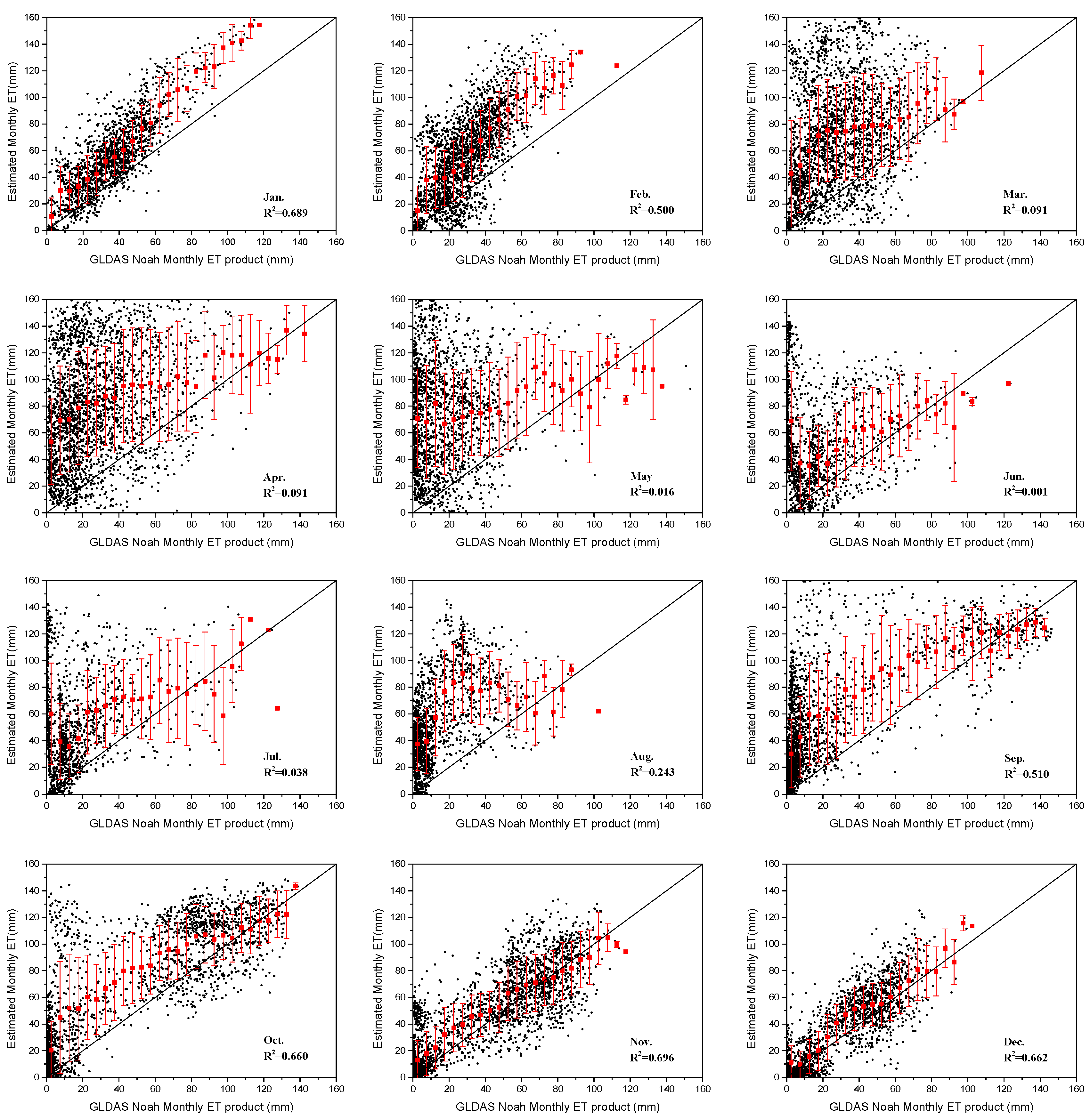
4.2. Validation and Analysis

With the monthly ET derived above, cross-validation was performed with the GLDAS monthly ET product. Figure 5 presents the comparison results between the estimated monthly ET and GLDAS monthly ET product according to the validation scheme shown in Section 3.3. From the scatter plot, it is clear that there is good correlation for the winter season (January, February, October, November, and December) with the R2 of 0.689, 0.500, 0.660, 0.696, and 0.662, respectively. However, obvious overestimation can be observed for the scatter plot in January, February, September and October. For the dry season (March to May), because the monthly ET estimates are considerably overestimated compared with GLDAS monthly ET, the R2 between two datasets in these months keep to a very low level. For the monsoon season (June to September), the estimated monthly ET in South Asia is largely filled by the blank values because of the heavy cloud cover in this season. The only cloud-free areas in these month are the northwest part of South Asia. Considerable overestimations also appear for these months, thereby inducing the poor correlation between them. The statistic values of the estimated monthly ET located in the GLDAS Noah monthly ET section certify the above fact. A mean ET profile for estimated monthly ET is estimated for each GLDAS monthly ET bin (size is 5 mm) by calculating bin-averaged estimated monthly ET values and ±1 standard deviation (vertical bars) in each bin. The red point in the middle of each bar is the mean value. The winter months from November to February show good correlation with a small standard deviation for each ET section. However, for the other months, especially for March to August, the mean value points generally do not obey the 1:1 line, and the standard deviation always keeps to a high value. This fact illustrates that the estimated monthly ET has large uncertainty in these months.
Figure 5. Scatter plot between estimated monthly ET and the NOAH GLDAS monthly product in 2008.
Remotesensing 07 04726 g005
From the scatter plots in Figure 5, it becomes clear that the monthly ET estimation in this study is usually overestimated for areas with low ET values in the GLDAS product for the months between March and October. March and June are selected as an example to analyze the overestimation during these two periods (dry season: March to May, and monsoon season: June to October). The difference between these two datasets in March and June is shown in Figure 6.
Figure 6. Monthly ET difference between the estimation result and the GLDAS product in March and June 2008. (a) presents the estimated monthly ET, (b) presents the GLDAS monthly ET product, (c) shows their difference in March, and (d) shows the NDVI spatial distribution of day of year (DOY) 81, 2008. (e) presents the estimated monthly ET, (f) presents the GLDAS monthly ET product, (g) shows their difference in June, and (h) shows the NDVI spatial distribution of DOY 161, 2008.
Remotesensing 07 04726 g006
In March, the overestimation areas are mainly located in the Indo-Gangetic Plain. The significant influence of water supply on land surface evaporation and transpiration processes can be exactly shown in the estimated monthly ET with monthly ET in the Indo-Gangetic Plain of over 100 mm and monthly ET in the Deccan Plateau of over 30 mm. However, the GLDAS product cannot show the difference between these two places with significant soil water conditions, and the Indo-Gangetic Plain has ET values (below 30 mm per month) similar to the Deccan Plateau. That is why the GLDAS ET product keeps to a low value, and the estimated monthly ET is highly overestimated in March. Meanwhile, the MODIS NDVI product (see Figure 6d) of day of year (DOY) 81, 2008 indicates that the Indo-Gangetic Plain has obviously better vegetation cover conditions than the Deccan Plateau. The NDVI in the Indo-Gangetic Plain is more than 0.5 while the NDVI for the Deccan Plateau keeps to a low value around 0.25. The higher vegetation cover in the Indo-Gangetic Plain is reasonable to maintain a higher evaporative rate. Therefore, the Indo-Gangetic Plain should have higher ET compared with other areas. From this point, it can be thought that the estimated monthly ET is more capable of capturing the land surface ET variation under different water and vegetation conditions. The small spatial differences and low value level of the GLDAS ET product from March to May induces the comparison result that the estimated monthly ET is much larger than GLDAS product in this period.
In June, the arrival of the monsoon brings water vapor to the subcontinent. Heavy cloud covers most of South Asia, except for the northwestern area. It can be reflected by the monthly ET data of June to October in Figure 4. In the northwestern area, due to its semi-arid or arid climate and low vegetation cover level (most part is below 0.2, see Figure 6h), land surface ET in this area mostly comes from the evaporation from soil surface. Therefore, it should keep to a low value due to the water stress and be enlarged after few rainfall events. The GLDAS ET product correctly presents the circumstance of this area. However, the estimated monthly ET has very high values in the southern part of this region. The same high ET area is also shown in July, August, September, and October. That is why there is a big overestimation for the low GLDAS ET range in the comparison shown in the scatter plot (June to October). The reason should be partly attributed to the error from atmospheric parameters. The large cloud cover in these month induces relatively fewer field observation stations involved in the land surface temperature calibration, and results in the underestimation of the near surface air temperature which underestimates the sensible heat flux and in turn enlarges the EF and ET in this region.
According to the cross-validation results, it is clear that the uncertainties related to the estimated ET have many sources. The major source mainly comes from the simplified process in ET estimation procedures.
In ET estimation procedure, the influence from soil heat flux estimation in SEBS should be considered. As introduced in the methods section, a simple empirical method is used to retrieve soil heat flux with Equation (5), as in previous studies [22,48,50]. The method is based on the relationship between fraction of vegetation cover (FVC) and soil heat flux to specify the ratio of G to net radiation. However, many studies [51,52] have shown that the ratio is not constant in space or in time and is highly dependent on soil moisture, soil texture, and vegetation cover. Therefore, Equation (5) cannot exactly reflect the influence of soil moisture difference on soil heat flux. Tanguy, et al. [53] proposed a new parameterization scheme of soil heat flux by linking the ratio to EF with a linear equation according to site observation data. It presents a new direction to consider the soil moisture effect on G. However, due to the lack of field observation of surface energy flux in South Asia, it is hard to build a suitable and robust equation for the whole region with large variation in soil moisture and land cover conditions. Therefore, the use of Equation (7) in this study will bring uncertainty in EF estimation especially for sparse vegetation or bare surfaces where the soil moisture conditions have a big variation.
The assumptions predefined in the daily ET estimation that: (1) the 24 h soil heat flux is negligible; and (2) the daily EF value is thought be constant and equal to the instantaneous EF value. Cammalleri, et al. [54] systematically figured out the effect of these assumptions on estimating daily ET. The neglect of soil heat flux will highlight errors on daily ET by increasing the net radiation, especially for sparse vegetated areas. The amount of soil heat can be substantial due to the fraction of bare soil exposed to direct radiation. The hypothesis of daytime constancy of EF causes an underestimation of daytime average value. Although the combined effect of the two assumptions exhibits a compensation effect, the error related to neglecting G will bring a significant residual error to ET estimation.
The other factor should be partly attributed to the EF estimation for cloud cover days. Usually, land surface in clear sky days will have higher ET values that those of cloudy sky days and consequently higher EF However, in the gap filling part, the estimation of EF in cloud cover days is based on the average value of EF values retrieved from clear sky conditions in the same month. This process will highlight the EF value when compared with the real value under cloud cover conditions. Therefore, the ET estimation in cloud cover days should be overestimated reasonably with the EF derived at clear conditions.
Besides the influence from the ET estimation procedures, the accuracy of ET estimates in the GLDAS product should be one impact factor. The purpose of GLDAS is to ingest satellite- and ground-based observational data products, using advanced land surface modeling and data assimilation techniques, in order to generate optimal fields of land surface states and fluxes. However, the validation work of GLDAS indicates that underestimation existed in the GLDAS ET product [55,56]. Rodell, et al. [55] used GRACE satellite gravity observations to get regional ET based on terrestrial water budget, and validated modelled ET from ECMWF, GLDAS, and GDAS. The daily comparison results pointed out that the GLDAS ET product underestimated ET with a mean bias of −0.62 mm/day. Xue, et al. [56] evaluated GLDAS ET products by estimating ET using a water balance method in the upper Yellow and Yangtze Rivers, and found that GLDAS ET estimates greatly underestimated ET in the upper Yangtze with a bias of −120.9 mm/year. The underestimation of the GLDAS ET product enlarges the overestimation of the estimated ET in the cross-validation.

5. Spatio-Temporal Variation Analysis

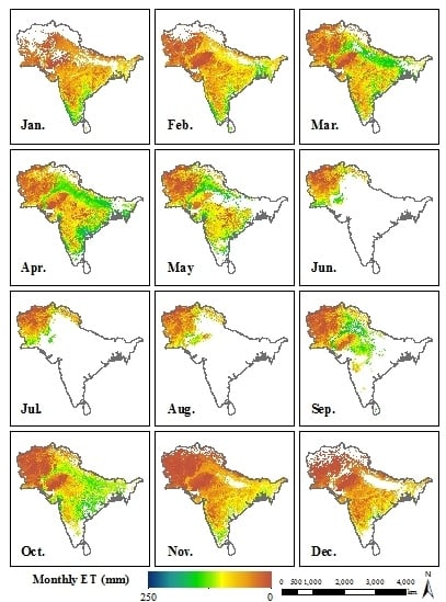
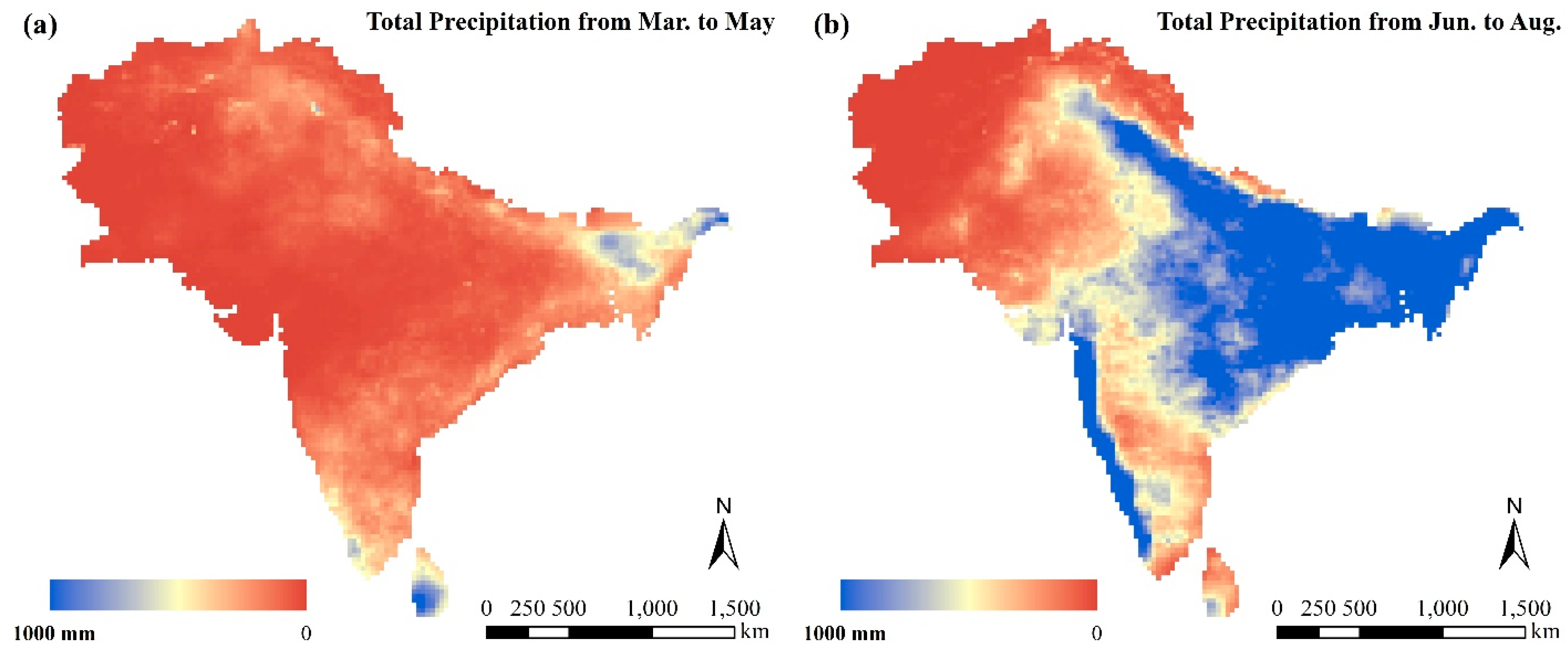
5.1. Monthly Variation

Regardless of the heavy cloud cover season (June to September), a simple spatio-temporal variation analysis was conducted for South Asia according to the monthly ET estimation results as shown in Figure 4. It is obvious that the change generally obeys the rule that the monthly ET increases from low value month (January and February) to high value month (March to October) and decreases to the low level again in November and December.
In January and February, due to relatively low temperature and minimum water flow of major rivers, most parts of South Asia have low ET except for the Ganges Delta and the southern area close to the coast with enough rainfall supplement and high temperature. The average monthly ET of the two months is around 50 mm and 80 mm, respectively. In spring and early summer (March to May), with the rise of river water flow and the planting of crops, the evaporation and transpiration effects were accelerated to have higher ET value in the Indo-Gangetic Plain than other areas. In the Deccan Plateau, the hot and dry weather conditions enable this region with the considerably lower ET. The precipitation data from Tropical Rainfall Measuring Mission (TRMM) estimation also confirms the characteristic. As shown in Figure 7a, the precipitation of pre-monsoon season (from March to May) is mainly located in the northern and eastern part of the Indo-Gangetic Plain and the southern area. For the central area (Deccan Plateau) and the northwestern area, less rainfall is observed in these regions. Because rainfall is an important source for land surface ET generation, the rainfall spatial distribution pattern agrees well with the spatial distribution pattern of ET in these three months.
During the monsoon season (June to August), the precipitation over the subcontinent has a great increase with the maximum of more than 2000 mm (see Figure 7b). The Deccan Plateau, the driest and hottest area in the dry season, also has plentiful rainfall (more than 500 mm) during this season. Only the northwestern area (Afghanistan and part of Pakistan) is cloud free. Therefore, the monthly ET of these months is only available in this region as shown in Figure 4. The cloud cover prevents the detection of the observation from satellite sensors. At the end of monsoon season, the sufficient precipitation has greatly improved the soil water conditions for most parts of South Asia. Therefore, the monthly ET of a large part of India has a high value in September and October. The increase of ET in the Deccan Plateau is most significant.
In November and December, with the kharif crops being harvested and the water flow declining in the Indus and Ganges Rivers, the monthly ET returns to the low value level (average value is around 50 mm per month) as that of January and February. In the annual cycle, when focusing on the northwestern area (Afghanistan and Pakistan), it is found that the monthly ET of this region always keeps to a low value, which is consistent with its semi-arid and arid climate conditions.
Figure 7. Total precipitation of (a) dry season (March to May) and (b) monsoon season (June to August) acquired from TRMM precipitation product.
Remotesensing 07 04726 g007

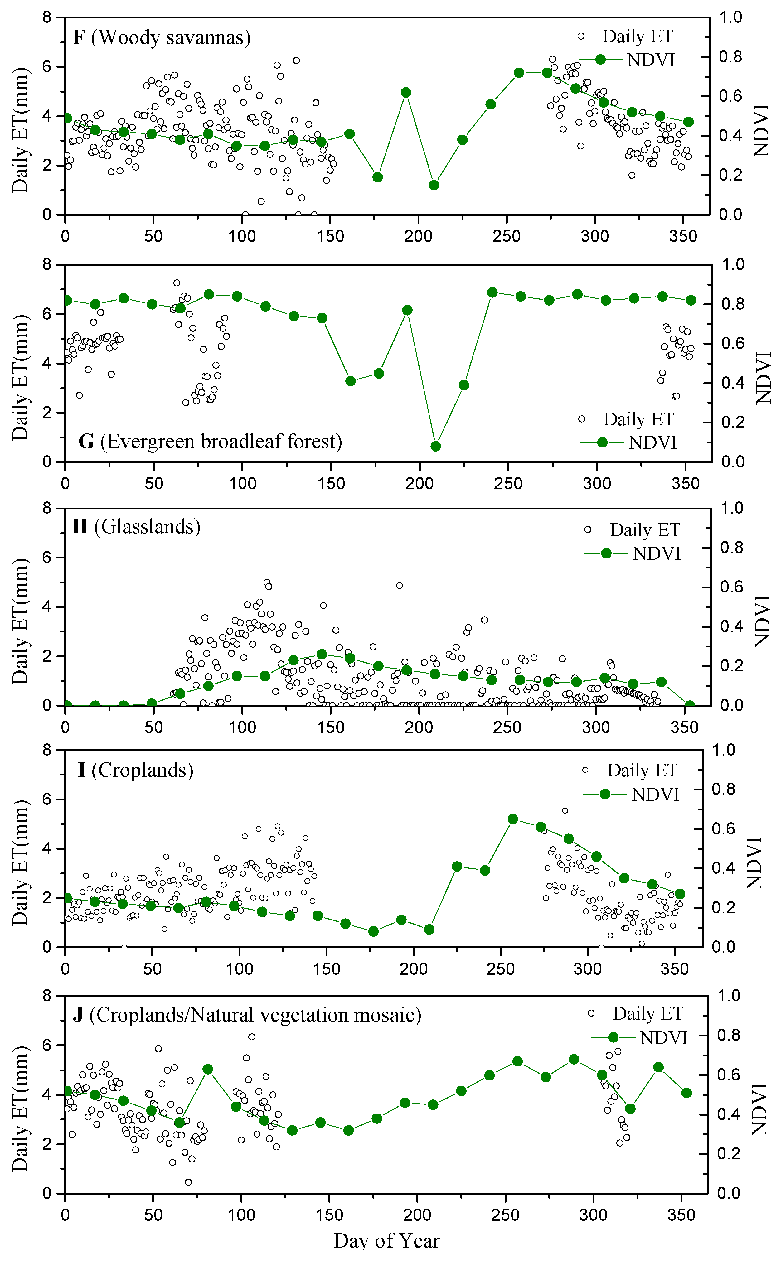
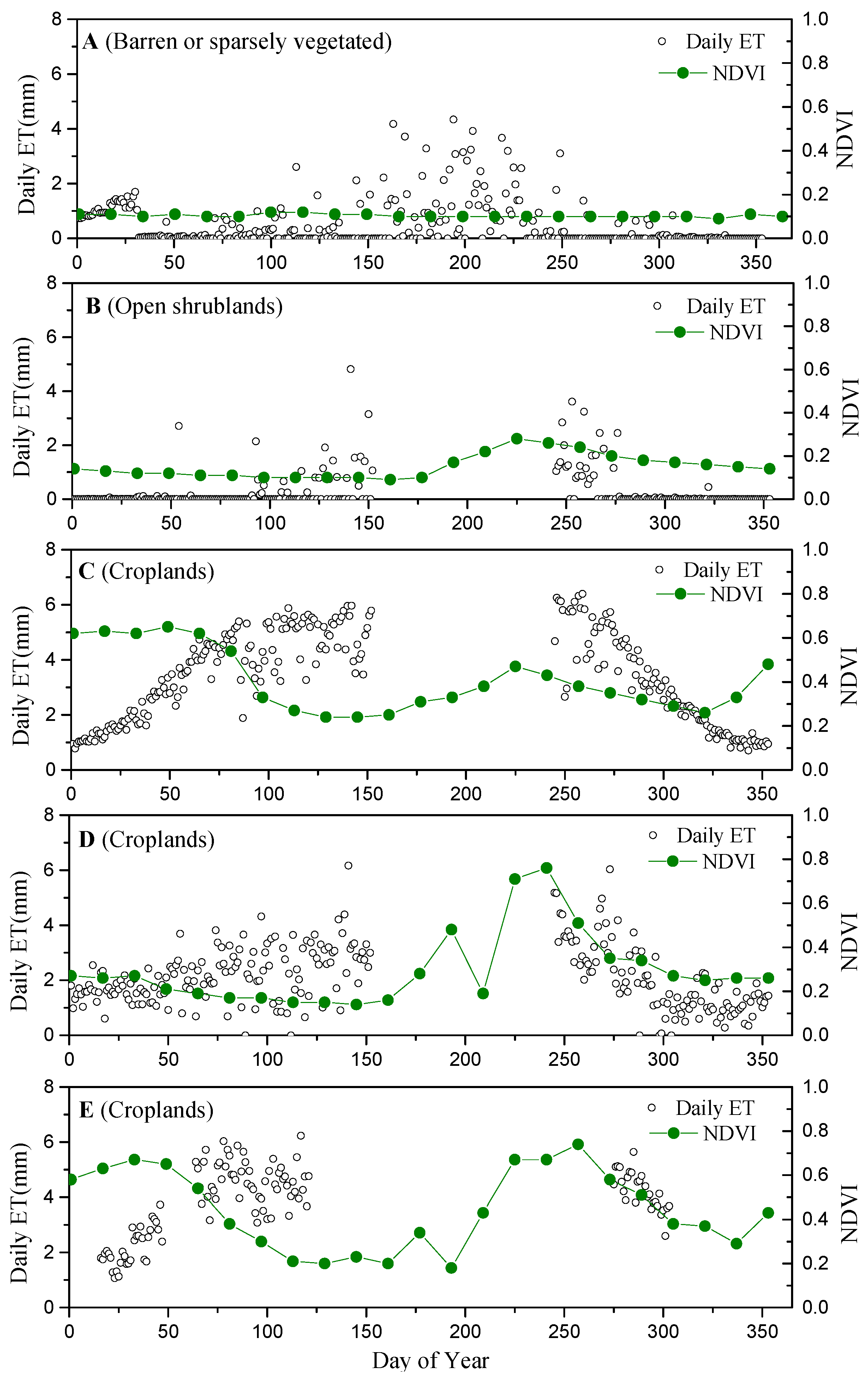
5.2. Typical Sites Analysis
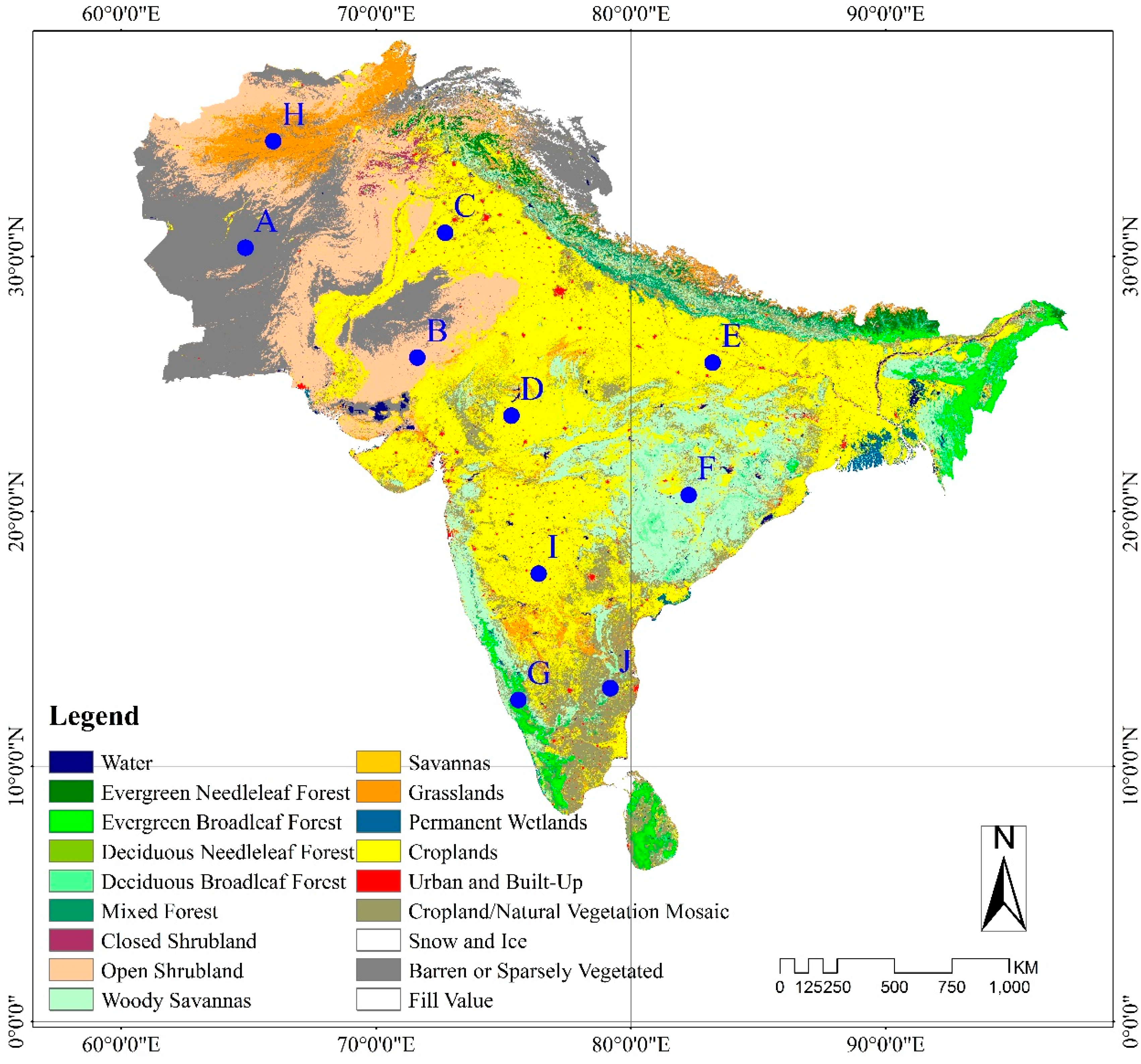
In addition to the regional analysis based on the monthly ET estimation results, a more detailed analysis is needed to analyze the spatial and temporal variation related to climate and vegetation cover. The land cover map was initially acquired from the MODIS land cover product (MCD12Q1) to understand the land cover conditions over the whole region. Figure 8 illustrates the International Geosphere-Biosphere Programme (IGBP) land cover map of the product in 2008. It is clear that a large part of South Asia is covered by cropland, including the Indo-Gangetic Plain and a large part of the Deccan Plateau. The areas in the northwest are chiefly covered by grassland and open shrublands, with barren or sparsely vegetated sections. The forests are mostly located along the mountain range in the north with parts in the south and east. In order to analyze the ET variation differences among different land cover types according to the land cover background, ten typical sites located at different climate environments with different land cover conditions were extracted to specify the spatio-temporal variation of ET in South Asia. The locations of the sites are plotted in Figure 8. Table 1 lists the geolocation, land cover type, country, and climate information of each site.
Figure 8. Land cover map of South Asia acquired from the MODIS land cover product and the locations of the selected ten sites.
Remotesensing 07 04726 g008
Table 1. Location and land cover information of sampling sites.
IDLatitudeLongitudeLand Cover TypeCountryClimate
A30.342664.8752Barren or sparsely vegetatedPakistanWarm desert
B26.032671.6239Open shrublandsIndiaWarm desert
C30.927972.7146CroplandsIndiaWarm semi-arid
D23.753575.313CroplandsIndiaTemperate continent
E25.828783.2057CroplandsIndiaHumid subtropical
F20.640882.2657Woody savannasIndiaTemperate continent
G12.606275.5879Evergreen Broadleaf forestIndiaTropical savanna
H34.519565.966GrasslandsAfghanistanCold desert
I17.554776.3772CroplandsIndiaWarm semi-arid
J13.067479.1973Cropland/Natural vegetation mosaicIndiaTemperate continent
The daily ET variation of the selected sites are depicted in Figure 9, with the temporal variation of NDVI at each site shown as the green line. In the site-by-site comparison, site A and B represent the typical desert or semi-arid and arid area in South Asia. It is clear that the average daily ET of point A and B keep to low values (0.5 mm and 0.3 mm, respectively) compared with other pixels because of the dry surface conditions. Another impact factor should be the low vegetation cover; it can be concluded from their NDVI values that the NDVI of both sites always keeps to a low value around 0.1. The surface ET mainly comes from soil evaporation. High daily ET only appears after some rainfall events during the monsoon season. Similar to the ET variation in sites A and B, the site H represents the major grassland in South Asia which is mainly located in Afghanistan. Its climate is cold desert. As shown in the plot, its daily ET also has a big annual variation. With the temperature rising in the spring and early summer, the winter snow melts and accelerates surface evaporation, which can be seen in the increase in daily ET. However, after late summer, its daily ET is always below 2 mm with the average of 0.8 mm. The low NDVI value also confirms the low ET value in this region.
Figure 9. Temporal variation of daily ET (cycle) and NDVI (green symbol line) of the sampling sites A-J with different land cover types listed in Table 1.
Remotesensing 07 04726 g009aRemotesensing 07 04726 g009b
For cropland regions, such as sites C, D, E, and I, they are located at different regions of South Asia, respectively representing different climate environments. Sites C and E are in the Indo-Gangetic Plain with a substantial water supplement from the Indus and Ganges Rivers. Sites D and I are located at the north and south of the Deccan Plateau. The temporal change of daily ET of these points generally has a similar trend in variation but also exhibits the differences in the ET magnitude due to the impact of water conditions. The daily ET of sites C and E increases from early spring and keeps to high values (more than 5 mm) during the summer and returns to low values in winter. They have similar NDVI temporal change patterns. The average daily ET of two pixels is of high value with 3.4 mm and 3.9 mm, respectively. The good surface water conditions in sites C and E is a key factor in enabling the surface evaporation and transpiration processes. While for sites D and I, because they are located in the Deccan Plateau, their ET effects are highly influenced by the rainfall event and their daily ETs have a systematic decrement with the average values of 2.1 mm and 2.2 mm, respectively. Their daily ETs have a gradually increasing trend during the year and drop quickly in winter with the NDVI decrement.
For the woody savannas of site F, the daily ET always keep to a relatively high level with average value of 3.4 mm, which can be reflected by the good vegetation cover conditions (NDVI more than 0.4) in this region. For sites G and J located in the south, it is reasonable that they both have a high ET level due to big energy availability and good surface water conditions with enough rainfall. The good vegetation cover is also one important factor for the high ET in sites G and J. In general, the temporal change pattern of daily ET for selected sampling pixels agree well with the monthly ET change pattern with the minimum value during the winter and the maximum value in the summer. Rainfall plays an important role on the spatial and temporal variation of ET in South Asia.

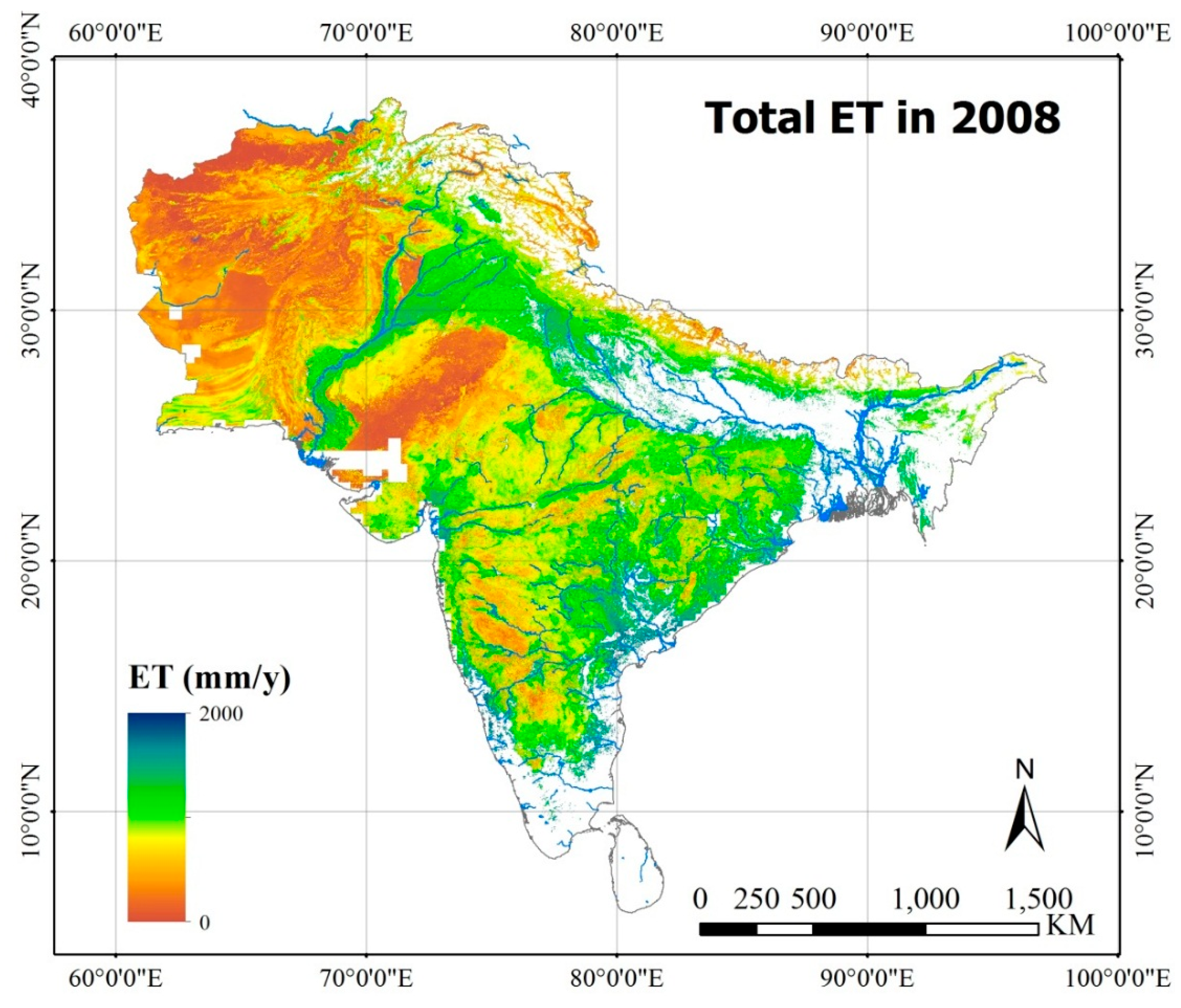
5.3. Annual Analysis

To better analyze the ET variation in South Asia, annual ET is derived based on the average monthly ET estimation by multiplying the number of months in a year. Figure 10 illustrates the total ET of South Asia in 2008. The ET spatial pattern generally reflects the impact from climate and vegetation distribution. The maximum annual ET places a major distribution at the Indo-Gangetic Plain and the river delta areas at the coast line with the value above 1000 mm/year. The northwestern area and the desert area around the boundary have the lowest annual ET because of the semi-arid or arid environment. The Deccan Plateau has the average annual ET of around 800 mm.
Figure 10. Annual ET spatial distribution in 2008 in South Asia.
Remotesensing 07 04726 g010
In addition to the annual ET spatial pattern analysis, the total ET in 2008 is plotted against the annual precipitation in 2008 (Figure 11). Good correlation is presented for two datasets with the linear fitted slope of 0.43. The R2 and the RMSD is 0.44 and 254.8 mm, respectively. It implies that precipitation is an important source to accelerate land surface ET, and its amount is bigger than the ET effect in many places of South Asia. However, in real situations, many places face more and more serious water scarcity with the appearance of severe drought disasters, especially in Pakistan and India. It can be explained by the unevenly distribution of precipitation during the year. Take India as an example: this region experiences a tropical monsoon climate, with significant seasonal variations in rainfall and temperature. About 80 percent of the total precipitation occurs during the monsoon period. Therefore, the understanding of ET spatial distribution in South Asia combined with precipitation data is very important for water resource management to deal with drought disasters in South Asia.
Figure 11. Scatter plot between annual precipitation and annual ET in South Asia in 2008.
Remotesensing 07 04726 g011

6. Conclusions

Accurate estimation of ET is essential for water resource management, especially for South Asia with its threat to water resources. In this study, time series of daily ET were estimated using the SEBS model for South Asia in 2008 based on Terra MODIS satellite products with other auxiliary atmospheric data from meteorological stations and the GLDAS product. Cross-validation work is performed by comparing the estimated monthly ET with monthly ET data from GLDAS ET product due to the lack of field ET observation data. Good agreements were found between two datasets in winter months with the R2 around 0.6. Although overestimation happens in the estimated monthly ET compared with GLDAS ET product, the spatio-temporal analysis implies the reasonability of the estimates of ET to be able to show the temporal change pattern and spatial differences over different regions.
The estimation results of the daily, monthly and annual ET in South Asia help us to understand the ET process in the water cycle of South Asia. It can be concluded that the surface ET in South Asia is significantly different than other places: the northwest and the desert areas have the lowest daily average ET (smaller than 1 mm); the Indo-Gangetic Plain has high daily ET because of the water supply from the Indus and Ganges rivers; the Deccan Plateau also suffers from water shortages due to the dry and hot conditions with the daily ET smaller than that of the Indo-Gangetic Plain. The pre-monsoon climate induces the dry and low daily ET in the Deccan Plateau, and the daily ET has a big improvement after monsoon. The monsoon climate dominates the ET variety for most parts of South Asia. The results can be helpful for regional water resources management, drought assessment, and agricultural and hydrological application in South Asia.
Generally, the estimation efforts conducted in this study illustrate that the retrieval method with the SEBS model can provide ET products at high spatio-temporal resolution and overcome the difficulty of less ground observations of surface energy fluxes in South Asia. However, the uncertainties associated with soil heat flux estimation, assumptions for daily ET estimation, and the approximation method used for the gap-filling process suggest that a further study should be performed to generate a more reliable ET in South Asia. Meanwhile, the monthly comparison result also demands a more systematic evaluation.

Acknowledgments

The authors would like to thank the anonymous reviewers for their useful comments and suggestions. The authors would also like to extend their thanks to National Climatic Data Center (NCDC) for providing ground-measured meteorological data. This work was jointly supported by Key Program (No.KZZD-EW-08-01) of the Chinese Academy of Sciences, the “Hundred Talents” Project, National natural science foundation project (No. 41271433 and No. 41401425), the External Cooperation Program of BIC of Chinese Academy of Sciences (GJHZ201320), and the West Light Foundation of Chinese Academy of Sciences.

Author Contributions

Ainong Li designed the framework of this research work, and finished the final version of this paper. Wei Zhao processed the major data sources including satellite data and field observation data, and drafted the preliminary version of this paper. Wei Deng assist the comparison and validation work for the estimation results.

Conflicts of Interest

The authors declare no conflict of interest

References

  1. Bastiaanssen, W.; Noordman, E.; Pelgrum, H.; Davids, G.; Thoreson, B.; Allen, R. SEBAL model with remotely sensed data to improve water-resources management under actual field conditions. J. Irrigat. Drain. Eng. 2005, 131, 85–93. [Google Scholar]
  2. Anderson, M.C.; Allen, R.G.; Morse, A.; Kustas, W.P. Use of Landsat thermal imagery in monitoring evapotranspiration and managing water resources. Remote Sens. Environ. 2012, 122, 50–65. [Google Scholar] [CrossRef]
  3. Biemans, H.; Speelman, L.H.; Ludwig, F.; Moors, E.J.; Wiltshire, A.J.; Kumar, P.; Gerten, D.; Kabat, P. Future water resources for food production in five South Asian river basins and potential for adaptation—A modeling study. Sci. Total Environ. 2013, 468–469, S117–S131. [Google Scholar] [CrossRef] [PubMed]
  4. Singh, D.; Tsiang, M.; Rajaratnam, B.; Diffenbaugh, N.S. Observed changes in extreme wet and dry spells during the South Asian summer monsoon season. Nat. Clim. Chang. 2014, 4, 456–461. [Google Scholar] [CrossRef]
  5. Mirza, M.M.Q. Climate change, flooding in South Asia and implications. Reg. Environ. Chang. 2011, 11, 95–107. [Google Scholar] [CrossRef]
  6. Auffhammer, M.; Ramanathan, V.; Vincent, J. Climate change, the monsoon, and rice yield in India. Clim. Chang. 2012, 111, 411–424. [Google Scholar] [CrossRef]
  7. Bandyopadhyay, A.; Bhadra, A.; Raghuwanshi, N.; Singh, R. Temporal trends in estimates of reference evapotranspiration over India. J. Hydrol. Eng. 2009, 14, 508–515. [Google Scholar] [CrossRef]
  8. Jhajharia, D.; Dinpashoh, Y.; Kahya, E.; Singh, V.P.; Fakheri-Fard, A. Trends in reference evapotranspiration in the humid region of northeast India. Hydrol. Process. 2012, 26, 421–435. [Google Scholar] [CrossRef]
  9. Mallick, K.; Bhattacharya, B.K.; Chaurasia, S.; Dutta, S.; Nigam, R.; Mukherjee, J.; Banerjee, S.; Kar, G.; Rao, V.U.M.; Gadgil, A.S.; Parihar, J.S. Evapotranspiration using MODIS data and limited ground observations over selected agroecosystems in India. Int. J. Remote Sens. 2007, 28, 2091–2110. [Google Scholar] [CrossRef]
  10. Li, Z.-L.; Tang, R.; Wan, Z.; Bi, Y.; Zhou, C.; Tang, B.; Yan, G.; Zhang, X. A review of current methodologies for regional evapotranspiration estimation from remotely sensed data. Sensors 2009, 9, 3801–3853. [Google Scholar] [CrossRef] [PubMed]
  11. Mu, Q.; Zhao, M.; Running, S.W. Improvements to a MODIS global terrestrial evapotranspiration algorithm. Remote Sens. Environ. 2011, 115, 1781–1800. [Google Scholar] [CrossRef]
  12. Gibson, L.A.; Jarmain, C.; Su, Z.; Eckardt, F.E. Estimating evapotranspiration using remote sensing and the Surface Energy Balance System—A South African perspective. Water SA 2013, 39, 477–483. [Google Scholar]
  13. Liu, Y.; Zhou, Y.; Ju, W.; Chen, J.; Wang, S.; He, H.; Wang, H.; Guan, D.; Zhao, F.; Li, Y.; Hao, Y. Changes of evapotranspiration and water yield in China’s terrestrial ecosystems during the period from 2000 to 2010. Hydrol. Earth Syst. Sci. Discuss. 2013, 10, 5397–5456. [Google Scholar] [CrossRef]
  14. Tang, R.; Li, Z.-L.; Tang, B. An application of the Ts-VI triangle method with enhanced edges determination for evapotranspiration estimation from MODIS data in arid and semi-arid regions: Implementation and validation. Remote Sens. Environ. 2010, 114, 540–551. [Google Scholar] [CrossRef]
  15. Tang, R.; Li, Z.-L.; Jia, Y.; Li, C.; Sun, X.; Kustas, W.P.; Anderson, M.C. An intercomparison of three remote sensing-based energy balance models using Large Aperture Scintillometer measurements over a wheat-corn production region. Remote Sens. Environ. 2011, 115, 3187–3202. [Google Scholar] [CrossRef]
  16. Bastiaanssen, W.G.M.; Menenti, M.; Feddes, R.A.; Holtslag, A.A.M. A remote sensing surface energy balance algorithm for land (SEBAL). 1. Formulation. J. Hydrol. 1998, 212–213, 198–212. [Google Scholar] [CrossRef]
  17. Roerink, G.J.; Su, Z.; Menenti, M. S-SEBI: A simple remote sensing algorithm to estimate the surface energy balance. Phys. Chem. Earth PT. B 2000, 25, 147–157. [Google Scholar] [CrossRef]
  18. Su, Z. The Surface Energy Balance System (SEBS) for estimation of turbulent heat fluxes. Hydrol. Earth Syst. Sci. 2002, 6, 85–100. [Google Scholar] [CrossRef]
  19. Allen, R.; Tasumi, M.; Morse, A.; Trezza, R.; Wright, J.; Bastiaanssen, W.; Kramber, W.; Lorite, I.; Robison, C. Satellite-based energy balance for Mapping Evapotranspiration with Internalized Calibration (METRIC)—Applications. J. Irrigat. Drain. Eng. 2007, 133, 395–406. [Google Scholar] [CrossRef]
  20. Gowda, P.H.; Howell, T.A.; Paul, G.; Colaizzi, P.D.; Marek, T.H.; Su, B.; Copeland, K.S. Deriving hourly evapotranspiration rates with SEBS: A lysimetric evaluation. Vadose Zone J. 2013, 12. [Google Scholar] [CrossRef]
  21. Ma, W.; Hafeez, M.; Ishikawa, H.; Ma, Y. Evaluation of SEBS for estimation of actual evapotranspiration using ASTER satellite data for irrigation areas of Australia. Theor. Appl. Climatol. 2013, 112, 609–616. [Google Scholar] [CrossRef]
  22. Timmermans, J.; Su, Z.; van der Tol, C.; Verhoef, A.; Verhoef, W. Quantifying the uncertainty in estimates of surface-atmosphere fluxes through joint evaluation of the SEBS and SCOPE models. Hydrol. Earth Syst. Sci. 2013, 17, 1561–1573. [Google Scholar] [CrossRef]
  23. Lu, J.; Li, Z.-L.; Tang, R.; Tang, B.-H.; Wu, H.; Yang, F.; Labed, J.; Zhou, G. Evaluating the SEBS-estimated evaporative fraction from MODIS data for a complex underlying surface. Hydrol. Process. 2013, 27, 3139–3149. [Google Scholar] [CrossRef]
  24. Su, H.; McCabe, M.F.; Wood, E.F.; Su, Z.; Prueger, J.H. Modeling evapotranspiration during SMACEX: Comparing two approaches for local- and regional-scale prediction. J. Hydrometeorol. 2005, 6, 910–922. [Google Scholar] [CrossRef]
  25. Ma, W.; Ma, Y.; Hu, Z.; Su, Z.; Wang, J.; Ishikawa, H. Estimating surface fluxes over middle and upper streams of the Heihe River Basin with ASTER imagery. Hydrol. Earth Syst. Sci. 2011, 15, 1403–1413. [Google Scholar] [CrossRef]
  26. Vinukollu, R.K.; Wood, E.F.; Ferguson, C.R.; Fisher, J.B. Global estimates of evapotranspiration for climate studies using multi-sensor remote sensing data: Evaluation of three process-based approaches. Remote Sens. Environ. 2011, 115, 801–823. [Google Scholar] [CrossRef]
  27. Gibson, L.A.; Münch, Z.; Engelbrecht, J. Particular uncertainties encountered in using a pre-packaged SEBS model to derive evapotranspiration in a heterogeneous study area in South Africa. Hydrol. Earth Syst. Sci. 2011, 15, 295–310. [Google Scholar] [CrossRef] [Green Version]
  28. Zhao, W.; Li, A.; Deng, W. Surface energy fluxes estimation over the South Asia subcontinent through assimilating MODIS/TERRA satellite data with in situ observations and GLDAS product by SEBS model. IEEE J. Sel. Top. Appl. Earth Obs. Remote Sens. 2014, 7, 3704–3712. [Google Scholar] [CrossRef]
  29. Kumar, S.V.; Peters-Lidard, C.D.; Tian, Y.; Houser, P.R.; Geiger, J.; Olden, S.; Lighty, L.; Eastman, J.L.; Doty, B.; Dirmeyer, P.; Adams, J.; Mitchell, K.; Wood, E.F.; Sheffield, J. Land information system: An interoperable framework for high resolution land surface modeling. Environ. Modell. Softw. 2006, 21, 1402–1415. [Google Scholar] [CrossRef]
  30. Rodell, M.; Houser, P.; Jambor, U.E.A.; Gottschalck, J.; Mitchell, K.; Meng, C.; Arsenault, K.; Cosgrove, B.; Radakovich, J.; Bosilovich, M. The global land data assimilation system. Bull. Am. Meteor. Soc. 2004, 85, 381–394. [Google Scholar] [CrossRef]
  31. Tang, B.; Li, Z.-L.; Zhang, R. A direct method for estimating net surface shortwave radiation from MODIS data. Remote Sens. Environ. 2006, 103, 115–126. [Google Scholar] [CrossRef]
  32. Tang, B.; Li, Z.-L. Estimation of instantaneous net surface longwave radiation from MODIS cloud-free data. Remote Sens. Environ. 2008, 112, 3482–3492. [Google Scholar] [CrossRef]
  33. Carlson, T.N.; Ripley, D.A. On the relation between NDVI, fractional vegetation cover, and leaf area index. Remote Sens. Environ. 1997, 62, 241–252. [Google Scholar] [CrossRef]
  34. Prihodko, L.; Goward, S.N. Estimation of air temperature from remotely sensed surface observations. Remote Sens. Environ. 1997, 60, 335–346. [Google Scholar] [CrossRef]
  35. Tang, R.; Li, Z.-L.; Sun, X. Temporal upscaling of instantaneous evapotranspiration: An intercomparison of four methods using eddy covariance measurements and MODIS data. Remote Sens. Environ. 2013, 138, 102–118. [Google Scholar] [CrossRef]
  36. Samani, Z.; Bawazir, A.S.; Bleiweiss, M.; Skaggs, R.; Tran, V.D. Estimating daily net radiation over vegetation canopy through remote sensing and climatic data. J. Irrigat. Drain. Eng. 2007, 133, 291–297. [Google Scholar] [CrossRef]
  37. Hurtado, E.; Sobrino, J. Daily net radiation estimated from air temperature and NOAA-AVHRR data: A case study for the Iberian Peninsula. Int. J. Remote Sens. 2001, 22, 1521–1533. [Google Scholar] [CrossRef]
  38. Hoyt, D.V. A model for the calculation of solar global insolation. Solar Energy 1978, 21, 27–35. [Google Scholar] [CrossRef]
  39. Konzelmann, T.; van de Wal, R.S.; Greuell, W.; Bintanja, R.; Henneken, E.A.; Abe-Ouchi, A. Parameterization of global and longwave incoming radiation for the Greenland Ice Sheet. Glob. Planet. Chang. 1994, 9, 143–164. [Google Scholar] [CrossRef]
  40. Kruk, N.S.; Vendrame, Í.F.; Da Rocha, H.R.; Chou, S.C.; Cabral, O. Downward longwave radiation estimates for clear and all-sky conditions in the Sertãozinho region of São Paulo, Brazil. Theor. Appl. Climatol. 2010, 99, 115–123. [Google Scholar] [CrossRef]
  41. Morcrette, J.-J.; Deschamps, P.-Y. Downward longwave radiation at the surface in clear-sky atmospheres: Comparisons of measured, satellite-derived, and calculated fluxes. In Proceedings of the International Satellite Land-Surface Climatology Project (ISLSCP) Conference, Rome, Italy, 2–6 December 1985.
  42. Prata, A. A new long-wave formula for estimating downward clear-sky radiation at the surface. Q. J. R. Meteorolog. Soc. 1996, 122, 1127–1151. [Google Scholar] [CrossRef]
  43. ASCE-EWRI. The ASCE Standardized Reference Evapotranspiration Equation: ASCE-EWRI Standardization of Reference Evapotranspiration Task Committe Report. Available online: http://www.irrisoft.net/downloads/literature/ASCE%20Standardized%20Equation%20Jan%202005%20Apendix%20A.pdf (accessed on 21 January 2015).
  44. Irmak, S.; Mutiibwa, D.; Payero, J.O. Net radiation dynamics: Performance of 20 daily net radiation models as related to model structure and intricacy in two climates. Trans. ASABE 2010, 53, 1059–1076. [Google Scholar] [CrossRef]
  45. Doorenbos, J.; Pruitt, W. Guidelines for predicting crop water requirements. In Irrigation and Drainage Paper; Food and Agriculture Organization of the United Nations: Rome, Italy, 1977. [Google Scholar]
  46. Brunt, D. Physical and Dynamical Meteorology; Cambridge University Press: Cambridge, UK, 2011. [Google Scholar]
  47. Brunt, D. Notes on radiation in the atmosphere. I. Q. J. R. Meteorolog. Soc. 1932, 58, 389–420. [Google Scholar] [CrossRef]
  48. Jin, X.; Guo, R.; Xia, W. Distribution of actual evapotranspiration over qaidam basin, an arid area in China. Remote Sens. 2013, 5, 6976–6996. [Google Scholar] [CrossRef]
  49. Ma, Y. Remote sensing parameterization of regional net radiation over heterogeneous land surface of Tibetan Plateau and arid area. Int. J. Remote Sens. 2003, 24, 3137–3148. [Google Scholar] [CrossRef]
  50. Ma, W.; Hafeez, M.; Rabbani, U.; Ishikawa, H.; Ma, Y. Retrieved actual ET using SEBS model from Landsat-5 TM data for irrigation area of Australia. Atmos. Environ. 2012, 59, 408–414. [Google Scholar] [CrossRef]
  51. Crawford, T.M.; Stensrud, D.J.; Carlson, T.N.; Capehart, W.J. Using a soil hydrology model to obtain regionally averaged soil moisture values. J. Hydrometeorol. 2000, 1, 353–363. [Google Scholar] [CrossRef]
  52. Mecikalski, J.R.; Diak, G.R.; Anderson, M.C.; Norman, J.M. Estimating fluxes on continental scales using remotely sensed data in an atmospheric-land exchange model. J. Appl. Meteorol. 1999, 38, 1352–1369. [Google Scholar] [CrossRef]
  53. Tanguy, M.; Baille, A.; Gonzalez-Real, M.M.; Lloyd, C.; Cappelaere, B.; Kergoat, L.; Cohard, J.M. A new parameterisation scheme of ground heat flux for land surface flux retrieval from remote sensing information. J. Hydrol. 2012, 454, 113–122. [Google Scholar] [CrossRef] [Green Version]
  54. Cammalleri, C.; Ciraolo, G.; La Loggia, G.; Maltese, A. Daily evapotranspiration assessment by means of residual surface energy balance modeling: A critical analysis under a wide range of water availability. J. Hydrol. 2012, 452–453, 119–129. [Google Scholar] [CrossRef]
  55. Rodell, M.; Famiglietti, J.S.; Chen, J.; Seneviratne, S.I.; Viterbo, P.; Holl, S.; Wilson, C.R. Basin scale estimates of evapotranspiration using GRACE and other observations. Geophys. Res. Lett. 2004, 31. [Google Scholar] [CrossRef]
  56. Xue, B.-L.; Wang, L.; Li, X.; Yang, K.; Chen, D.; Sun, L. Evaluation of evapotranspiration estimates for two river basins on the Tibetan Plateau by a water balance method. J. Hydrol. 2013, 492, 290–297. [Google Scholar] [CrossRef]

